Optimization and Engineering manuscript No.
(will be inserted by the editor)
Craig Bakker · Geo↵rey T. Parks
Received: date / Accepted: date
Abstract Riemannian Optimization (RO) generalizes standard optimization methods from Euclidean spaces to Riemannian manifolds. Multidisciplinary Design Optimization (MDO) problems exist on Riemannian manifolds, and with the di↵erential geometry framework which we have previously developed, we can now apply RO techniques to MDO. Here, we provide background theory and a literature review for RO and give the necessary formulae to implement the Steepest Descent Method (SDM), Newton’s Method (NM), and the Con-jugate Gradient Method (CGM), in Riemannian form, on MDO problems. We then compare the performance of the Riemannian and Euclidean SDM, NM, and CGM algorithms on several test problems (including a satellite design problem from the MDO literature); we use a calculated step size, line search, and geodesic search in our comparisons. With the framework’s induced met-ric, the RO algorithms are generally not as e↵ective as their Euclidean coun-terparts, and line search is consistently better than geodesic search. In our post-experimental analysis, we also show how the optimization trajectories for the Riemannian SDM and CGM relate to design coupling and thereby provide some explanation for the observed optimization behaviour. This work is only a first step in applying RO to MDO, however, and the use of quasi-Newton methods and di↵erent metrics should be explored in future research.
Keywords Multidisciplinary Design Optimization· Di↵erential Geometry· Riemannian Optimization
C. Bakker·G.T. Parks Department of Engineering University of Cambridge Cambridge, United Kingdom CB2 1PZ E-mail: [email protected]
Riemannian Optimization in Multidisciplinary
1 Introduction
There currently exist a variety of gradient-based optimization algorithms. These algorithms are well-understood and widely used, but most have been derived for flat spaces. However, it is possible to generalize these algorithms to curved spaces: Riemannian Optimization (RO) methods are gradient-based op-timization algorithms derived for Riemannian manifolds. Due to the increased mathematical technicality of these methods, and the fact that the traditional algorithms have proven to be as successful as they have, RO is not widely known or commonly used, but Multidisciplinary Design Optimization (MDO) may prove to be an ideal application opportunity.
MDO problems exist on curved spaces – the feasible design manifolds de-fined by the state equations (Bakker and Parks 2015a). Thus far, the literature only shows use of the traditional “flat” algorithms on MDO problems, but given that these curved spaces are, in fact, Riemannian manifolds, it makes sense to consider how RO algorithms might perform in an MDO context. With our di↵erential geometry framework, we can now do that. In this paper, we will consider some MDO problems and compare the Riemannian algorithms’ performance against that of the Euclidean algorithms. We intend to focus on convergence behaviour over computational cost (for the time being) in order to determine if further investigation into the use of these algorithms is warranted.
2 Background
2.1 Riemannian geometry
Here, we reiterate and summarize relevant portions of theory which we have previously presented in more detail (Bakker and Parks 2015a). Di↵erential ge-ometry is concerned with doing mathematics (such as calculus) on generally non-Euclidean spaces. In Euclidean geometry, the basic structures of space are linear: lines, planes, and their analogues in higher dimensions, but di↵ er-ential geometry deals with manifolds. Manifolds are abstract mathematical spaces which locally resemble the spaces described by Euclidean geometry but may have a more complicated global structure (Ivancevic and Ivancevic 2007); manifolds are like higher-dimensional versions of surfaces.
A Riemannian manifold is a di↵erentiable manifold with a symmetric, pos-itive definite bilinear form (known as the metric tensor). Given a Riemannian manifold M, the metric tensor gij defines an inner product, and this makes it possible to perform a number of di↵erent mathematical operations on the manifold. For example, the infinitesimal length on the manifold is
ds2=gijdwidwj (1)
where wi are the coordinates of the manifold. Note the use of index nota-tion with the summanota-tion convennota-tion here and in the rest of this paper unless otherwise indicated. Our index notation includes the use of superscripts and
subscripts to indicate contravariant and covariant indices, respectively. We recognize that using this convention can be disorienting from an engineering perspective, but this kind of notational bookkeeping is significant for calculat-ing derivatives and handlcalculat-ing coordinate system changes, among other thcalculat-ings, so we will hold to it as much as possible; we explain this further in our foun-dational theory paper (Bakker and Parks 2015a).
The summation convention is that repeated indices in an expression are summed over:
aibi=X
i
aibi (2)
If gij is known at a point onM, it is possible to calculate the Christo↵el symbols at that point:
i kl = 1 2g im ✓ @gmk @wl + @gml @wk @gkl @wm ◆ (3) and they feature in two important places: the covariant derivative and the geodesic equation; i
kl are essentially intermediate quantities – they are typ-ically used for calculating other pieces of information. The geodesic equation is
¨
wi+ kliw˙kw˙l= 0 (4)
Solutions of the geodesic equation are the paths that particles moving along the manifold would take if they were not subjected to any external forces (Ivancevic and Ivancevic 2007). They are to curved spaces what straight lines are to flat spaces: great circles on a sphere are a familiar example.
The covariant derivative, denoted with a subscript semi-colon, does two things: it projects the derivative onto the tangent space (Boothby 1986), and it maintains the tensorial character of whatever it derivates (Ivancevic and Ivancevic 2007). vi,j is the derivative of vi with respect to wj (w are still the manifold coordinates), andvi;j is then thecovariant derivative ofvi with respect towj. The some sample formulae for the covariant derivative are
v;ki =v,ki + jki vj (5)
vi;k=vi,k ikjvj (6)
tikl;q =tikl,q+ qsi tkls kqstisl lqstiks (7) Notice how covariant and contravariant indices are di↵erentiated di↵ er-ently; also,gij;k= 0 (Szekeres 2004).
2.2 MDO background
MDO deals with the optimization of systems which have coupled subsystems. The field originally grew out of structural optimization in aerospace design at NASA in the 1980s. Today, it is applied across a range of engineering disci-plines, but aerospace remains a significant application area. In MDO, prob-lem coupling is dealt with through decomposition and coordination strategies called architectures. Martins and Lambe (2013) provide a comprehensive re-view of MDO architectures and describe their functioning in detail.
A key part of performing optimization with these architectures is obtaining relevant derivative information. The Global Sensitivity Equations (GSEs) are a well-known way of obtaining the total derivatives of state variables with re-spect to design variables by using partial derivative information from each dis-cipline (Sobieszczanski-Sobieski 1990). Optimum Sensitivity Analysis (OSA) can be used similarly to obtain useful derivative information in multi-level op-timization problems, such as those which result from using MDO architectures (Barthelemy and Sobieszczanski-Sobieski 1983), and adjoint derivatives have also proved to be useful in computationally expensive MDO contexts (Mar-tins et al. 2005). Mar(Mar-tins and Hwang (2012) summarize most of the relevant information regarding derivative calculations in MDO.
MDO also has connections to a variety of related fields: optimal control (Allison and Herber 2013), multi-objective optimization (Tappeta et al. 2000), metamodelling (Paiva et al. 2010), and multi-fidelity modelling (Thokala 2005). These connections continue to be explored alongside research in basic MDO methods and MDO applications.
2.3 MDO in Riemannian geometry
In this section, we summarize the translation of MDO into Riemannian geom-etry (Bakker and Parks 2015a). Consider a generic MDO problem as
minf(x,y,z) (8)
g(x,y,z)0 (9)
h(x,y,z) =0 (10)
where x is the vector of local design variables, y is the vector of state vari-ables,z is the vector of global design variables, g is the vector of inequality constraints, andhis the vector of state equations in residual form; (10) is just a rearrangement of the state equations:
yi= i(x(i),˜y(i),z), i= 1,2, . . . (11) where x(i) is the set of local variables for discipline i and ˜y(i) is the set of all state variables excludingyi. A two-discipline example of this is shown in
Fig. 1 A Two-Discipline MDO Schematic
schematic form in Fig. 1. The variables can be further simplified by lumping them together:w={x z} andv={w y}.
The total design space for this problem is<m, wheremis the total number of variables, and the feasible design spaceMf easis ann-dimensional manifold, where n is the total number of design variables, defined by the solutions to the state equations; Mf eas is a subspace of the total design space. Assuming sufficient di↵erentiability, the induced metricgij onMf eas is
gij = @v k @wi @vk @wj = ij+ @yk @wi @yk @wj (12)
where the derivatives of y with respect to w are calculated from the state equations by using the implicit function theorem. The Christo↵el symbols are then i kl=gim @ys @wm @2ys @wk@wl (13)
Turning to the objective function derivatives, we know that for a scalar function, the covariant derivative is identical to the regular derivative:
f;i=f,i= df dwi = @f @wi + @f @yk @yk @wi (14)
This is just the reduced gradient off. However, taking the covariant deriva-tive again does not result in the reduced hessian. The reduced hessian and the second covariant derivative off are, respectively,
f,ij= @ 2f @wi@wj + @2f @wi@yk @yk @wj + @2f @wj@yk @yk @wi + @2f @ym@yk @yk @wi @ym @wj + @f @yk @2yk @wi@wj (15) f;ij =f,ij ijlf,l (16)
As we have noted previously (Bakker and Parks 2015a), this di↵erential geometry perspective allows us to consider the constrained optimization prob-lem as an unconstrained probprob-lem on a Riemannian manifold. The resulting Lagrangian (on the Riemannian manifold) could have inequality constraint terms, but it would not have equality terms corresponding to the state equa-tions because those constraints would have already been “absorbed”, for lack of a better term, into the Riemannian manifold and its structure; any additional non-state equality constraints could feature in the Lagrangian, though.
Since the variety of variables used in this paper could prove confusing, we have provided a list of commonly used terms, in both vector (boldface) and index notation where appropriate, in Table 1.
Table 1 Commonly Used Quantities
Symbol Denotation
f Objective function
g,gi Vector of inequality constraints h,hi Vector of state equations in residual form w,wi Vector of all design variables
x,xi Vector of all local design variables z,zi Vector of all global design variables
y,yi Vector of state variables (defined by the state equations) gij,g Metric tensor
i
jk Christo↵el symbols a;i Covariant derivative ofa ↵(k) Step length at iterationk d(k) Step direction at iterationk
2.4 Theoretical background for Riemannian optimization
The metric tensor can be used to raise and lower indices. Consider the inner product hu,vi. In general, this can be expressed as gijuivj; in flat spaces, wheregij = ij,
gijuivj = ijuivj=ujvj (17)
This procedure can actually be considered as simply taking the covariant form of u, uj = gijui, and doing a tensor contraction with v: ujvj. This is relevant because of how it relates to objective function derivatives and gradi-ents. Technically, the objective function derivative @@xfi =f,iis a covector, not
a vector. However, the gradient is a vector, so we use the metric tensor inverse to raise the necessary index and getgijf,j as our gradient.
Geodesics, which are defined by (4), are an integral part of most RO derivations and proofs. In<n, gradient-based optimization algorithms do line searches; in RO, the search is done along geodesics (at least in theory). A
geodesic extending in the direction⇠at pointxcan be denoted by expx(t⇠) :
TxM !M,t >0. The exponential maps vectors inTxM to the manifold itself
(Boothby 1986).
Although this notation is simple and elegant, in practice, these geodesics are difficult to calculate (Yang 2007) as they require the solution of the geodesic equation. Geodesics are often used in convergence proofs for RO algorithms (da Cruz Neto et al. 1998; Ferreira and Svaiter 2002; Luenberger 1972). In practical calculations, however, geodesics are usually approximated with a tangent step with a constraint restoration step or a quadratic approximation (Gabay 1982). Fortunately, it is still possible to do the convergence analysis with these approximations (Qi 2011).
In order to implement these more computationally tractable problems, we need retractions. Retractions are first-order approximations to the exponential: Rx:TxM !M (Qi et al. 2010). For a vector⇠at a pointx,
Rx(⇠) = expx(⇠) =x+⇠ (18)
Baker (2008) gives three conditions for a retraction: 1. R is continuously di↵erentiable
2. Rx(0x) =x(0x is the zero element on TxM)
3. DRx(0x) = 1TxM, the identity mapping on TxM
Another important concept is that of parallel or vector transport. Parallel transport is the transportation of vectors between tangent spaces which pre-serves vector lengths and angles (Ji 2007); it applies analogously to moving tensors between the products of tangent and cotangent spaces (Whiting 2011). There is a connection which “connects” those tangent spaces. The connection is like a di↵erential equation which specifies how quantities on the manifold change locally, and we can represent that connection with the Christo↵el sym-bols. Parallel transport is the integration of the connection along a path (Whit-ing 2011), and thus parallel transport is actually defined by the connection (Li and Wang 2008).
Furthermore, for a given metric, there is a unique metric-compatible, sym-metric connection (Boothby 1986). This connection may be easy to specify, but it is difficult to compute parallel transport in practice (Nishimori 2005). Therefore, Qi (2011) defines vector transport as a relaxation of parallel trans-port corresponding to retraction as a relaxation of the exponential mapping.
Finally, we consider convexity. In<n, convexity of both sets and functions is defined with respect to straight lines: a functionf is convex if
f(tx+ (1 t)y)tf(x) + (1 t)f(y), t2[0,1] (19) and a setS is convex if
tx+ (1 t)y2S 8x, y2S, t2[0,1] (20)
In Riemannian geometry, however, convexity is defined with geodesics in-stead of straight lines (Bento et al. 2012); assuming that there is a unique Riemannian Optimization in Multidisciplinary Design Optimization 7
geodesic (t) connectingxandy such that (0) =xand (1) =y, a function f is convex if
f( (t))tf(x) + (1 t)f(y), t2[0,1] (21) and a setS is convex if
(t)2S 8x, y2S, t2[0,1] (22)
When geodesic uniqueness fails, so too does a unique definition of convexity (Udri¸ste 1994). For a metric-compatible connection, convexity is in fact deter-mined by the choice of metric tensor (Rapcs´ak 1991): convexity is determined by the geodesics, which are determined by the connection, which is in turn determined by the metric tensor. Convexity is not, however, determined by the coordinate system used (Udri¸ste 1996a). This means that it is sometimes possible to transform nonconvex problems into convex problems through the choice of a favourable metric tensor (Bento et al. 2012).
2.5 A review of the field
Luenberger (1972) wrote the first significant paper applying RO to equality-constrained optimization. He used a projection operator to get the objective function derivatives onto the tangent spaces (using the coordinates of the em-bedding space, not coordinates specifically for the manifold itself) and proved convergence for a descent method along the manifold geodesics.
What may perhaps be considered the foundational paper, however, was later written by Gabay (1982). Gabay began from a constrained optimization problem and used slack variables to convert the inequality constraints into equality constraints. This is a fairly common practice in RO (Rapcs´ak 1989; Tanabe 1982). He then addressed the question of partitioning the problem into dependent and independent variables. Although some problems may have a natural partition available to them, arbitrary partitions may lead to poor performance. Throughout the rest of the paper, though, he avoided partitions and used projections from the embedding spaces instead of an explicit mani-fold coordinate representation. This is also fairly common when applying RO to general nonlinear optimization problems (Luenberger 1972; Rapcs´ak and Thang 1995; Tanabe 1980). Rheinboldt (1996) is a notable exception in us-ing a QR factorization on the constraint derivatives to get an orthonormal coordinate system at any given point on the manifold. Finally, considering two di↵erent types of geodesic approximation (a tangent step with constraint restoration and a quadratic approximation), Gabay (1982) developed a Rie-mannian version of a quasi-Newton method.
Since then, several authors have developed Riemannian versions of algo-rithms such as the Steepest Descent Method (SDM), Newton’s Method (NM) and the Conjugate Gradient Method (CGM) (Smith 1994; Udri¸ste 1994). How-ever, implementing geodesic searches is difficult to do in general. As a result,
many of the examples given to demonstrate the algorithms use special mani-folds – the Grassman and Stiefel matrix manimani-folds are particularly popular – where it is relatively easy to calculate the requisite quantities (Nishimori 2005; Qi 2011; Rapcs´ak 2002; Smith 1994).
In order to address this better, Qi (2011) looked in more detail at how to approximate the geodesic search typically specified by the RO algorithms proposed. She showed that the exponential map could be relaxed to the more general retraction while maintaining algorithm convergence and gave condi-tions and proofs for that convergence. Furthermore, di↵erent retractions ac-tually produce di↵erent optimization algorithms. As Ring and Wirth (2012) later pointed out, some retractions are better than others: there is a problem-specific tradeo↵between computability and the number of iterations required for convergence.
Baker (2008) continued to look at retraction-based RO while extending trust region methods to RO. Instead of directly applying Euclidean optimiza-tion algorithms to Riemannian manifolds, he used the retracoptimiza-tion to lift the objective function on the manifold to the manifold tangent spaces and then applied the Euclidean algorithms on those flat spaces. For example, he would use one retraction to build a trust region model in a tangent space, but he showed that a di↵erent retraction could then be used to explore that trust region model. He further showed that this process, even using two di↵erent retractions, was still convergent.
As already noted, the majority of the RO studies focused on equality-constrained optimization; slack variables would be used to turn any inequal-ities into equalinequal-ities. There were, however, some exceptions to that general methodology. Udri¸ste (1996b) used a logarthmic barrier function, and Ji (2007) explored this in more detail. Ji focused on interior-point methods and self-concordant functions, and he developed damped versions of SDM, NM, and CGM to deal with these inequality-constrained RO problems. Udri¸ste (1994) also considered using a method of feasible directions to address the same issue. In parallel to all of this, Tanabe (1979a; 1979b; 1980; 1982) looked at con-tinuous analogues to these discrete optimization processes in a Riemannian context. Typically working through the projection-based approach of Luen-berger and Gabay, Tanabe used continuous versions of descent and constraint satisfaction processes (with components tangent and normal to the manifold, respectively) to define the optimization problem. He then used di↵erential ge-ometry to analyze those dynamical systems on the manifold; the constrained optimization could be solved with a numerical Ordinary Di↵erential Equation (ODE) integrator. Dean (1988) later continued on in this vein and claimed that the problems thus generated were easier to analyze than the correspond-ing discrete optimization algorithms.
Alongside algorithm development, there have also been a variety of perti-nent theoretical works done on the subject. Yang (2007) and Qi (2010) sep-arately worked to generalize the Euclidean Armijo search conditions to RO. Ferreira and Svaiter (2002) similarly extended Kantorovich’s theorem to NM on Riemannian manifolds. A number of proofs for the convergence of geodesic-Riemannian Optimization in Multidisciplinary Design Optimization 9
based descent methods were produced (e.g. (da Cruz Neto et al. 1998)), but most of these proofs required certain curvature conditions on the manifold. Wang (2011), however, provided a curvature-independent convergence proof.
On a more applied level, some authors had interesting experiences with choosing di↵erent metric tensors. Udri¸ste (Udri¸ste 1996b), for example, pro-posed using the hessian of the Lagrangian (for an inequality-constrained RO problem) as a metric tensor; this could work to enforce feasibility during the optimization process. The nature of manifolds with objective function hes-sians as their metric tensors was, however, still an open problem 20 years ago (Udri¸ste 1994); any current advancements in this regard are unknown to us. In general, though, it is possible to choose the metric tensor in order to take advantage of problem-specific behaviour if enough is known about the problem beforehand, and doing this does not a↵ect the location of the optima (Ring and Wirth 2012). Munier (2007) provided an example of this: by choosing a particular metric tensor and using RO on the Rosenbrock problem, he was able to turn the problem into a convex optimization, and this produced a far more efficient solution process than the typical Euclidean methods.
There are three other areas worth mentioning, though we will not go into them in detail. Firstly, Bento et al. (2012) touched on Multi-Objective Opti-mization (MOO) on Riemannian manifolds in their paper. We have not seen any other work in this area, but given that single-objective RO is as estab-lished (though small) as it is, it makes sense to expand into multiple objectives. Secondly, Whiting (2011) looked at path optimization on Riemannian mani-folds. This ties in to the calculus of variations and ultimately control problems in Riemannian geometry. Although we have not closely investigated this, we suspect that there exist a number of other works considering Riemannian con-trol problems. Thirdly, Potra and Rheinboldt (1989) considered a di↵erential geometric approach to Di↵erential Algebraic Equations (DAEs). DAEs are related to equality-constrained optimization through constrained ODE-based optimization (Tanabe 1980). Given the presence of di↵erential constraints in control problems, the study of these systems is probably also relevant to con-strained optimal control problems.
2.6 Comments on Riemannian optimization
A variety of theoretical results and methods has been produced for RO. Es-sentially, if it can be done in <n, it can be done analogously in Riemannian geometry (e.g. trust region methods, quasi-Newton methods), and there are a plethora of accompanying convergence proofs; this likely reflects the fact that most of the RO researchers are mathematicians, not engineers.
One of the difficulties in applying these methods to real optimization prob-lems is finding appropriate manifold coordinate systems. Applications of the methods tend to fall into one of two groups: using projections with matrix no-tation to stay in the coordinate system of the embedding space (Gabay 1982; Luenberger 1972; Tanabe 1980), or working on manifolds with a special
ana-lytical structure that permits the explicit calculation of the relevant quantities (Nishimori 2005; Qi 2011; Rapcs´ak 2002; Smith 1994). The former perspective is general but fails to take advantage of the techniques and tools available for dealing with explicit manifold coordinates, and the latter approach is useful in specific contexts but only deals with a small subset of constrained nonlinear optimization problems. Essentially, coordinates (of some sort) are needed to do the calculations, and, in general, the mathematics are more easily grasped in a coordinate-based tensor notation than in either matrix or coordinate-free notation.
3 Applying Riemannian optimization to MDO
With our di↵erential geometry framework, we can now apply RO algorithms to MDO; we have an explicit coordinate representation, and we can calculate all of the relevant quantities. Furthermore, although we will not do this here, we could use our previous derivations (Bakker et al. 2012) and apply these Riemannian algorithms to several di↵erent MDO architectures.
In this paper, we will only consider gradient-based optimization techniques (SDM, NM, and CGM), not metaheuristic methods. The key di↵erences be-tween Riemannian and Euclidean optimization techniques lie in how deriva-tive information is handled and the path along which searching is done once a search direction has been chosen; the former, at least, would not apply to 0-th order methods. Given that metaheuristics are often designed to avoid the need for gradient information – a metaheuristic method might be chosen because the objective function is not smooth – this takes away a significant amount of potential overlap between metaheuristics and RO. For a method like Particle Swarm Optimization (Kennedy and Eberhart 1995), for example, there might still be the possibility of having the particles move along geodesics instead of straight lines, but calculating the geodesics would require second-order derivative information about the state equations, so RO methods may not be very helpful here, either. Although there may be potential crossover between metaheuristics and RO, we will not explore that here.
3.1 Algorithm formulae
Consider a general optimization algorithm to be
w(k+1)=w(k)+↵(k)d(k) (23)
where k in brackets indicates the iteration,w are the design variables, d is the step direction, and ↵ is the step length. To derive SDM and NM, let us start with a second-order Riemannian Taylor series about (with no loss in generality) the origin:
f wi =f(0) +f,iwi+1 2f;ijw
iwj (24)
As we have already noted, the gradient is not f,i but gijf,i and thus our descent direction for SDM isdi= gijf,j. If we wish to explicitly calculate a step length↵, we substitutewi=↵diinto (24), di↵erentiate, solve for↵, and get
↵= g
ijf,if,j
gijf,jf;ikgklf,l (25)
For NM, we start from (24) and di↵erentiate to find an optimal search directiondj and step length all at once. We get
f;ijdj = f,i (26)
If we let ⌘ij= [f;ij] 1
, thendj = ⌘ijf,i; it is implied that↵= 1 for NM. For CGM, we will not rederive the method from scratch, but we will give the formulae for Riemannian CGM (using a Fletcher-Reeves update scheme for the step direction). For CGM, the first step and any restart step is the same as that of SDM. After that,
↵(k)= ✓ dif,i dif;ijdj ◆ (k) (27) di (k)= gijf,j (k)+ f,igijf,j (k) (f,igijf,j) (k 1) di (k 1) (28)
The subscript index in parentheses is used to denote the iteration step where necessary. Compare these with the corresponding formulae in (29), (30), and (31) for SDM, NM, and CGM, respectively. Note the non-covariant deriva-tives and lack of metric tensor inverses.
↵= f,if,i f,if,ikf,k, d i=f,i (29) dj = ⌘ijf,i, ⌘ij = [f,ij] 1 (30) ↵(k)= ✓ dif,i dif,ijdj ◆ (k) , di(k)= (f,i)(k)+ (f,if,i)(k) (f,if,i)(k 1)d i (k 1) (31) 3.2 Algorithm approximations
In Section 2.4, we mentioned two kinds of approximations used in practice when applying RO algorithms: retractions to approximate geodesics and vector transport to approximate parallel transport. We will use both here.
Firstly, we will use a retraction to do a line search instead of a geodesic search in some cases. This applies to the Riemannian and Euclidean versions of SDM, NM, and CGM. A geodesic search requires integrating the geodesic equation from an initial point (the design point at that iteration) with an initial
“velocity” (given by the search direction). For our purposes, the retraction Rw(⇠) =w+⇠, wherewis the point in space and⇠is the vector, will suffice.
This retraction is easy to calculate, and it is essentially just a typical line search performed as if the design space were flat.
Secondly, we will always use vector transport instead of parallel transport. Vector or parallel transport only applies to CGM (and not SDM or NM) because of its step update scheme incorporating information from previous iterations. Parallel transport would require us to integrate the connection, for the vector in question, along a geodesic which would itself have already been determined by integrating the geodesic equation (Szekeres 2004). Doing this would greatly increase the computational cost of the optimization, however, and lacking a compelling reason to implement parallel transport instead of vector transport, we will forego using it here. As such, we will use the vector transport Tw(1)!w(2)(⇠) = ⇠, from w(1) to w(2), which corresponds to our retraction as a “flat” approximation of the Riemannian concept in question. 3.3 Motivation
These RO algorithms are gradient-based optimization methods. Given the widespread use of gradient-based optimization in MDO, there is value in de-veloping and applying new gradient-based optimization algorithms for use in MDO. Although these RO algorithms have previously been used in other con-texts, they are new to MDO and therefore warrant testing on MDO problems to evaluate their performance against comparable methods.
Through the metric tensor and the covariant derivative, the RO algorithms take the feasible design manifold’s properties into account in a way that the usual “flat” algorithms do not. If manifold properties do indeed a↵ect the per-formance of optimization algorithms, then the RO algorithms may therefore be more e↵ective in an MDO context because of their natural connection to manifold characteristics. We will compare the e↵ectiveness of the RO algo-rithms with their Euclidean counterparts to investigate whether this is in fact the case. Numerical results one way or the other will not be conclusive, but if the RO algorithms show promise here, then perhaps further, more rigorous study will be warranted.
A cursory study of the formulae involved indicates that the RO algorithms are probably more computationally expensive than the flat algorithms. Al-though we recognize this now, we do not intend to address this at the present time. If the RO algorithms should prove to be the more e↵ective option, then a more in-depth comparison of algorithm cost and the tradeo↵s between cost and e↵ectiveness may be worth doing.
3.4 Procedure
Having described the nature and operation of the Riemannian algorithms in question, we now want to do a quantitative comparison of their e↵ectiveness Riemannian Optimization in Multidisciplinary Design Optimization 13
and efficiency in terms of convergence percentage and iterations to conver-gence, respectively. We will begin with a two-dimensional illustrative problem for conceptual and visualization purposes, continue on with a two-discipline analytical MDO problem, and conclude with some di↵erent objective functions for a conceptual satellite design problem from the literature (Mesmer et al. 2013).
For the analytical problems, we will consider a calculated step size, a retraction-based line search, and a geodesic search for each algorithm (both the Riemannian and Euclidean versions). However, for the satellite design prob-lem, we will only use a calculated step size and a retraction-based line search because of the prohibitive computational cost of applying a geodesic search in that context; see Section 5 for further discussion of the computational costs associated with geodesic searches. For each of these variants, we performed 100 optimization runs of each algorithm in MATLABR (The MathWorks Inc. R2010a) on each problem. The initial points for each optimization were gener-ated bysobolset over the design space and then solved for the state variables usingfsolveto give a feasible initial point. We then carried out the optimization with the Multidisciplinary Feasible MDO architecture (Cramer et al. 1994); we usedfsolve to do the multidisciplinary analysis at each iteration.
Each problem only had explicit bounds on the design variables as con-straints. We enforced these constraints by implementing a feasible directions search method: projected search directions were used when on design space boundaries and calculated step sizes were truncated to keep them from cross-ing design space boundaries. Figure 2 shows an example of how this works: a step from A to B would be truncated to point C, on the boundary, and the step from C to D would then be projected to point E. Our problems did not have non-state equality constraints (the state equations were handled using a multidisciplinary analysis to solve for the state variables), and the only in-equalities present were explicit bounds on the design variables, so all of the boundaries were flat. Had equality or nonlinear inequality constraints been present, we could have used a feasibility restoring step along with the search direction projection.
We considered the algorithm to have converged if the norm of the (pro-jected) negative gradient was less than 10 3. With gradient-based methods, we were only concerned with finding a local minimum; questions of global optimality were beyond the scope of our methods. We also terminated our algorithms if the norm of the change in the design variables was below 10 6 or, for the line and geodesic searches, if the search direction was an ascent direction.
In our CGM implementations, we used restarts after n iterations for a problem with n design variables. For the retraction-based line searches, we bracketed the one-dimensional minimum and then used golden section in-terval reduction search to find that minimum along the search direction to within a design variable tolerance of 10 6. The geodesic search, however, de-termined the geodesic by integrating the geodesic equation usingode15s, a sti↵
Fig. 2 Feasible Search Directions Constraint Handling Diagram
minimum was found; the geodesic found either a design space boundary or a point at which the projection of the negative gradient along the search direc-tion was below 10 3. To reduce ill-conditioning, the initial direction for each geodesic search was normalized to unit length.
To summarize our implementation discussion, we have described our algo-rithm implementation in a step-by-step format below.
1. Choose an initial design point and solve the state equations for y using fsolve. Calculate any necessary derivative information.
2. Calculate the search direction from the derivative information for the cho-sen algorithm type. Project the search direction onto the boundary if the design point is on the boundary and the search direction is directed out of the feasible design space.
3. Determine the step size: calculate it analytically and truncate it if it lands outside of the feasible design space, or determine it using a line/geodesic search.
4. Solve for the new state variable values and calculate any necessary deriva-tive information.
5. Repeat steps 2-4 until a termination criterion is met.
4 Results
4.1 Two-dimensional illustrative problem
For readability’s sake, we dispense here, and in Section 4.2, with the sub-script/superscript convention; all indices are subscripted. The first problem we considered was
minf = y x21 2
+e x2 (32)
h=x1ex1+ (x2+ 0.5)3+ sinhy= 0 (33)
1x1 (34)
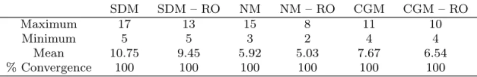
This is not a true MDO problem. We created this problem for visualiza-tion and explanavisualiza-tion purposes: its small size allowed us to illustrate optimiza-tion behaviour and algorithm implementaoptimiza-tion more easily than on higher-dimensional problems. It does not have multiple disciplines, but it has design variables and a state variable defined by a state equation (MDO problems have design variables and multiple state variables defined by state equations); we can solve its state equation in residual form with a root-finding algorithm (as can be done, in principle, with MDO problems); and we can calculate the nec-essary Riemannian optimization quantities using our MDO formulae. As such, it has some of the qualities of an MDO problem, and that makes it useful for an initial demonstration. The optimization results for a calculated step size, line search, and geodesic search are shown in Tables 2, 3, and 4, respectively.
Table 2 Algorithm Iterations to Convergence, Two-Dimensional Illustrative Problem (Cal-culated Step Size)
SDM SDM – RO NM NM – RO CGM CGM – RO
Maximum 17 13 15 8 11 10
Minimum 5 5 3 2 4 4
Mean 10.75 9.45 5.92 5.03 7.67 6.54 % Convergence 100 100 100 100 100 100
Table 3 Algorithm Iterations to Convergence, Two-Dimensional Illustrative Problem (Line Search) SDM SDM – RO NM NM – RO CGM CGM – RO Maximum 16 12 6 8 8 8 Minimum 2 2 2 2 2 3 Mean 8.49 8.04 3.66 3.89 5.03 5.16 % Convergence 100 100 98 98 100 100
Table 2 shows that all of the methods converged for the calculated step size. In this case, the Riemannian algorithms were all somewhat faster than their Euclidean counterparts. As would be expected, SDM was the slowest and NM was the fastest. The results in Table 3, however, now have two nonconverged runs for each of the NM, and although the Riemannian SDM is still slightly faster than Euclidean SDM, the Riemannian NM and CGM are now slightly
Table 4 Algorithm Iterations to Convergence, Two-Dimensional Illustrative Problem (Geodesic Search) SDM SDM – RO NM NM – RO CGM CGM – RO Maximum 15 14 6 10 8 9 Minimum 1 1 2 2 1 1 Mean 8.94 8.16 3.81 4.34 5.30 5.65 % Convergence 100 100 98 96 100 100
slower than the Euclidean versions. We also note that the line search methods are all roughly two iterations faster, on average, than the calculated step size methods. Finally, as we see in Table 4, geodesic search produced results similar to line search in terms of the relative performances of the algorithms, but the geodesic search was slightly slower, across all algorithms, than the line search.
Fig. 3 Euclidean NM Phase Portrait, Two-Dimensional Illustrative Problem
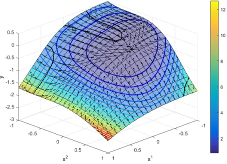
The nonconvergence in NM can be explained by considering the phase por-traits of ˙x=dfor the Euclidean and Riemannian versions; see (Bakker et al. 2013b) for more on the use of ODEs to investigate optimization behaviour. Figure 3 shows the phase portrait for Euclidean NM, and Fig. 4 shows the phase portrait for Riemannian NM: the vectors have been normalized to show direction only, and the thick black lines indicate where the hessian (for Eu-clidean NM) or covariant hessian (for Riemannian NM) is singular. In some cases, the search direction for the algorithm flips directions across these lines.
Fig. 4 Riemannian NM Phase Portrait, Two-Dimensional Illustrative Problem
If the (covariant) hessian is no longer positive definite, the search direction may actually end up being an ascent direction, and this terminates the line and geodesic searches – thus why they terminated without converging.
Moreover, although this did not arise in our tests, it is clear that the calculated step size could fail to converge for the Riemannian NM as it would not for the Euclidean NM. Both algorithms have some areas of the domain where the flow is away from the optimum (i.e. the problem is nonconvex in those regions), but that flow is never directed into one of the corners for NM – near the corners, there is always a component of the flow directed away from that corner. As can be seen in Fig. 4, however, around (x1, x2) = ( 1, 1), the Riemannian NM flow is directed into the corner, and thus the algorithm would terminate there.
4.2 Two-discipline analytical MDO problem The next problem used was
minf =z21+z22 y1+e y2+x21 (35)
y1=x1 x22 z1z2+y32 (36)
y2= x3x4+z1+z22 y1 (37)
This problem is similar in form to, though greater in dimensionality than, the analytical test problem created by Sellar et al. (1996) and used elsewhere (e.g. (Bakker and Parks 2015b; Perez et al. 2004)). Our state equations for disciplines 1 and 2 are in (36) and (37), respectively. If we take them and put them in residual form, we obtain
h= ⇢ h1 h2 = ⇢ y1 x1+x2 2+z1z2 y32 y2+x3x4 z1 z22+y1 =0 (39)
Note how this corresponds to our description in Section 2.3. To reiterate, our optimization algorithm takes steps inw, and the multidisciplinary analysis then solves (39) to calculatey.
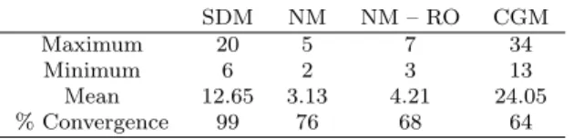
The Euclidean and Riemannian SDM consistently failed to converge for the calculated step size: both produced optimization runs which were apparently chaotic. This can happen with SDM if the step size is too large (van den Doel and Ascher 2012). Table 5 shows the Riemannian versions performing worse than the Euclidean ones in terms of both iterations to convergence and convergence percentage.
Table 5 Algorithm Iterations to Convergence, Two-Discipline Analytical MDO Problem (Calculated Step Size)
NM NM – RO CGM CGM – RO
Maximum 13 11 96 97
Minimum 2 3 11 12
Mean 4.11 4.78 31.68 38.47 % Convergence 95 81 98 72
Table 6 Algorithm Iterations to Convergence, Two-Discipline Analytical MDO Problem (Line Search) SDM NM NM – RO CGM Maximum 20 5 7 34 Minimum 6 2 3 13 Mean 12.65 3.13 4.21 24.05 % Convergence 99 76 68 64
Surprisingly, Riemannian SDM and CGM with line search produced no converged runs. Further investigation showed that the problem lay in the methods’ behaviour at design space boundaries. Consider the diagram in Fig. 5: it shows the search directions f,i and gijf,j pointing outwards into an infeasible region (shaded in grey) along with the projections of those search directions onto the design space boundary. Since gij is positive definite, the angle between f,i and gijf,j is less than 90 . However, in this instance,
Fig. 5 Projections and Direction Splitting on Design Space Boundaries
the directions fall on opposite sides of the constraint normal, so the search directions’ projections point in opposite directions. The projection of f,ihas to be a descent direction, so the projection of gijf,j must be an ascent di-rection and thus the line search terminates the algorithm without converging. The same thing can and does happen with NM. See our comments at the end of Section 5.2 regarding why Riemannian SDM and CGM may be prone to this kind of behaviour. Occasionally, the optimization also failed because the multidisciplinary analysis failed to converge (as with the lone SDM failure in Table 6
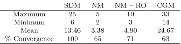
Table 7 Algorithm Iterations to Convergence, Two-Discipline Analytical MDO Problem (Geodesic Search) SDM NM NM – RO CGM Maximum 25 5 10 33 Minimum 6 2 3 14 Mean 13.46 3.38 4.90 24.67 % Convergence 100 65 71 63
As with line search, the Euclidean NM was faster than the Riemannian NM and the Riemannian SDM and CGM completely failed to converge for geodesic search (Table 7). Choosing geodesic search over line search does not a↵ect the initial search direction, and the problem lay in the search direction, not the search method. The geodesic search also produced slightly higher average iterations to convergence than the line search and reduced the convergence percentage in all algorithms save the Riemannian NM.
4.3 Satellite design problem
Here, we employ a satellite design problem as described by Mesmer et al. (2013) 1. A full description is also provided in (Bakker 2015). In lieu of that full description, we provide below a list of the problem’s disciplines in Table 8, a list of design variables in Table 9, a list of state variables in Table 10, and a Design Structure Matrix (DSM) (Browning 2001) in Table 11 to qualitatively indicate the problem’s structure.
Table 8 Satellite Design Problem Disciplines
Discipline Number
Payload 1
Propulsion 2
Power 3
Attitude Determination and Control Systems (ADCS) 4
Thermal 5
Structures 6
Table 9 Satellite Design Problem Design Variables
Symbol Description Discipline(s) Used
fdown Downlink Frequency 1
fup Uplink Frequency 1
Pt Satellite Transmitter Power 1
Pgt Ground Transmitter Power 1
Dgr Ground Receiving Antenna Diameter 1
Dgt Ground Transmitting Antenna Diameter 1
✏ Battery Energy Density 3
Dst Satellite Transmitting Antenna Diameter 1,4,5
Dsr Satellite Receiving Antenna Diameter 1,4,5
We use total mass, total cost, and the weighted sum of total mass and Signal-to-Noise Ratio (SNR) (appropriately normalized) as the three di↵erent objectives under consideration. Because of the increased computational cost of running these optimizations, however, we limited our runs to 20 iterations and forewent the geodesic search; some of the optimization runs took over an hour, and in our previous problems, the geodesic search could take an order of magnitude longer than the line search. Geodesic search was consistently worse than line search in our previous results, so we felt justified in omitting the geodesic search on this problem.
The calculated step size optimizations on the total mass all failed to con-verge except for the Riemannian SDM and CGM runs, as seen in Table 12; 1 The problem description is too lengthy to include here, but full details of the satellite
design problem are available from the authors upon request.
Table 10 Satellite Design Problem State Variables
Symbol Description Discipline of Origin
SN R Signal-to-Noise Ratio 1
Mst Satellite Transmitting Antenna Mass 1
Msr Satellite Receiving Antenna Mass 1
Mtransp Transponder Mass 1
Mpayload Payload Mass 1
Ppayload Payload Power Requirement 1
Vtransp Transponder Volume 1
Mprop Propellant Mass 2
Vprop Propellant Tank Volume 2
MSA Solar Array Mass 3
AS Solar Array Area 3
Mbatt Battery Mass 3
Vbatt Battery Volume 3
MADCS ADCS Mass 4
PADCS ADCS Power Requirement 4
VRW Reaction Wheel Volume 4
Mthermal Thermal System Mass 5
Pthermal Thermal System Power Requirement 5
Ls Satellite Bus Length 6
rs Satellite Bus Radius 6
ts Satellite Bus Thickness 6
Mbus Satellite Bus Mass 6
Table 11 Satellite Design Problem DSM
1 2 3 4 5 6 1 X • • • • • 2 X • • • 3 • X • • • 4 • • X • • 5 • • • X • 6 • • • X
Table 12 Algorithm Iterations to Convergence, Satellite Design Problem, Total Mass (Cal-culated Step Size)
SDM – RO CGM – RO
Maximum 15 16
Minimum 5 5
Mean 9.42 9.70
% Convergence 98 97
the handful of nonconverged runs for those algorithms failed because they pro-duced points where the multidisciplinary analysis failed to produce a feasible design. Euclidean SDM and CGM, on the other hand, went immediately to the design space boundaries and then began taking very short steps until they ran out of iterations. As for NM, the Riemannian version diverged o↵into a corner of the design space because the covariant hessian was not positive definite –
the negative eigenvalues of the covariant hessian were sometimes an order of magnitude larger than its positive eigenvalues – and the Euclidean NM failed to calculate a search direction because the hessian was singular everywhere.
Table 13 Algorithm Iterations to Convergence, Satellite Design Problem, Total Mass (Line Search) SDM SDM – RO CGM CGM – RO Maximum 4 8 4 8 Minimum 4 5 4 5 Mean 4 6.71 4 6.48 % Convergence 100 100 100 100
The results in Table 13 for line search optimizations, however, were rather di↵erent. Euclidean NM still failed to calculate a search direction, and Rieman-nian NM still produced ascent search directions because the covariant hessians were not positive definite; SDM and CGM both performed much better. The Euclidean SDM and CGM both required significant computational time but few iterations. The algorithms would begin from an unconstrained point and then reach a new variable bound at each iteration until they finally ended up at the optimum. The nature of the problem enabled Euclidean SDM and CGM to do this, and that is why they always took four iterations to converge.
The total cost objective was more complicated than the total mass func-tion, and this increased complexity is likely why none of the calculate step size algorithms converged. With the line search (results shown in Table 14), Riemannian and Euclidean NM failed for the same respective reasons as they did with the total mass objective, and Euclidean SDM and CGM displayed the same behaviour as before but with seven iterations rather than four. Rieman-nian SDM failed on nine occasions due to either direction splitting or running out of iterations, but in 80% of the runs, it took nine iterations to converge in a manner similar to SDM, CGM, and Riemannian CGM.
Table 14 Algorithm Iterations to Convergence, Satellite Design Problem, Total Cost (Line Search) SDM SDM – RO CGM CGM – RO Maximum 7 20 7 9 Minimum 7 9 7 9 Mean 7 9.62 7 9 % Convergence 100 91 100 100
Following these trials, we ran optimizations on the weighted sum of the total mass and SNR. This objective, unlike the previous two, did not have a singular hessian everywhere in the design space. However, it also produced no Riemannian Optimization in Multidisciplinary Design Optimization 23
converged runs. The hessian was not singular, but it was not positive definite, and as a result, the Riemannian and Euclidean NM diverged for the calculated step size. When using line search, they terminated when the search direction became an ascent direction (within the first few iterations in all NM cases). Euclidean SDM and CGM typically ran out of iterations without converging for both line search and calculated step size because their progress at each iteration was very small. The Riemannian versions using a calculated step size failed in a similar fashion; they failed by direction splitting or running out of iterations when using line search. All of the algorithms occasionally ended up at points with nonconverged multidisciplinary analyses.
That being said, Riemannian SDM and CGM did get very close to converg-ing on a number of occasions: the convergence criterion was that the norm of the projected gradient had to be less than 10 3, and several of the runs would have counted as converged if the criterion had been less strict, as shown in Ta-ble 15. In these cases, the di↵erence in objective function value between these runs and the true optimum was less than 0.5%. The algorithms appeared to have failed at this point due to direction splitting. The objective function derivatives in the satellite design problem were, in general, of much greater magnitudes than in the previous problems. Given that, and given the fact that the runs recorded in Table 15 all produced objective function values which were extremely close to the true optimum, it may be that the convergence criterion was more strict than necessary here.
Table 15 Percentage of Nearly Converged Runs, Satellite Design Problem, Weighted Sum Objective (Line Search)
Convergence Criterion SDM – RO CGM – RO
<0.1 7 9
<0.01 5 7
5 Discussion
5.1 Optimization results
Geodesic search was not as e↵ective as line search. We knew ahead of time that it would be more expensive to implement, but if it provided better perfor-mance, it might be worth developing a computationally cheaper approxima-tion. However, such an e↵ort would not seem to be justified. Furthermore, al-though the Riemannian algorithms were sometimes better than the Euclidean ones when using a calculated step size, the Euclidean algorithms were generally better overall when line search or geodesic search was used.
Both Euclidean and Riemannian NM diverged on the satellite design prob-lem objective functions, but they did so in di↵erent ways – the covariant
hessian was not singular when the hessian was, and in other optimization problems, that could be an advantage. Riemannian SDM and CGM had con-vergence problems because of direction splitting, however. Their concon-vergence problem was due to the way in which the constraints were handled: penalty functions, for example, might have enabled the algorithms to avoid this prob-lem. If this difficulty were overcome, the Riemannian version could be more e↵ective as the weighted sum satellite design results hinted at. Feasible direc-tions is a standard method and easy to implement, though, and it is particu-larly convenient for simple bounds on design variables. On other test problems, which we did not present here, we also found that the Riemannian algorithms had greater difficulties with ill-conditioning in @h
@y due to the presence of g
ij and i
jk.
Given that the Riemannian algorithms are likely to have a higher cost per iteration than the Euclidean algorithms, it would seem that the Euclidean methods are better than the Riemannian ones as we have developed them here. That being said, real-world phenomena, such as nonconvexity, in our satellite design problem made it difficult for any of the algorithms to converge. Final conclusions on the relative performances of Riemannian and Euclidean algorithms would require comparisons with algorithms sophisticated enough to converge reliably on such problems.
5.2 Riemannian optimization and design coupling
We now wish to analyze the algorithms themselves further for any a priori performance information which we might glean. In particular, we would like to look at the algorithms’ interaction with design coupling and direction splitting. Previously, we identified two di↵erent schools of thought on measuring design coupling: one focuses on design structure (i.e. the number and arrangement of variables and functions) in its evaluation of coupling, whereas the other uses design sensitivity information, and they put their respective measures of coupling to di↵erent uses (Bakker et al. 2013a); our paper on design coupling provides more detail on each school and their approach to design coupling
Here, we will focus on sensitivity-based coupling – coupling that measures how strongly the state variables depend on the design variables. Sensitivity-based coupling changes throughout the design space, unlike structure-Sensitivity-based coupling, but we are now also making a slight innovation by considering how sensitivity changes withsearch directionas well as location. In other words,@@wy varies aswchanges, but we will also consider how the choice ofd(k)interacts with @@wy.
We begin by stepping out of Riemannian geometry briefly to examine the matrix gij and its eigenvalues. Consider a vector in the design space w of unit length (i.e. wi wi= 1). The (first-order approximation to the) change in the state variables corresponding to this vector is
y= @y @w w (40) which is equivalent to yi = @y i @wj w j (41)
Using the knowledge that gij = ij+@y
k
@wi
@yk
@wj, we can see that
wigij wj = wi wi+ yi yi = 1 + yi yi (42) In matrix notation, g=I+h@@wyiTh@@wyi, so
wTg w= wT w+ yT y= 1 + yT y (43)
Therefore, the eigenvalues ofgijare all greater than or equal to one. Eigen-vectors with eigenvalues equal to one will be in directions of constantyon the manifold, and eigenvectors with large associated eigenvalues will be in direc-tions of large change in the state variables.
If the eigenvalues of gij are greater than or equal to one, then the eigen-values ofgij are less than or equal to one, and thus g 1 w
k wk. More specifically, if iis an eigenvalue forgijand⇠iis its corresponding (normalized) eigenvector, the eigenvectors are all mutually orthogonal (becausegij is sym-metric), and we can represent w as w =P
i ↵i⇠i, where k wk2 =P i ↵2 i. With this representation,
g 1 w=X i ↵i i ⇠i (44) g 1 w 2=X i ↵2 i i2 k wk2=X i ↵2i (45)
In other words, multiplying a vector (we ignore the distinction between vectors and covectors here) by g 1 will never result in an increase – and typically will result in a decrease – in vector magnitude. Furthermore, even if
g 1 w is re-normalized so that its norm is the same as the original w, the new vector will have had its direction changed from the original one, and the new direction will be “less coupled” than the original one: as (44) shows, the multiplication by g 1 shrinks the vector in directions of large change in the state variables proportionate to the degree of that change (represented by i). “Uncoupled directions” – directions of constanty – are left unchanged.
We can see, therefore, that the Riemannian versions of SDM and CGM will always have “flatter” trajectories, with respect toy, than their Euclidean counterparts. Figure 6 shows an example of this: the black path corresponds to ˙xi = f,i, and the light grey path corresponds to ˙xi = gijf,j. The trend
is easier to see in the di↵erential equation rather than the original iterative algorithm; see Bakker et al. (2013b) for more on the use of di↵erential equations in analyzing optimization algorithms.
Fig. 6 Riemannian and Euclidean ODE Trajectories
We can further see that direction splitting will be a problem if a strong change inycorresponds to a decrease in the objective function along a bound-ary: gijf,j will point further away from f,i under such circumstances and thus be more likely to be caught on the wrong side of the constraint nor-mal. The satellite design problem’s objective functions, for example, depend strongly on the state variables, and this may explain the poor performance of the Riemannian algorithms there. Even when the algorithms did not termi-nate as a result of direction splitting, moving in less coupled directions would have meant less change in the objective function and thus why more iterations would have been required even when the algorithms did converge. Conversely, we can say that Riemannian SDM or CGM could be particularly e↵ective on problems where it would be advantageous for the optimization trajectory to be “flatter” with respect to the state variables.
Although we have not come across particular design problems where this is the case, this may still be valuable information in light of the No Free Lunch (NFL) theorem (Wolpert and Macready 1997). According to the NFL theorem, no one algorithm is better than another when their respective per-formances are averaged over all possible optimization problems. As such, the key to improved optimization lies in being able to say, a priori, when one Riemannian Optimization in Multidisciplinary Design Optimization 27
optimization algorithm will be better than anotheron a given problem. Our analysis of coupling suggests that Riemannian SDM and CGM will perform better than their Euclidean counterparts on problems where it is beneficial to have less variation in the state variables over the course of the optimization. Similarly, the results of that analysis, combined with our experimental results, show that the Euclidean versions will be better on problems where the objec-tive function varies strongly with the state variables and the optimum lies on the design space boundary.
Unfortunately, NM is not amenable to similar analysis. Here, we begin fromf;ij instead ofgij, and we can break it up into componentsf;ij =f,ij
k
ijf,k. However, the ijkf,kterm, which determines the di↵erence between the Euclidean and Riemannian trajectories, does not have a simple representation in terms of implicit derivatives:
k ijf,k= gkm @ys @wm @2ys @wi@wjf,k (46)
Asf,kgoes to zero, the Euclidean and Riemannian trajectories will become more and more similar, but beyond that, there is little to say in terms of general statements.
5.3 Riemannian optimization in the broader context of MDO
RO algorithms are simply di↵erent versions of standard gradient-based opti-mization algorithms, and as such, they are similarly general within an MDO context. These algorithms are not part of the decomposition process – that is handled by the architecture. As with standard gradient-based algorithms, RO algorithms can then be applied to the problem after the architecture has been implemented (e.g. MDF with Riemannian CGM, or regular CGM, or an-other algorithm entirely). In principle, the Riemannian algorithms described and tested here can be applied wherever gradient-based algorithms are al-ready used in MDO; a Riemannian quasi-NM algorithm could be used where a quasi-NM algorithm is currently being used, for example.
The presence of potentially di↵erent architectures does add some complex-ity, however. Riemannian algorithms require a metric tensor and Christo↵el symbols (which are themselves produced from basic sensitivity information). As we have shown elsewhere (Bakker et al. 2012), MDF uses the original feasible design manifold, and thus the metric tensor and Christo↵el symbols used with MDF are the metric tensor and Christo↵el symbols for the original problem. The decompositions involved in MDO architectures alter the original manifold, though. To be more precise, the optimization processes in the dif-ferent architectures occur on di↵erent manifolds – ones which are created by the decomposition process. This means that the metric tensors and Christo↵el symbols will be calculated with di↵erent formulae than were shown here. How-ever, we have already calculated those metric tensors and Christo↵el symbols
from basic sensitivity information for six di↵erent MDO architectures else-where (Bakker et al. 2012). Those calculations could be done, in principle, for any other architecture of interest, as well. In other words, the search direction for the Riemannian SDM will still be
dj= gijf,i (47)
but thegij needed to determinegij will not be calculated using (12). We show how to calculategij for those other architectures in (Bakker et al. 2012).
RO algorithms have the same strengths and weaknesses as other gradient-based methods have in comparison to metaheuristic or hybrid methods. The comparative capabilities and limitations of gradient-based, metaheuristic, and hybrid methods, in general, are well-known. The comparative capabilities and limitations ofRiemannian and standard Euclidean methods on MDO problems are the subject of our inquiry here.
Lest it need be said again, RO algorithms are just like regular gradient-based algorithms. The two di↵erences lie in the modified derivative information (e.g. the covariant derivative vs. a regular gradient) and the modified search path (along geodesics vs. along straight lines). Any di↵erences in behaviour may be traced to those two properties; in all other respects, they are the same. The burden of this paper has been to compare these single-objective, gradient-based methods in terms of their efficiency, measured by the number of iterations to convergence, and their e↵ectiveness, measured by their percent convergence.
RO methods could therefore be incorporated into hybrid optimization methods anywhere in MDO that standard gradient-based algorithms currently are. To be even more general, the modified derivative information used in RO could be used anywhere that regular derivative information currently is, and the modified search direction used in RO could be used in some of the places where line searches currently are; the need for derivative information to calculate geodesics limits geodesic search as compared to line searches. How-ever, implementing RO algorithms on MDO and comparing them with other gradient-based algorithms, as we have done in this paper, is both logically and chronologically prior to any extensions into hybrid optimization methods.
5.4 Recommendations and future work
We have shown our Riemannian optimization algorithms to be less efficient and less e↵ective, on the whole, than their Euclidean counterparts. In or-der to be sure of Euclidean superiority, however, we would need to develop and test a Riemannian quasi-NM (the various implementations of quasi-NM form a standard against which other gradient-based algorithms are measured), consider di↵erent methods for handling inequality constraints, and test on a wider range of MDO problems. We also showed line searches to be better than geodesic searches on our test problems. That being said, the results for any Riemannian algorithm will depend on the metric being used: both the search Riemannian Optimization in Multidisciplinary Design Optimization 29
directions and the geodesics depend on the metric (for a metric-compatible connection). We used the induced metric, but other metrics could prove to be more favourable. It could also be beneficial to look into convexifying the original optimization problem through the imposition of a particular metric. In Section 2.5, we mentioned this being done elsewhere, but we did not go into detail about how this might profitably be applied to MDO. Finally, our analysis of the search directions and their relationship to design coupling for Riemannian SDM and CGM was informative, and it might be similarly in-formative to analyze geodesic trajectories to further explain our performance results.
6 Summary
We began our paper by reviewing the background theory for our MDO dif-ferential geometry framework, the additional theory necessary for doing RO, and the RO literature. Given the historical lack of crossover between RO and MDO, we considered this to be particularly important in presenting our re-sults to the MDO community. With this in place, we showed how to apply RO algorithms to MDO through the use of our framework.
We then tested some of these algorithms on MDO problems using our di↵erential geometry framework’s induced metric. Our results here showed geodesic search to be consistently less e↵ective than line search, and the RO algorithms were generally not as good as the Euclidean algorithms when us-ing a feasible directions method to handle inequality constraints. That beus-ing said, the Riemannian SDM and CGM with calculated step size proved to be a stark exception to this trend when applied to one version of our satellite design problem: they significantly outperformed the Euclidean algorithms in that case. The covariant hessian was also nonsingular in many cases when the regular hessian was singular, so the Riemannian NM was often able to calcu-late a step direction when the Euclidean NM could not. The nonconvexity we encountered, however, demonstrated the need to compare performance with more robust optimization algorithms (like quasi-NM) and using additional test problems for more conclusive results.
Through our analysis of the algorithms themselves, we showed how the Rie-mannian SDM and CGM interact with design coupling: they produce steps in directions which are less strongly coupled than their Euclidean counterparts. This has provided us with some ability to predict the performance of those methods relative to each other based on a priori information about the rela-tionship between the state variables and the objective function.
Most importantly, we have now set the stage for further investigation into the application of RO to MDO – we have shown boththat it can be done and how it may be done. Our preliminary work here in reviewing, testing, and an-alyzing RO methods, moreover, has pointed out avenues of future exploration in this area.
Acknowledgments
This research is supported by the Natural Sciences and Engineering Research Council of Canada (NSERC) and the Cambridge Trusts. The authors would also like to thank Mr. Hanumanthrao Kannan for his assistance in setting up the satellite design problem.
References
Allison JT, Herber DR (2013) Multidisciplinary design optimization of dy-namic engineering systems. In: 54thAIAA/ASME/ASCE/AHS/ASC Struc-tures, Structural Dynamics, and Materials Conference, AIAA, Boston, Mas-sachusetts
Baker CG (2008) Riemannian manifold trust-region methods with applications to eigenproblems. PhD thesis, Florida State University, Tallahassee, Florida Bakker C (2015) A di↵erential geometry framework for multidisciplinary de-sign optimization. PhD thesis, University of Cambridge, Cambridge, United Kingdom
Bakker C, Parks GT (2015a) Di↵erential geometry tools for multidisciplinary design optimization, part I: Theory. Structural and Multidisciplinary Opti-mization 52:27–38
Bakker C, Parks GT (2015b) Di↵erential geometry tools for multidisciplinary design optimization, part II: Application to QSD. Structural and Multidis-ciplinary Optimization 52:39–53
Bakker C, Parks GT, Jarrett JP (2012) Geometric perspectives onMDOand MDOarchitectures. In: 12th Aviation Technology, Integration and Opera-tions (ATIO) Conference and 14thAIAA/ISSMO Multidisciplinary Analysis and Optimization Conference, AIAA, Indianapolis, Indiana
Bakker C, Parks GT, Jarrett JP (2013a) Di↵erential geometry and design cou-pling inMDO. In: 54th AIAA/ASME/ASCE/AHS/ASC Structures, Struc-tural Dynamics, and Materials Conference, AIAA, Boston, Massachusetts Bakker C, Parks GT, Jarrett JP (2013b) Optimization algorithms andODE’s
in MDO. In: ASME 2013 Design Engineering Technical Conferences and Computers and Information in Engineering Conference, ASME, Portland, Oregon
Barthelemy JFM, Sobieszczanski-Sobieski J (1983) Extrapolation on optimum design based on sensitivity derivatives. AIAA Journal 21:797–799
Bento GC, Ferreira OP, Liveira PR (2012) Unconstrained steepest descent method for multicriteria optimization on Riemannian manifolds. Journal of Optimization Theory and Applications 154:88–107
Boothby WM (1986) An Introduction to Di↵erentiable Manifolds and Rieman-nian Geometry. Academic Press, Inc., Boston
Browning TR (2001) Applying the design structure matrix to system decompo-sition and integration problems: A review and new directions. IEEE Trans-action on Engineering Management 48:292–306