Simultaneous Localisation and Mapping (SLAM):
Part II State of the Art
Tim Bailey and Hugh Durrant-Whyte
Abstract— This tutorial provides an introduction to theSi-multaneous Localisation and Mapping (SLAM) method and the extensive research on SLAM that has been undertaken. Part I of this tutorial described the essential SLAM prob-lem. Part II of this tutorial (this paper) is concerned with recent advances in computational methods and in new for-mulations of the SLAM problem for large scale and complex environments.
I. Introduction
SLAM is the process by which a mobile robot can build a map of the environment and at the same time use this map to compute it’s location. The past decade has seen rapid and exciting progress in solving the SLAM problem together with many compelling implementations of SLAM methods. The great majority of work has focused on im-proving computational efficiency while ensuring consistent and accurate estimates for the map and vehicle pose. How-ever, there has also been much research on issues such as non-linearity, data association and landmark characterisa-tion, all of which are vital in achieving a practical and robust SLAM implementation.
This tutorial focuses on the recursive Bayesian formula-tion of the SLAM problem in which probability distribu-tions or estimates of landmark locadistribu-tions and vehicle pose are obtained. Part I of this tutorial surveyed the develop-ment of the essential SLAM algorithm in state-space form, described a number of key implementations and cited lo-cations of source code and real-world data for evaluation of SLAM algorithms. Part II of this tutorial (this paper) surveys the current state of the art in SLAM research with a focus on three key areas; computational complexity, data association, and environment representation. Much of the mathematical notation and essential concepts used in this paper are defined in Part I and so are not repeated here.
SLAM, in it’s naive form, scales quadratically with the number of landmarks in a map. For real-time implemen-tation, this scaling is potentially a substantial limitation in the use of SLAM methods. Section II surveys the many approaches that have been developed to reduce this complexity. These include linear-time state augmentation, sparsification in information form, partitioned updates and submapping methods. A second major hurdle to overcome in implementation of SLAM methods is to correctly as-sociate observations of landmarks with landmarks held in
Tim Bailey and Hugh Durrant-Whyte are with the Aus-tralian Centre for Field Robotics (ACFR) J04, The University of Sydney, Sydney NSW 2006, Australia, [email protected], [email protected]
the map. Incorrect association can lead to catastrophic failure of the SLAM algorithm. Data association is par-ticularly important when a vehicle returns to a previously mapped region after a long excursion; the so-called ‘loop-closure’ problem. Section III surveys current data as-sociation methods used in SLAM. These include batch-validation methods that exploit constraints inherent in the SLAM formulation, appearance-based methods, and multi-hypothesis techniques. The third development discussed in this tutorial is the trend towards richer appearance-based models of landmarks and maps. While initially motivated by problems in data association and loop closure, these methods have resulted in qualitatively different methods of describing the SLAM problem; focusing on trajectory esti-mation rather than landmark estiesti-mation. Section IV sur-veys current developments in this area along a number of lines including delayed mapping, the use of non-geometric landmarks, and trajectory estimation methods.
SLAM methods have now reached a state of consider-able maturity. Future challenges will centre on methods enabling large scale implementations in increasingly un-structured environments and especially in situations where GPS-like solutions are unavailable or unreliable; in urban canyons, under foliage, underwater or on remote planets.
II. Computational Complexity
The state-based formulation of the SLAM problem in-volves the estimation of a joint state composed of a ro-bot pose and the locations of observed stationary land-marks. This problem formulation has a peculiar structure; the process model only affects vehicle pose states and the observation model only makes reference to a single vehicle-landmark pair. A wide range of techniques have been de-veloped to exploit this special structure in limiting the com-putational complexity of the SLAM algorithm.
Techniques aimed at improving computational efficiency may be characterised as being optimal or conservative. Optimal algorithms aim to reduce required computation while still resulting in estimates that are equal to the full-form SLAM algorithm (as presented in Part I of this tu-torial). Conservative algorithms result in estimates which have larger uncertainty or covariance than the optimal re-sult. Usually conservative algorithms, while less accurate, are computationally more efficient and therefore of value in real implementations. Algorithms with uncertainties or covariances less than those of the optimal solution are termed inconsistent and are considered invalid solutions to the SLAM (or any estimation) problem.
The direct approach to reducing computational complex-ity involves exploiting the structure of the SLAM problem in re-formulating the essential time and observation up-date equations. The time-upup-date computation can be lim-ited using state-augmentation methods. The observation-update computation can be limited using apartitioned form
of the update equations. Both these steps result in an op-timal SLAM estimate with reduced computation. Refor-mulation of the standard state-space SLAM representation into information form allowssparsificationof the resulting information matrix to be exploited in reducing computa-tion. Both optimal and conservative variations exist of these sparsification algorithms. Submapping methods ex-ploit the idea that a map can be broken up into regions with local coordinate systems and arranged in a hierarchi-cal manner. Updates occur mostly in a lohierarchi-cal frame with periodic inter-frame updates. Submapping techniques gen-erally provide a conservative estimate in the global frame.
A. State Augmentation
At a time k, the joint SLAM state vector xk = [xTvk,mT]T comprises two parts; the robot pose xvk and the set of map landmark locations m. The vehicle model propagates only the pose states according to a set of control inputsuk while leaving the map states unchanged:
xk =f(xk−1,uk) = fvxvk−1,uk m (1)
In a naive implementation of the extended Kalman filter (EKF) for SLAM, the covariance prediction is computed from
Pk|k−1=∇fx Pk−1|k−1∇fxT+∇fuUk∇fuT (2) where ∇fx = ∂xk∂f
−1, ∇fu =
∂f
∂uk and Uk is a covariance characterising uncertainty on the control vector. This op-eration has cubic complexity in the number of landmarks due to matrix multiplication of the Jacobian∇fx and the covariance matrix Pk−1|k−1. However, as only the pose states are affected by the vehicle model, the covariance prediction can be re-written in a form which has linear complexity in the number of landmarks [56, Section 2.4.1]:
Pk|k−1= ∇fvx Pvv∇fvTx+∇fvu Uk∇fvTu ∇fvx Pvm PTvm∇fvTx Pmm (3) where∇fvx =∂x∂fvvk−1,∇fvu =∂uk∂fv and where
Pk−1|k−1=
Pvv Pvm PTvm Pmm
The process of adding a new landmark to the state vector has a similar form. A new map landmark is initialised as a function of the robot pose and an observationzk.
mnew=g(xvk,zk) (4)
The augmented states are then a function of only a small number of existing states
x+k = ⎡ ⎣ xmvk g(xvk,zk) ⎤ ⎦ (5)
The general idea of state augmentation can be applied whenever new states are a function of a subset of existing states ⎡ ⎣ xx12 f(x2,q) ⎤ ⎦ (6) ⎡ ⎣ P11 P12 P12∇f T x2 PT12 P22 P22∇fxT2 ∇fx2PT12 ∇fx2P22 ∇fx2P22∇fxT2+∇fqQ∇fqT ⎤ ⎦ (7) A comparison of Equations 1 and 3 with Equations 6 and 7, show that the SLAM prediction step is a special case of state augmentation; in which the state is augmented by the new pose xvk, and where the previous pose xvk−1 is then removed by marginalisation. In this form, both the EKF prediction step and the process of adding new landmarks can be reduced to calculations that are linear in the number of landmarks. The resulting estimates are clearly optimal.
B. Partitioned Updates
A naive implementation of the SLAM observation-update step observation-updates all vehicle and map states every time a new measurement is made. For an EKF update, the com-putational effort scales quadratically with the number of landmarks held in the map. A number of partitioned up-date methods have been devised to reduce this computa-tional effort. These confine sensor-rate updates to a small local region and update the global map only at a much lower frequency. These partition methods all produce op-timal estimates.
There are two basic types of partitioned update. The first operates in a local region of the global map and main-tains globally referenced coordinates. This approach is taken by the compressed EKF (CEKF) [23] and the post-ponement algorithm [30]. The second generates a short-term submap with its own local coordinate frame. This is the approach of the constrained local submap filter (CLSF) [56] and the local map sequencing algorithm [47]. We focus on this latter approach as it is simpler and, by performing high-frequency operations in a local coordinate frame, it avoids very large global covariances and so is more numer-ically stable and less affected by linearisation errors.
The local submap algorithm maintains at all times two independent SLAM estimates
xG= xGF mG , xR= xRv mR , (8) wherexGis a map composed of a set of globally referenced landmarks mG together with the global reference pose of
a submap coordinate framexGF, and wherexR is the local submap with a locally referenced vehicle pose xRv and lo-cally referenced landmarks mR as shown in Figures 1(a) and 1(b), respectively.
(a)Global map (b)Local map
(c)Global registration
Fig. 1. The constrained local submap filter. The SLAM frontier is constructed in a local map (b) which periodically registers with a global map (a) to produce an optimal global estimate (c).
As observations are made, conventional SLAM updates are performed entirely within the local submap and with only those landmarks held in the local submap. At any time, a (conservative) global vehicle pose estimate may be obtained cheaply by vector summation of the locally refer-enced pose and the global estimate of the submap coordi-nate frame
xGv =xGF⊕xRv. (9) An optimal global estimate is obtained periodically by reg-istering the submap with the global map, see Figure 1(c), and applying constraint updates upon any features com-mon to both maps. After registration, a new submap is created and the process continues.
The submap method has a number of advantages. First, the number of landmarks that need to be updated at any one time is limited to only those that are described in the local submap coordinate frame. Thus, the sensor-rate up-date is independent of the total map size. The full upup-date, and propagation of local estimates, can be carried out as a background task at a much lower update rate while still permitting sensor-rate global localisation. A second advan-tage is that there is lower uncertainty in a locally referenced frame so approximations due to linearisation are reduced.
Finally, submap registration can use batch validation gat-ing, so improving association robustness.
C. Sparsification
Conventional EKF-SLAM produces a state estimate ˆxk
and covariance matrixPkwhich implicitly describe the first two central moments of a Gaussian probability density on the true state xk. An alternative representation for this same Gaussian is in canonical or information form using the information vector ˆyk and information matrixYk. These are related to the moment form parameters as
Yk =P−k1 (10)
ˆ
yk=Ykxˆk (11)
The advantage of the information form for SLAM is that, for large-scale maps, many of the off-diagonal components of thenormalised information matrix are very close to zero. Thrun et al. [49], [50] have exploited this observation to propose a sparsification procedure which allows near zero elements of the normalised information matrix to be set to zero. With the information matrix now sparse, very efficient update procedures for information estimates can be obtained with relatively little loss in optimality of the maps produced. Although this initial solution was subse-quently shown not to be consistent by Eusticeet al. [19], the idea of sparsification has sparked considerable interest in the information form SLAM problem and several con-sistent sparse solutions [44], [21], [20], [52], [14], [55] have been presented. Of particular note are those solutions that are optimal and exactly sparse [21], [20], [14].
The key to an exactly sparse information form of the SLAM problem is to notice that state augmentation is a sparse operation. Consider the moment-form augmenta-tion identity in Equaaugmenta-tions 6 and 7. These have an equiva-lent information-form identity,
⎡ ⎣ y2− ∇fxT2Q−1[fy(1x2,q)− ∇fx2x2] Q−1[f(x2,q)− ∇fx2x2] ⎤ ⎦ (12) ⎡ ⎣ YY1112T Y22+∇YfxT122Q−1∇fx2 −∇fxT02Q−1 0 −Q−1∇fx2 Q−1 ⎤ ⎦ (13) where, to simplify notation, we assume here thatf(x2,q) =
f(x2) +q. For generality, replaceQ−1with (∇fqQ∇fqT)−1. If the subset of states x1 comprises the bulk of the state vector, then the augmentation in Equation 13 is sparse and has constant-time complexity; compare this to Equation 7 which has linear complexity in the dimension ofx1.
Therefore, in the information form SLAM problem, an exactly sparse solution can be obtained by augmenting the state with the new vehicle pose estimate at each time-step and retaining all past robot poses,
xk = [xTvk,xTvk−1, . . . ,xTv1,mT]T. (14) In this way, the off-diagonal terms of the information ma-trix are non-zero only for poses and landmarks that are
(a)No marginalisation (b)Partial marginalisation (c)Full marginalisation
Fig. 2. Exact information matrix SLAM. These information matrices all represent the same optimal map estimate, but show the tradeoff between number of retained pose states and matrix sparsity. Removing pose states reduces the total matrix size but introduces dependencies between the remaining pose and map states.
directly related by measurement data (see Figure 2(a)). Observation updates are also a sparse operation, produc-ing links only between measured states.
However, marginalisation, which is necessary to remove past pose states, introduces links between all state elements connected to the removed states. Marginalising all past states produces a dense information matrix as shown in Figure 2(c). Nevertheless, it is possible to retain a reason-ably sparse estimate without having to keep an entire pose history [21]. By judicious selection of anchoring poses to decouple different regions of the map, a great proportion of poses can be marginalised away without inducing excessive density as shown in Figure 2(b).
Despite the attraction of its sparse representation, there remain caveats with regard to practical implementation of information form SLAM. For realistic use, it is necessary to recover the mean and covariance of portions of the state at every timestep. This is potentially very expensive. The mean estimate is required to perform linearisation of the process and observation models. It can be recovered fairly efficiently using the conjugate gradients method [18]. The mean and covariance are both required to compute vali-dation gates for data association. While efficient solutions have been devised for simple gating [50], [18], the robust batch gating methods described in Section III potentially involve recovery of the full covariance matrix, which has a cubic complexity in the number of landmarks.
D. Global Submaps
Submap methods are another means of addressing the is-sue of computation scaling quadratically with the number of landmarks during measurement updates. Submap meth-ods come in two fundamental varieties: globally referenced and locally referenced as shown in Figure 3. The common thread to both types is that a submap defines a local co-ordinate frame and nearby landmarks are estimated with respect to the local frame. The local submap estimates are obtained using the standard, optimal SLAM algorithm using only the locally referenced landmarks. The resulting submap structures are then arranged in a hierarchy leading to a computationally efficient suboptimal global map.
(a)Globally referenced submaps
(b)Locally referenced submaps
Fig. 3. Global and relative submaps. Global submaps share a com-mon base coordinate frame while relative submaps record only relative poses of neighbouring frames.
Global submap methods estimate the global locations of submap coordinate frames relative to a common base frame. This is the approach adopted in the relative land-mark representation (RLR) [24] and constant time SLAM (CTS) [32] methods. These approaches reduce computa-tion from a quadratic dependence on number of landmarks, to a linear or constant time dependence by maintaining a conservative estimate of the global map. However, as submap frames are located relative to a common base coor-dinate frame, global submaps do not alleviate linearisation issues arising from large pose uncertainties [4].
E. Relative Submaps
Relative submap methods differ from global submaps in that there is no common coordinate frame. The location of any given submap is recorded only by its neighbour-ing submaps, and these are connected in a graphical net-work. Global estimates can be obtained by vector summa-tion along a path in the network. By eschewing any form of global-level data fusion, relative submaps address both computation and non-linearity issues.
The original notion of relative submaps was introduced by Chong and Kleeman [9]. This was further developed by Williams [56] in the form of the constrained relative submap filter (CRSF). However, CRSF does not exhibit global level convergence without forfeiting the decoupled submap structure. The Atlas framework [7], [8] and net-work coupled feature maps (NCFM) [2] rectified this prob-lem by realising that conservative global convergence could be achieved using the covariance intersect algorithm [28] for estimating connections. Another solution, called hier-archical SLAM [17], increases the global convergence rate by imposing loop constraints whenever the vehicle closes a loop. These algorithms result in a network of optimal SLAM submaps connected by conservative links.
The relative submap framework has a number of advan-tages. In particular, it produces locally optimal maps with computational complexity independent of the size of the complete map. Further, by treating updates locally it is numerically very stable, allows batch association between frames and minimises problems arising from linearisation in a global frame.
F. Mapping Relative Quantities
Almost all practical SLAM algorithms are built upon an absolute or global map framework. Even those that construct a system of submaps treat each local coordinate frame as a small absolute map. The essence of an absolute map is a base coordinate frame that defines the map origin and all landmarks and the robot pose are referenced with respect to this frame.
An alternative map representation is a relative map, in-troduced by Csorba [11], where, rather than estimate land-mark locations, the SLAM state is composed of distances and angles between landmarks. The advantage of this form is an uncorrelated state estimate, which permits constant-time computation. The problem, however, is that a relative map does not directly represent location and recovering ve-hicle pose is non-trivial. There are also practical issues with implementing observation models and data association.
Due to these limitations relative maps have not gained wide acceptance. However, there has been a recent resur-gence in interest with D-SLAM [54] and Julier’s multiple maps [29] making use of the relative map representation.
III. Data Association
Data association has always been a critical issue for prac-tical SLAM implementations. Before fusing data into the map, new measurements are associated with existing map landmarks and, after fusion, these associations cannot be revised. The problem is that a single incorrect data asso-ciation can induce divergence into the map estimate, often causing catastrophic failure of the localisation algorithm. SLAM algorithms will be fragile when one hundred percent correct associations are mandated for correct operation.
A. Batch Validation
Almost all SLAM implementations perform data asso-ciation using only statistical validation gating, a method inherited from the target-tracking literature for culling un-likely associations [5]. Early SLAM implementations con-sidered each measurement-to-landmark association individ-ually by testing whether an observed landmark is close to a predicted location. Individual gating is extremely unreli-able if the vehicle pose is very uncertain and fails in all but the most sparsely populated and structured environments. An important advance was the concept of batch gating, where multiple associations are considered simultaneously. Mutual association compatibility exploits the geometric re-lationship between landmarks. The two existing forms of batch gating are the joint compatibility branch and bound (JCBB) [39] method which is a tree-search, and combined constraint data association (CCDA) [2], which is a graph search (see Figure 4). The latter, and also a randomised variant of JCBB [40], are able to perform reliable associa-tion with no knowledge of vehicle pose whatsoever.
Fig. 4. Combined constraint data association (CCDA) performs batch validation gating by constructing and searching a correspon-dence graph. The graph nodes represent associations that are possible when considered individually. The edges indicate compatible associ-ations, and a clique is a set of mutually compatible associations (e.g., the clique 2, 6, 10 implies associations a1 →b2, a2 →b3, a4 →b1 may coexist).
Batch gating alone is often sufficient to achieve reliable data association: If the gate is sufficiently constrained, as-sociation errors have insignificant effect [6, page 13], and if a false association is made with an incorrect landmark which is physically close to right one, then the inconsistency is minor. This may not always be valid, however, espe-cially in large complex environments, and more comprehen-sive data association mechanisms (such as multi-hypohesis tracking [5]) may be necessary.
B. Appearance Signatures
Gating on geometric patterns alone is not the only av-enue for reliable data association. Many sensing modali-ties, such as vision, provide rich information about shape, colour and texture, all of which may be used to find a corre-spondence between two data sets. For SLAM, appearance signatures are useful to predict a possible association, such as closing a loop, or for assisting conventional gating by providing additional discrimination information.
Historically, appearance signatures and image similarity metrics have been developed for indexing image databases [45] and for recognising places in topological mapping [1], [51]. More recently, appearance measures have been ap-plied to detecting loops in SLAM [25], [41]. The work on visual appearance signatures for loop detection by Newman
et al. [41] introduces two notable innovations. First, a sim-ilarity metric is computed over a sequence of images, rather than a single image and, second, an eigenvalue technique is employed to remove common-mode similarity. This ap-proach considerably reduces the occurrence of false posi-tives by considering only matches that are interesting or uncommon.
C. Multi-Hypothesis Data Association
Multi-hypothesis data association is essential for robust target tracking in cluttered environments [5]. It resolves association ambiguities by generating a separate track es-timate for each association hypothesis, creating over time an ever branching tree of tracks. The number of tracks is typically limited by the available computational resources and low likelihood tracks are pruned from the hypothesis tree.
Multi-hypothesis tracking (MHT) is also important for robust SLAM implementation, particularly in large com-plex environments. For example in loop closure, a robot should ideally maintain separate hypotheses for suspected loops, and also a “no-loop” hypothesis for cases where the perceived environment is structurally similar. While MHT has been applied to mapping problems [10], it has yet to be applied in the SLAM context. A major hurdle is the com-putational overhead of maintaining separate map estimates for each hypothesis. Tractable solutions may be possible using sparsification or submap methods. The FastSLAM algorithm is inherently a multi-hypothesis solution, with each particle having its own map estimate. A significant attribute of the FastSLAM algorithm is its ability to per-form per-particle data association [38].
IV. Environment Representation
Early work in SLAM assumed that the world could rea-sonably be modeled as a set of simple discrete landmarks described by geometric primitives such as points, lines or circles. In more complex and unstructured environments— outdoors, underground, subsea—this assumption often does not hold.A. Partial Observability and Delayed Mapping
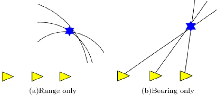
Environment modeling depends both on the complexity of the environment and on the limitations of the sensing modality. Two common examples are sonar and vision. Sonar sensors typically produce accurate range measure-ments but often have large beam-width and side-lobes mak-ing the bearmak-ing estimate unusable [33]. Measurements from a single camera, on the other hand, provide bearing infor-mation without an accurate indication of range.(a)Range only (b)Bearing only Fig. 5. Partial observation. Some sensing modalities cannot directly observe a landmark location and require observations from multiple vantage points.
SLAM with range-only sensors [34], [35] and bearing-only sensors [13], [3] show that a single measurement is insufficient to constrain a landmark location. Rather it must be observed from multiple vantage points as shown in Figure 5. More precisely, a single measurement gen-erates a non-Gaussian distribution over landmark loca-tion, and multiple measurements are needed to obtain a (nearly) Gaussian estimate. Generalised distributions, such as mixture models, permit immediate, non-delayed landmark tracking [46]. One way to obtain a Gaussian landmark estimate is to delay initialisation and instead ac-cumulate raw measurement data. To permit consistent de-layed fusion, it is necessary to record the vehicle pose for each deferred measurement. Thus, the SLAM state is aug-mented with recorded pose estimates
xk= [xTvk,xTvk−1, . . . ,xTvk−n,mT]T (15) and the corresponding measurements are stored in an aux-iliary list{zk, . . . ,zk−n}. Once sufficient information over a periodnhas been collected, a landmark is initialised by a batch update. Recorded poses that do not have any other associated measurements are then simply removed from the state.
Delayed fusion addresses far more than just partial ob-servability. It is a general concept for increasing robustness
by accumulating information and permitting delayed deci-sion making. Given an accumulated data set, an improved estimate can be obtained by performing a batch update, such as bundle-adjustment [13] or iterated fixed-interval smoothing, which dramatically reduces linearisation errors. Deferred data also facilitates batch validation gating, and so aids reliable data association.
B. Non-Geometric Landmarks
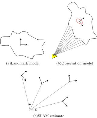
While EKF-SLAM is usually applied to geometric land-marks (often misnamed ‘point landland-marks’), the simple ex-pedient of attaching a coordinate frame to an arbitrary object allows the same methods to be applied to much more general landmark descriptions. A recent contribu-tion by Nietoet al. [42] shows that landmarks of arbitrary shape may be dealt with by using EKF-SLAM to reconcile landmark locations separately from the estimation of shape parameters.
(a)Landmark model (b)Observation model
(c)SLAM estimate
Fig. 6. SLAM with arbitrary shaped landmarks. Aligning a shape model with sensed data produces a suitable observation model for SLAM.
A landmark is described by a shape model which has an embedded coordinate frame defining the landmark ori-gin as shown in Figure 6(a). This model is auxiliary to the SLAM process, and may have any representation that permits data alignment (e.g., a grid). When the robot ob-serves the landmark, the shape model is aligned with the measurement data as shown in Figure 6(b). Assuming this alignment is approximately Gaussian, the vehicle-centric estimate of the model coordinate frame is an observation suitable for an EKF-SLAM update, where the map is com-posed of landmark frame locations as in Figure 6(c).
C. 3-D SLAM
Implementing SLAM in 3-D is, in principle, a straight-forward extension of the 2-D case. However, it involves significant added complexity due to the more general vehi-cle motion model and, most importantly, greatly increased sensing and feature modeling complexity.
There exist three essential forms of 3-D SLAM. The first is simply 2-D SLAM with additional map building capa-bilities in the third dimension. For example, horizontal laser-based SLAM with a second orthogonal laser mapping vertical slices [48], [37]. This approach is appropriate when the vehicle motion is confined to a plane. The second form is a direct extension of 2-D SLAM to 3-D, with the extrac-tion of discrete landmarks and joint estimaextrac-tion of the map and vehicle pose. This has been implemented with monoc-ular vision sensing by Davisonet al. [12], and permits full six degree-of-freedom motion. The third form involves an entirely different SLAM formulation, where the joint state is composed of a history of past vehicle poses [18], [41]. At each pose, the vehicle obtains a 3-D scan of the environ-ment and the pose estimates are aligned by correlating the scans.
D. Trajectory-Oriented SLAM
The standard SLAM formulation, as described in Part I of this tutorial, defines the estimated state as the vehicle pose and a list of observed landmarks
xk= [xTvk,mT]T. (16) An alternative formulation of the SLAM problem that has gained recent popularity is to estimate the vehicle trajec-tory instead,
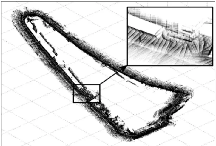
xk = [xTvk,xTvk−1, . . . ,xTv1]T. (17) This formulation is particularly suited to environments where discrete identifiable landmarks are not easily dis-cerned and direct alignment of sensed data is simpler or more reliable. Notice that the map is no longer part of the state to be estimated but rather forms an auxiliary data set. Indeed, this formulation of the SLAM problem has no explicit map, rather each pose estimate has an associated scan of sensed data, and these are aligned to form a global map. Figure 7 shows an example of this approach from [41].
The FastSLAM algorithm may also be considered as an example of trajectory estimation, with each particle defin-ing a particular trajectory hypothesis. Several recent Fast-SLAM hybrids use pose-aligned scans or grids in place of a landmark map [26], [16], [22]. Another variation of trajectory-based SLAM has developed from topologi-cal mapping [36], where poses are connected in a graph-ical network rather than a joint state vector. This frame-work, known as consistent pose estimation (CPE) [25], [31], is a promising alternative to state-space SLAM and is capable of producing large-scale maps. The advent of
Fig. 7. Trajectory-based SLAM. Scans taken at each pose are aligned according to their pose estimate to form a global map. Picture cour-tesy of [41].
sparse information form SLAM has led to a third type of trajectory-based SLAM [14], [20], [41], with sparse estima-tion of Equaestima-tion 17.
While trajectory SLAM has many positive characteris-tics, these come with caveats. Most importantly, its state-space grows unbounded with time, as does the quantity of stored measurement data. For very long-term SLAM it will eventually become necessary to coalesce data into a format similar to the traditional SLAM map to bound storage costs.
E. Embedded Auxiliary Information
Trajectory-based SLAM lends itself to representing spa-tially located information. Besides scan data for mapping, it is possible to associate auxiliary information with each pose; soil salinity, humidity, temperature, or terrain char-acteristics, for example. The associated information may be used to assist mapping, to aid data association, or for purposes unrelated to the mapping task, such as path plan-ning or data gathering.
This concept of embedding auxiliary data is more dif-ficult to incorporate within the traditional SLAM frame-work. The SLAM state is composed of discrete landmark locations and is ill suited to the task of representing dense spatial information. Nietoet al. [43] have devised a method called DenseSLAM to permit such an embedding. As the robot moves through the environment, auxiliary data is stored in a suitable data-structure, such as an occupancy grid, and the region represented by each grid-cell is de-termined by a set of local landmarks in the SLAM map. As the map evolves, and the landmarks move, the locality of the grid region is shifted and warped accordingly. The result is an ability to consistently maintain spatial local-ity of dense auxiliary information using the sparse SLAM landmark estimates.
F. Dynamic Environments
Real world environments are not static. They contain moving objects, such as people, and temporary structures
that appear static for a while but are later moved, such as chairs and parked cars. In dynamic environments, a SLAM algorithm must somehow manage moving objects. It can detect and ignore them; it can track them as moving landmarks; but it must not add a moving object to the map and assume it is stationary.
The conventional SLAM solution is highly redundant. Landmarks can be removed from the map without loss of consistency, and it is often possible to remove large num-bers of landmarks with little change in convergence rate [15]. This property has been exploited to maintain a con-temporaneous map by removing landmarks that have be-come obsolete due to changes in the environment [2, Sec-tion 5.1]. To explicitly manage moving objects, H¨ahnelet al. [27] implement an auxiliary identification routine, and then remove the dynamic information from a data scan before sending it to their SLAM algorithm. Conversely, Wang et al. [53] add moving objects to their estimated state, and provide models for tracking both stationary and dynamic targets. Simultaneous estimation of moving and stationary landmarks is very costly due to the added pre-dictive model. For this reason, the solution implemented in [53] first involves a stationary SLAM update followed by separate tracking of moving targets.
V. SLAM: Where To Next?
The SLAM method provides a solution to the key com-petency of mapping and localisation for any autonomous robot. The past decade in particular has seen substantial progress in our understanding of the SLAM problem and in the development of efficient, consistent and robust SLAM algorithms. The standard state-space approach to SLAM is now well understood and the main issues in representa-tion, computation and association appear to be resolved. The information-form of the SLAM problem has significant unexplored potential in large-scale mapping, problems in-volving many vehicles, and potentially in mixed environ-ments with sensor networks and dynamic landmarks. The delayed data fusion concept complements batch association and iterative smoothing to improve estimation quality and robustness. Appearance and pose-based SLAM methods offer a radically new paradigm for mapping and location estimation without the need for strong geometric landmark descriptions. These methods are opening up new directions and making links back to fundamental principles in robot perception.
The key challenges for SLAM are in larger and more persuasive implementations and demonstrations. While progress has been substantial, the scale and structure of many environments is limited. The challenge now is to demonstrate SLAM solutions to large problems where ro-botics can truly contribute: driving hundreds of kilometers under a forest canopy or mapping a whole city without recourse to GPS, and to demonstrate true autonomous lo-calisation and mapping of structures such as the Barrier Reef or the surface of Mars. SLAM has brought these pos-sibilities closer.
References
[1] S. Argamon-Engelson. Using image signatures for place recog-nition. Pattern Recognition Letters, 19:941–951, 1998.
[2] T. Bailey. Mobile Robot Localisation and Mapping in Exten-sive Outdoor Environments. PhD thesis, University of Sydney, Australian Centre for Field Robotics, 2002.
[3] T. Bailey. Constrained initialisation for bearing-only SLAM. In IEEE International Conference on Robotics and Automation, 2003.
[4] T. Bailey, J. Nieto, J. Guivant, M. Stevens, and E. Nebot. Con-sistency of the EKF-SLAM algorithm. InIEEE/RSJ Interna-tional Conference on Intelligent Robots and Systems, 2006. [5] Y. Bar-Shalom and T.E. Fortmann. Tracking and Data
Associ-ation. Academic Press, 1988.
[6] S.S. Blackman and R. Popoli. Design and Analysis of Modern Tracking Systems. Artech House Radar Library, 1999.
[7] M. Bosse, P. Newman, J. Leonard, M. Soika, W. Feiten, and S. Teller. An Atlas framework for scalable mapping. In IEEE International Conference on Robotics and Automation, pages 1899–1906, 2003.
[8] M. Bosse, P. Newman, J. Leonard, and S. Teller. Simultaneous localization and map building in large-scale cyclic environments using the Atlas framework. International Journal of Robotics Research, 23(12):1113–1140, 2004.
[9] K.S. Chong and L. Kleeman. Feature-based mapping in real, large scale environments using an ultrasonic array.International Journal Robotics Research, 18(1):3–19, 1999.
[10] I.J. Cox and J.J. Leonard. Modeling a dynamic environment using a bayesian multiple hypothesis approach. Artificial Intel-ligence, 66(2):311–344, 1994.
[11] M. Csorba. Simultaneous Localisation and Map Building. PhD thesis, University of Oxford, Department of Engineering Science, 1997.
[12] A.J. Davison, Y.G. Cid, and N. Kita. Real-time 3D SLAM with wide-angle vision. InIFAC/EURON Symposium on Intelligent Autonomous Vehicles, 2004.
[13] M. Deans and M. Hebert. Experimental comparison of tech-niques for localization and mapping using a bearing-only sensor. InInternational Symposium on Experimental Robotics, 2000. [14] F. Dellaert. Square root SAM: Simultaneous location and
map-ping via square root information smoothing. InRobotics: Sci-ence and Systems, 2005.
[15] G. Dissanayake, H. Durrant-Whyte, and T. Bailey. A compu-tationally efficient solution to the simultaneous localisation and map building (SLAM) problem. InIEEE International Confer-ence on Robotics and Automation, volume 2, pages 1009–1014, 2000.
[16] A.I. Eliazar and R. Parr. DP-SLAM 2.0. InIEEE Interna-tional Conference on Robotics and Automation, pages 1314– 1320, 2004.
[17] C. Estrada, J. Neira, and J.D. Tard´os. Hierarchical SLAM: Real-time accurate mapping of large environments. IEEE Transac-tions on Robotics, 21(4):588–596, 2005.
[18] R. Eustice, H. Singh, J. Leonard, M. Walter, and R. Ballard. Visually navigating the RMS Titanic with SLAM information filters. InRobotics: Science and Systems, 2005.
[19] R. Eustice, M. Walter, and J. Leonard. Sparse extended infor-mation filters: Insights into sparsification. InIEEE/RSJ Inter-national Conference on Intelligent Robots and Systems, pages 3281–3288, 2005.
[20] R.M. Eustice, H. Singh, and J.J. Leonard. Exactly sparse delayed-state filters. InIEEE International Conference on Ro-botics and Automation, pages 2417–2424, 2005.
[21] J. Folkesson and H. I. Christensen. Graphical SLAM - a self-correcting map. InIEEE International Conference on Robotics and Automation, pages 791–798, 2004.
[22] G. Grisetti, C. Stachniss, and W. Burgard. Improving grid-based SLAM with Rao-Blackwellized particle filters by adaptive proposals and selective resampling. InIEEE International Con-ference on Robotics and Automation, pages 667–672, 2005. [23] J. Guivant and E. Nebot. Optimization of the simultaneous
localization and map building algorithm for real time imple-mentation. IEEE Transactions on Robotics and Automation, 17(3):242–257, 2001.
[24] J. Guivant and E. Nebot. Improving computational and mem-ory requirements of simultaneous localization and map building
algorithms. InIEEE International Conference on Robotics and Automation, pages 2731–2736, 2002.
[25] J.S. Gutmann and K. Konolige. Incremental mapping of large cyclic environments. In IEEE International Symposium on Computational Intelligence in Robotics and Automation, pages 318–325, 1999.
[26] D. H¨ahnel, W. Burgard, D. Fox, and S. Thrun. An efficient Fast-SLAM algorithm for generating maps of large-scale cyclic envi-ronments from raw laser range measurements. InIEEE/RSJ In-ternational Conference on Intelligent Robots and Systems, pages 206–211, 2003.
[27] D. H¨ahnel, R. Triebel, W. Burgard, and S. Thrun. Map building with mobile robots in dynamic environments. InIEEE Inter-national Conference on Robotics and Automation, pages 1557– 1563, 2003.
[28] S.J. Julier and J.K. Uhlmann. A non-divergent estimation al-gorithm in the presence of unknown correlations. InAmerican Control Conference, volume 4, pages 2369–2373, 1997.
[29] S.J. Julier and J.K. Uhlmann. Using multiple SLAM algorithms. In IEEE/RSJ International Conference on Intelligent Robots and Systems, pages 200–205, 2003.
[30] J. Knight, A. Davison, and I. Reid. Towards constant time SLAM using postponement. InIEEE/RSJ International Con-ference on Intelligent Robots and Systems, pages 405–413, 2001. [31] K. Konolige. Large-scale map-making. InNational Conference
on AI (AAAI), pages 457–463, 2004.
[32] J. Leonard and P. Newman. Consistent, convergent, and constant-time SLAM. InInternational Joint Conference on Ar-tificial Intelligence, 2003.
[33] J.J. Leonard and H.F. Durrant-Whyte. Directed Sonar Sens-ing for Mobile Robot Navigation. Kluwer Academic Publishers, 1992.
[34] J.J. Leonard and R.J. Rikoski. Incorporation of delayed decision making into stochastic mapping. InInternational Symposium On Experimental Robotics, 2000.
[35] J.J. Leonard, R.J. Rikoski, P.M. Newman, and M.C. Bosse. Mapping partially observable features from multiple uncertain vantage points. International Journal of Robotics Research, 21(10–11):943–975, 2002.
[36] F. Lu and E. Milios. Globally consistent range scan alignment for environment mapping.Autonomous Robots, 4:333–349, 1997. [37] I. Mahon and S. Williams. Three-dimensional robotic mapping. InAustralasian Conference on Robotics and Automation, 2003. [38] M. Montemerlo and S. Thrun. Simultaneous localization and mapping with unknown data association using FastSLAM. In IEEE International Conference on Robotics and Automation, pages 1985–1991, 2003.
[39] J. Neira and J.D. Tard´os. Data association in stochastic map-ping using the joint compatibility test. IEEE Transactions on Robotics and Automation, 17(6):890–897, 2001.
[40] J. Neira, J.D. Tard´os, and J.A. Castellanos. Linear time vehi-cle relocation in SLAM. InIEEE International Conference on Robotics and Automation, 2003.
[41] P. Newman, D. Cole, and K. Ho. Outdoor SLAM using visual appearance and laser ranging. InIEEE International Conference on Robotics and Automation, 2006.
[42] J. Nieto, T. Bailey, and E. Nebot. Scan-SLAM: Combining EKF-SLAM and scan correlation. In International Conference on Field and Service Robotics, 2005.
[43] J. Nieto, J. Guivant, and E. Nebot. The hybrid metric maps (HYMMs): A novel map representation for DenseSLAM. In IEEE International Conference on Robotics and Automation, pages 391–396, 2004.
[44] M.A. Paskin. Thin junction tree filters for simultaneous local-ization and mapping. Technical report, University of California, Computer Science Division, 2002.
[45] Y. Rubner, C. Tomasi, and L.J. Guibas. A metric for distrib-utions with applications to image databases. InIEEE Interna-tional Conference on Computer Vision, 1998.
[46] J. Sol`a, A. Monin, M. Devy, and T. Lemaire. Undelayed ini-tialization in bearing only SLAM. InIEEE/RSJ International Conference on Intelligent Robots and Systems, pages 2751–2756, 2005.
[47] J.D. Tard´os, J. Neira, P.M. Newman, and J.J. Leonard. Robust mapping and localization in indoor environments using sonar data. International Journal of Robotics Research, 21(4):311– 330, 2002.
mobile robot mapping with applications to multi-robot and 3D mapping. InInternational Conference on Robotics and Automa-tion, pages 321–328, 2000.
[49] S. Thrun, D. Koller, Z. Ghahmarani, H. Durrant-Whyte, and A. Ng. Simultaneous localization and mapping with sparse ex-tended information filters: Theory and initial results. Technical report, Carnegie Mellon University, 2002.
[50] S. Thrun, Y. Liu, D. Koller, A. Ng, and H. Durrant-Whyte. Simultaneous localisation and mapping with sparse extended in-formation filters. International Journal of Robotics Research, 23(7–8):693–716, 2004.
[51] I. Ulrich and I. Nourbakhsh. Appearance-based place recognition for topological localization. In IEEE International Conference on Robotics and Automation, pages 1023–1029, 2000.
[52] M. Walter, R. Eustice, and J. Leonard. A provably consistent method for imposing sparsity in feature-based SLAM informa-tion filters. In International Symposium of Robotics Research, 2005.
[53] C.C. Wang, C. Thorpe, and S. Thrun. On-line simultaneous localisation and mapping with detection and tracking of mov-ing objects. InIEEE International Conference on Robotics and Automation, pages 2918–2924, 2003.
[54] Z. Wang, S. Huang, and G. Dissanayake. Decoupling localiza-tion and mapping in SLAM using compact relative maps. In IEEE/RSJ International Conference on Intelligent Robots and Systems, 2005.
[55] Z. Wang, S. Huang, and G. Dissanayake. Implementation is-sues and experimental evaluation of D-SLAM. InInternational Conference on Field and Service Robotics, 2005.
[56] S.B. Williams.Efficient Solutions to Autonomous Mapping and Navigation Problems. PhD thesis, University of Sydney, Aus-tralian Centre for Field Robotics, 2001.