Chen, Q., Liu, Y., Fioranelli, F. , Ritchie, M., Tan, B. and Chetty, K. (2019)
DopNet: A Deep Convolution Neural Network to recognize armed and
unarmed human targets.
IEEE Sensors Journal
, 19(11), pp. 4160-4172.
(doi:10.1109/JSEN.2019.2895538)
There may be differences between this version and the published version.
You are advised to consult the publisher’s version if you wish to cite from
it.
http://eprints.gla.ac.uk/177575/
Deposited on 10 January 2019
Enlighten – Research publications by members of the University of
Glasgow
DopNet: A Deep Convolution Neural Network to
Recognize Armed and Unarmed Human Targets
Qingchao Chen,
Student Member, IEEE,
Yang Liu,
Student Member, IEEE,
Francesco Fioranelli,
Member, IEEE,
Matthiew Ritchie,
Member, IEEE,
Bo Tan,
Member, IEEE,
Kevin Chetty,
Member, IEEE,
Abstract—The work presented in this paper aims to distinguish between armed or unarmed personnel using multi-static radar data and advanced Doppler processing. We propose two modi-fied Deep Convolutional Neural Networks (DCNN) termed SC-DopNet and MC-SC-DopNet for mono-static and multi-static micro-Doppler signature (µ-DS) classification. Differentiating armed and unarmed walking personnel is challenging due to the effect of aspect angle and channel diversity in real-world scenarios. In addition, DCNN easily overfits the relatively small-scale µ-DS dataset. To address these problems, the work carried out in this paper makes three key contributions:first, two effective schemes including data augmentation operation and a regularization
term are proposed to train SC-DopNet from scratch. Next,
a factor analysis of the SC-DopNet are conducted based on various operating parameters in both the processing and radar operations.Thirdly, to solve the problem of aspect angle diversity for DS classification, we design MC-DopNet for multi-static µ-DS which is embedded with two new fusion schemes termed
as Greedy Importance Reweighting (GIR) and `21-Norm. These
two schemes are based on two different strategies and have been evaluated experimentally: GIR uses a “win by sacrificing worst
case” whilst `21-Norm adopts a “win by sacrificing best case”
approach. The SC-DopNet outperforms the non-deep methods by 12.5% in average and the proposed MC-DopNet with two fusion methods outperforms the conventional binary voting by 1.2% in average. Note that we also argue and discuss how to utilize the statistics of SC-DopNet results to infer the selection of fusion strategies for MC-DopNet under different experimental scenarios.
Index Terms—DCNN, multi-static µ-DS, classification, armed personnel.
I. INTRODUCTION
Radar systems are capable of measuring Doppler directly from the frequency shift in the backscattered signal from a moving target, with respect to its original central frequency, micro-Doppler signature (µ-DS) in radar can be regarded as additional frequency modulations induced by rotating and vi-brating parts of objects, e.g. wheels of trucks, limbs movement of human targets [1–3]. In the case of people walking, the µ-DS are generated by the motion of the swinging arms, legs and torso. This phenomenon has been measured and evaluated
The manuscript was submitted for review on 23rd, Sep.2018. This work was supported by Engineering and Physical Sciences Research Council,U.K.,under grant EP/R018677/1.
Q.Chen, M.Ritchie and K.Chetty are with University College London, U.K.(emails: {qingchao.chen.13, m.ritchie, k.chetty}@ucl.ac.uk). Y.Liu is with University of Cambridge, Cambridge,U.K. (email: [email protected]). F.Fioranelli is with University of Glasgow, Glasgow, U.K. (email: [email protected]). B.Tan is with University of Coventry, Coventry, U.K. (email: [email protected].).
from a number of different radars and for a wide range of dif-ferent motions. It has been shown that movement of difdif-ferent people can be distinguished, as well as differences between men and women, people and animals [4–6]. In addition, µ-DS have been used to distinguish wind turbine blades and the blades of aircraft rotors [7]. It has also been demonstrated how µ-DS of different human target movements can help increase the situational awareness of the ambient assistant living in the healthcare context [8–14].
The focus of this article is on the training of a Deep Convolutional Neural Network (DCNN) to recognize armed and unarmed personnel using their µ-DS that have been mea-sured using a multistatic radar. µ-DSs and their applications in the context of security, warfare and healthcare have been investigated over a number of years [15–17]. The challenge of collecting the raw radar data and understanding what action is occurring can be broken down into three key steps. 1) The representation of the raw signals, 2) The features that can be extracted from them 3) The classification algorithm applied to these features. A large number of data representations, features and classifiers methods have been proposed and applied as a series of separate steps.
Due to the data being a time-frequency signal, the spectro-gram is the most common method of representing the data via a Short Time Fourier Transform (STFT). This was shown to distinguish human targets movements, e.g. walking, crawling, running etc. or to distinguish human from animals [7, 16, 17]. In addition, other time-frequency representation methods have been applied, e.g. Gabor transform, Wigner-Ville transform, Empirical Mode Decomposition based on Hilbert-Huang trans-form to extract the time-frequency representation of various human movements [18–21]. Other approaches have proposed the use of extracting empirical features, such as Radar Cross Section (RCS), Doppler bandwidth, period of motion. In addi-tion, various dimensionality reduction or de-noising methods have been investigated, like Singular Value Decomposition (SVD) method, Principle Component Analysis (PCA) and sparse representations[12, 13, 15–18].
As for the selection of classifiers, various research work related to classifiers in machine learning community have been proposed [5, 12, 13, 22]. However, these features and classifiers have not been developed and optimized in the same joint framework. This means that for different applications and conditions, the feature extraction and classifiers may need to be modified and tuned according to empirical experience, rather than using formal optimization approaches.
and computation methods such as Graphic Processing Unit (GPU), DCNNs have been proposed firstly to address the ImageNet challenge, to classify an image dataset of more than 10 million images [23]. One of the main advantages is that the feature extraction and the classifier can be jointly learned in the same framework. However, DCNN is well-known for its difficult training from scratch and normally requires large amount of data in the training stage to prevent the overfitting problem. For classification of human µ-DS, DCNN trained from scratch has been utilized and applied to distinguish hand gestures and aquatic movements using mono-static radar . However, in their approach, 80% of data is used for training and a relatively small DCNN is built to address the classification tasks [24, 25]. Recently, DCNNs have also been used for classification task of aquatic movement using the fine-tuning method, which utilized the trained DCNN network weights by ImageNet dataset so that only small part of the network weights are required to be trained [26]. For healthcare applications, this idea is further evaluated and compared with the one using auto-encoder based pre-training weights in the work of [8], which handles fine-tuning DCNNs with deep layers (e.g. VGG-Net and Inception-Net) using a small number of radar samples. In healthcare field, DCNN has also been utilized for recognizing falling based on mono-static range-Doppler signatures [27].
In this paper, we propose a modified DCNN trained from scratch called DopNet, to distinguish armed and unarmed walking human targets using the multi-static radar data. The contributions are three-folded:
1) Firstly, we propose two key novel schemes to address the over-fitting problem in training DCNN, including the radar data augmentation in the training stage and a new regularization term balancing the Mahalanobis and Euclidean distance of the network weights. We analyze the effect of various factors in the single channel DopNet (SC-DopNet) and evaluate the proposed two schemes. In addition, we compare SC-DopNet results from mono-static radar data with other handcrafted features and classifiers by experimental results.
2) Secondly, we build the multiple channel DopNet (MC-DopNet) similar to SC-DopNet and proposed two fusion methods to jointly optimize the total objective function, called Greedy Importance Reweighting (GIR) method and the`21-Norm method. Note that these two methods
are embedded in training the MC-DopNet and param-eters of the two methods can be jointly learned under the total optimization function. MC-DopNet is an end-to-end learning framework to address the classification of human µ-DS using experimental radar data.
3) Finally, we compare our proposed fusion methods to-gether with MC-DopNet to other conventional data fu-sion methods with various features and classifiers. Note that we also discuss and conclude in what scenarios the proposed two fusion methods are preferable to be utilized.
The most similar works to ours are [28] and [29] for applying DCNNs to analyze experimental multistatic radar
data, however, no proper fusion method to combine multiple DCNNs for addressing multi-static channel data has been proposed in [28] and the no detailed ablation study of net-work components are performed in [28] and [29]. Finally, no comprehensive schemes have been proposed to address the overfitting problem.
This paper is organized as follows: in section II, radar system and experiments are introduced and we propose the basic DopNet architecture and components in section III. Then we propose the SC-DopNet and MC-DopNet with two fusion schemes handling mono-static and multi-static µ-DS classification in section IV and V. Section VI is aimed at describing implementation details of the DopNet. To continue evaluating proposed methods, we present the ablation study results of SC-DopNet and analyze effect of MC-DopNet and the fusion strategies in section VII and VIII. Finally, we conclude the paper in section IX.
II. BACKGROUND
A. Radar System
The radar system used to collect the data presented in this paper is the three-node multistatic system NetRAD, which has been developed over the past years at University College London. The system is a coherent pulsed radar and operates at 2.4 GHz. The data shown in this work were collected using the following RF parameters: 0.6 µs pulse duration, 45 MHz bandwidth, linear up-chirp modulation, and 5 kHz pulse repetition frequency (PRF) to include the whole human µ-DS within the unambiguous Doppler region. Five seconds of data were recorded for each measurement in order to collect multiple periods of the average human walking gait, which is on average approximately 0.6 seconds. The transmitted power of the radar is approximately 200 mW. The antennas have 24 dBi gain and are operated with vertical polarization to effectively interact with human subjects, as the human body shape is such that the vertical dimension is more significant than the horizontal dimension. This is expected to increase the signal-to-noise of the return from the targets in comparison with horizontal polarization.
B. Experiment
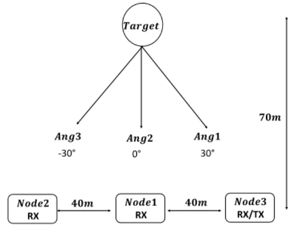
As shown in the following Fig.1, the target is walking at three different angles roughly around 30 degree, 0 degree and -30 degree, (denoted as Ang1,2,3) with respect to the radar baseline. The distance between the target position and the node 1 in the middle of the baseline is 70m. The node 3 is the Tx/Rx pulse radar part, while the other two are receivers. There are two movements in the experiment, which are walking free handed and walking while holding with both hands a metal rod which is comparable in size to a rifle. This simulated carried item was designed to cause the user to walk in the same manner as someone carrying a firle in both hands in front of them. There are three people involved into the experiments, their height are 1.87m, 1.7m and 1.75m respectively. For each walking measurement, the recorded time is 5 second and in total 180 data samples (5 second recording) are collected.
III. DOPNETARCHITECTURE
There are five main component layers in a DCNN, including the convolutional, non-linear activation, pooling, fully con-nection and the final Softmax classification layer. First these layers with their architectures and purposes will be illustrated in details in section A. In section B, operations to prevent the overfitting will be presented.
𝑻𝒂𝒓𝒈𝒆𝒕 𝑨𝒏𝒈𝟑 𝑨𝒏𝒈𝟐 𝑨𝒏𝒈𝟏 𝟕𝟎𝒎 𝑵𝒐𝒅𝒆𝟐 RX 𝑵𝒐𝒅𝒆𝟏 RX 𝑵𝒐𝒅𝒆𝟑 RX/TX 𝟒𝟎𝒎 𝟒𝟎𝒎 -30° 0° 30°
Fig. 1. Experiment scenario in the field using NetRad.
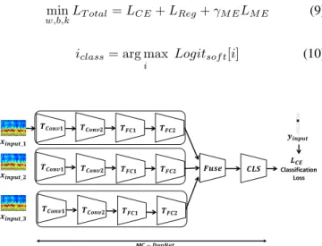
A. DopNet Component and Architecture
The network structure of DopNet is illustrated in the follow-ing Fig.2. The first two layers in DopNet are the convolution (Conv) layers, denoted as Conv1 andConv2, composed of 64 and 128 kernel filters with the size of 32x32 and 11x11 respectively. TheConvlayers are aimed to select local features of theµDsignature by convolving it with the kernels and generate activation or correlation degree maps. This can be regarded as the Conv layer outputs and these local maps will be concatenated together in a hierarchical manner [30].
To increase the model capacity of the network, We adopt the Rectified Linear Unit (ReLU) in DopNet, which is shown in Eqn.(1). Note that we apply the ReLU function following each layer output, except the output of the final layer. Additionally, we utilize the Local Response Normalization (LRN) layer developed and verified to decrease the saturation of ReLU function [30]. The idea is introduced by the lateral inhibition, which will normalize the activated map among different kernel filters. The details are shown in Eqn.(2) whereIi
w,handO i w,h are the input and output of the LRN layer activated by ith kernel at positionw, h after the ReLU layer,Ris the radius of the amount of kernels for the normalization, β can be interpreted as the polynomial parameter chosen empirically from trials and errors. This layer generalizes the network by generating competition among different kernel activations. Note that input of the LRN layer is always chosen as the output after ReLU function.
Even with the non-linear and normalization layer, represen-tation of the Conv outputs are still redundant. Therefore, the pooling layer is used as a conventional non-linear operation by only remaining the maximum among a small region of the
output activation map from Conv layers [30]. It is mostly used to simplify the network model and to extract the most useful information.
Following theConv layers are the Fully Connected (FC) layers which usually transform the local activation maps of Conv layers to the label embedding. In DopNet, we adopt a three-layer architecture with output activation number of 512, 128 and 2 respectively, directly transforming local features to the representation of semantic categories.F C layers can be regarded as a conventional linear projection operation, defined and parameterized by the weight wf c and biasbf c, but without convolutions. Due to the sparsity of the label embedding, the output of FC layersOf ccan always be added with the ReLU operation Another operation related with the F C layers is the Dropout operation, which shuts down the gradient flow and the updates of some neurons randomly for each mini-batch of data so that theF C weight matrix can be partially learned in a stochastic manner.
Lastly, the output of the final F C layer is a vector Logit ∈ RNclass×1 with the class number Nclass, each
of which indicates the probability that theµD input belongs to that class. As a model under optimization, the loss function we used is the cross-entropy (CE) function, implemented by calculating the CE between the final F C layer output and the ground-truth label, y ∈ RNclass×1, as shown in the
Eqn.(3) and (4), where Logitsof t is the output after the softmax operation andLCE is the final CE losses. Besides the Softmax cross-entropy loss, we also add a regularization term to balance the Mahalanobis and Euclidean distance for better optimization schemes. In the next section, the balancing term, together with the techniques used to prevent overfitting are introduced. ReLU(x) = max(x,0) (1) Oiw,h= I i w,h ( 1 +Pi+R/2 i−R/2(I i w,h)2)β (2) Logitsof t= exp(Logit) PNclass i=1 exp(Logit[i]) (3) LCE = Nclass X i=1
y[i]×log(Logitsof t[i]) (4)
Lreg=γf c1× kwf c=1k2+
γf c2× kwf c=2k2+
γconv1× kwc=1k2+γconv2× kwc=2k2
(5)
xaug =xwidth win,height win (6)
ky−wf c2×If c2k22=kwf c2×If cGT2−wf c2×If c2k22
= (If cGT2−If c2)Twf cT2wf c2(If cGT2−If c2)
(7)
Classification Loss 𝑻𝑪𝒐𝒏𝒗𝟏 𝒙𝒊𝒏𝒑𝒖𝒕 𝒚𝒊𝒏𝒑𝒖𝒕 𝑪𝑳𝑺 𝑳𝑪𝑬 𝑻𝑪𝒐𝒏𝒗𝟐 𝑻𝑭𝑪𝟏 𝑻𝑭𝑪𝟐 𝑺𝑪 − 𝑫𝒐𝒑𝑵𝒆𝒕 𝑻𝑪𝒐𝒏𝒗𝟏,𝟐 𝑪𝒐𝒏𝒗𝟏, 𝟐 𝑹𝒆𝑳𝑼 𝑳𝑹𝑵 𝑷𝒐𝒐𝒍 𝑻𝑭𝑪𝟏 𝑭𝒍𝒂𝒕OPT 𝑭𝑪𝟏 𝑫𝒓𝒐𝒑Out 𝑹𝒆𝑳𝑼 𝑻𝑭𝑪𝟐 𝑫𝒓𝒐𝒑 Out 𝑭𝑪𝟐 𝑬𝑴 𝑫𝒊𝒔𝒕
Fig. 2. Architecture for DopNet.
B. DopNet Operations for Overfitting Preventions
Overfitting problems are common in DCNN models, due to the fact that network parameters are biased or more discrimina-tive to the seen training samples, thus reducing generalization capabilities of the mode towards unknown testing samples. Prevention of the overfitting problem in DopNet can be solved from the following three perspectives:
1) Simplifying the network capacity: we adopt the drop-out operation of the F C2 layer and add the L2 regularization to the weight parameters of the
Conv and the F C layers, with details illustrated in Eqn.(5), where γf c1,γf c2,γconv1,γconv2 are
regu-larization weights of the L2 norm of kernel filters in F C1,F C2,Conv1,Conv2layers respectively. 2) Increasing the diversity of training data by augmentation,
i.e. by cropping the original training data into smaller patches, as showed in Fig.4. Due to the nature of the time series of the µ-DS data, we generated more training samples by cropping the data in the time domain using different stride and window sizes. As our training µ-DS data is x ∈ Rwinput×hinput, the augmented training samples can be represented as the cropped data along the time axis via different strides, as shown in Eqn.(6), where widthwin, heightwin are the window sizes
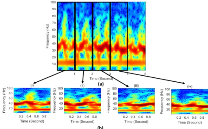
in two dimensions. This operation, if stride sizes small enough are chosen, will increase the number of training samples, give additional data diversity, and improve the robustness of the model as data generated under various conditions will be used for training. In practice, this time shifting simulates misalignment in time and small Doppler offsets for the training data, two situations that can practically happen for data collected in realistic uncontrolled scenarios. More specifically, as shown in Fig.4, an example of a target walking unarmed from angle 1, received by node 1 is illustrated. Here, in the 5-second µ-DS, four black rectangular boxes indicate four augmented data samples in the training stage. The example shown in Fig.4 useswidth winas 1 second, while theheight winchosen as 100 Hz, stride length equals to the 1 second. It seems obvious that, the augmented data samples can be generated by selecting very small stride of the moving window, which will also simulate small misalignment in realistic data.
3) Regularizing the final loss metric: we formalized the Mahalanobis distance (M-dist) and Euclidean distance (E-dist) between the ground-truth and predicted labels in DopNet. Since M-dist is aimed to maintain the discrimination capabilities while the E-dist to provide generalization, a regularization term is designed and incorporated in the DopNet by balancing the general-ization and discrimination of the network weights. Note that we balance the E-M distance only in the finalF C2 layer and denote the input, output, weights and bias in FC2 layer as If c2,Of c2,Wf c2,bf c2. If we assumed
that the ground truth label y can be transformed from the perfect inputIGT
f c2using the weightWf c2, then we
could write up the simple Euclidean loss betweenyand Wf c2×If c2as the following Eqn.(7).
In this way, we argue that this E-dist term is actually measuring the M-dist between ideal and predicted FC inputs, parameterized by weight matrixwf c2. Since
M-dist is designed to ensure the discrimination capability of the matrix, the regularized term denoted as LM E, is added to balance the E-distance and M-dist, which enforces the term wT
f c2wf c2 to be close to identity
matrix, as shown in Eqn.(8). By adjusting the balance the E and M distance, we are actually controlling the discrimination and generalization of the DCNN.
IV. SINGLE-CHANNEL(SC)-DOPNET
In this section, we introduce the single-channel (SC) Dop-Net using the components illustrated in previous sections. We introduce two phases and the relevant loss functions, including the training phase and testing phase. To sum up, the output total loss function in the training stage to optimize the DopNet is shown in Eqn.(9). Once the network parameters are stored and saved, in the test stage, given a test sample xtest, the predicted label can be calculated by the simple max operation of theLogitsof t in Eqn.(10), whereLogitsof tis the output after the Softmax operation (3) in the previous section.
min
w,b,kLT otal=LCE+LReg+γM ELM E (9)
iclass= arg max
i Logitsof t[i] (10) Classification Loss 𝑻𝑪𝒐𝒏𝒗𝟏 𝒙𝒊𝒏𝒑𝒖𝒕_𝟏 𝒚𝒊𝒏𝒑𝒖𝒕 𝑪𝑳𝑺 𝑳𝑪𝑬 𝑻𝑪𝒐𝒏𝒗𝟐 𝑻𝑭𝑪𝟏 𝑻𝑭𝑪𝟐 M𝑪 − 𝑫𝒐𝒑𝑵𝒆𝒕 𝑻𝑪𝒐𝒏𝒗𝟏 𝑻𝑪𝒐𝒏𝒗𝟐 𝑻𝑭𝑪𝟏 𝑻𝑭𝑪𝟐 𝑻𝑪𝒐𝒏𝒗𝟏 𝑻𝑪𝒐𝒏𝒗𝟐 𝑻𝑭𝑪𝟏 𝑻𝑭𝑪𝟐 𝑭𝒖𝒔𝒆 𝒙𝒊𝒏𝒑𝒖𝒕_𝟐 𝒙𝒊𝒏𝒑𝒖𝒕_𝟑
V. MULTI-CHANNEL(MC)-DOPNET
To address the diversity of aspect angle in practical sce-narios, multi-static radar can be utilized to increase the clas-sification robustness. This implies collecting simultaneous µ-DS of a particular target and activity from different, spatially distributed radar nodes. Since µ-DSs from different nodes exhibit diversed local features, it is difficult to train a single SC-DopNet local feature extractor which is sharable among signatures of all nodes. It is also a more realistic scenario that independent radar nodes would not aim to stream raw I/Q data across a network but would share a higher level classification decision into a centralised decision making system. Therefore, we choose to design multiple SC-DopNet for each radar node for MC-DopNet. The way to fuse these data into the multi-channel decision enable by MC-DopNet is introduced and discussed in this section. Two novel schemes are proposed to combine multiple channel µ-DS for recognition. The first has been formed the Greedy Importance Reweighting (GIR) method and the second is the `21-Norm method. The
MC-DopNet architecture is shown in Fig. 3. Let us assume that data fromNM C multiple channels are now available; we propose to build NM C individual SC-DopNet, where input of each SC-DopNet is data from the single channel radar. Our GIR and `21-Norm methods are proposed to fuse the outputs of
individual SC-DopNet in an end-to-end learning framework. When feed-forwarding the training data samples from mul-tiple channels through their respective SC-DopNet, the jth single channel output after Softmax function is obtained using Eqn.(3), denoted as Logitj,j ∈ [1, N
M C]. In general, we proposed two strategies to guide the fusion of multiple channel data: “win by sacrificing worst case” and “win by sacrificing best case”, guiding the design of GIR and `21-Norm method
respectively. The “win by sacrificing worst case” strategy is to increase the overall recognition rate from multiple channel data by sacrificing the performance of channels with average or bad data quality but only enhancing performance of the best single channel. The “win by sacrificing best case” strategy is to increase the overall recognition rate by degrading the channel performance with the best data quality a little but improving the performance of channel with the worst data quality.
(i) GIR Method: Our GIR method fuses multiple outputs into one final result denoted asLogitGIRbased on weighted linear combinations of individual SC-DopNet result. Note that the weights are also the parameters under DCNN training, rather than conventional binary voting schemes which combine multiple channel results under equal weights. The details are shown in Eqn.(11). To sum up, the GIR method is a greedy algorithm, because the higher weight from a given channel will be learned and assigned automatically if, and only if, its corresponding prediction output contributes more to decrease the total loss function than other channels. In addition, due to the sum of weights are forced to one, the lower weights of the other channels will be learned. To sum up, GIR method re-weights the weights of multiple channels so that the final loss function is minimized by the greatest amount.
Specifically, our GIR method uses the weighted single channel output as the fused prediction into the CE loss function
(see Eqn.(4)). Therefore, the multiple channel loss function is proposed, which is similar to Eqn.(4) except that we replace LCEbyLGIRCE , with the inputLogitGIRin Eqn.(12), where LjM EandγM Ej are thejthchannel M-dist regularization and its respective weight. LjReg is thejth channel regularization corresponding to network weights.
LogitGIR = NM C X j=1 βjLogitj, with NM C X j=1 βj = 1, βj ≥0 (11) min w,b,kL GIR T otal=L GIR CE + NM C X j=1 γjM ELjM E+LjReg (12) (ii) `21-Norm Method: Unlike the GIR method, `21-Norm
method prefers equal weights on outputs from all channels and tries to enforce similar outputs from different channels. In general, the potential advantage of `21-Norm method is
to enhance the output performance from the poor quality channel, constrained by channels with better quality results. More specifically, the `21-Norm method constrain the final
data representation of each node share the same structure. In this way, data representation from the node with bad quality is able to be compensated by the one with good quality.
Similar to the GIR method from the perspective of imple-mentation, the `21-Norm method uses a regularization term
constrained on the multiple outputsLogitj from the lastF C layer of multiple SC-DopNets. The regularization term can be shown in Eqn.(13),(14), where Logitjsof t is the output of jth channel after the Softmax operation, Logitj
sof t[i] infers the probability output that the data from jth channel belongs to the ith class. Finally, the loss function using the
`21-Norm method is shown in Eqn.(15), where LogitL21 is
the final output by averaging all single channel outputs with equal weights. LogitL21= 1 NM C NM C X j=1 Logitj (13) LL21 = Nclass X i=1 NM C X j=1 Logitjsof t[i]2 (14) min w,b,kL L21 T otal =L L21 CE + NM C X j=1 γM Ej LjM E+LjReg+γL21L L21 (15) VI. IMPLEMENTATION
First the matched filter processing between the reference and received echo signals are performed and the STFT operation is used to obtain the spectrogram. The overlapping ratio is chosen as 0.9 and the integration time for FFT is set as 0.3 seconds. Each µ-DS sample is recorded for 5 seconds and the stride for cropping the µ-DS samples in the data augmentation operation is chosen as 0.15 seconds. In addition, to increase the challenge of testing, we are also cropping the testing data into different dwell time but the stride is chosen as 0.3 seconds and the cropping starting point is chosen randomly. We argue that
this test scheme is a more realistic scenario, where we cannot guarantee where the real-time test data starts, as the radar may have been performing other tasks prior to extracting the µ-DS of a specific target at a specific time.
All DopNet layers and data operations are implemented using the Tensorflow software. The conventional Stochastic Gradient Descent (SGD) method is used for optimizing the parameters, with the momentum 0.9. The initialized learning rate for FC layers and Conv layers are chosen as 0.001 and 0.0005 respectively. The decay policy for the learning rate is the inverse decay and the decayed learning rate denoted as lrdecay is following the Eqn.(16), wherelrbase is initialized base learning rate. The batch size is chosen as 50 and training and test samples are shuffled by the Tensorflow FIFO-Queue operation. The regularization weight for the Conv and FC layers are chosen as 0.005.
lrdecay=lrbase×(1 + 0.001×epoch)−0.75 (16)
VII. RESULTS ANDABLATIONSTUDY OFSC-DOPNET
A. Raw and Augmented µ-DS
In this section, the raw µ-DS generated by STFT based on the parameters outlined in the implementation section are presented and illustrated. In addition, the data augmentation procedure and their diverse µ-DS are presented in Fig.4(b) with the raw input shown in Fig.4(a).
(a)
(b)
Fig. 4. (a)Raw Doppler signature of a target walking unarmed from angle 1, using receiver node 1;Two black bounding boxesindicate two augmented µ-DS, with window width of 1s and window height of100Hz. (b) Augmentation Results: (i), (ii), (iii) and (iv) are four augmented data examples generated from the 5-second µ-DS signature shown in Fig.4. The augmentation method and parameters are illustrated in Sec.III-B.
In Fig.5 and 6, the µ-DS related to three different angles, armed or unarmed walking gait are shown. For angle 1 and 2, the Doppler frequency related to the bulk movement is centred around 42Hz, while the one from angle 3 is around 30Hz. This is due to the relatively larger aspect angle for angle 3 than the one for angle 1 and 2. Either for armed or unarmed gaits, in general, frequency due to arms movement from angle 1 is smaller than angle 2, while the one from angle 3 is much smaller than the angle 1. The main reason might still be the different Doppler aspect angles in the bi-static radar geometry. It can be clearly seen that unarmed walking gait from Angle 1 and 2 are clearly distinguished from the armed ones by the
(a)Node1, Ang1, Walk
2 4
20 40 60 80
100 (b)Node2, Ang1, Walk
2 4
20 40 60 80
100 (c)Node3, Ang1, Walk
2 4 20 40 60 80 100
(d)Node1, Ang2, Walk
2 4
20 40 60 80
100 (e)Node2, Ang2, Walk
2 4
20 40 60 80
100 (f)Node3, Ang2, Walk
2 4 20 40 60 80 100
(g)Node1, Ang3, Walk
2 4
20 40 60 80
100 (h)Node2, Ang3, Walk
2 4
20 40 60 80
100 (i)Node3, Ang3, Walk
2 4 20 40 60 80 100
Fig. 5. Raw Doppler Signature of Walking among three angle, node and classes. All x-axis with unit of second while all y-axis with unit of Hz.
(a)Node1, Ang1, Rifle
2 4
20 40 60 80
100 (b)Node2, Ang1, Rifle
2 4
20 40 60 80
100 (c)Node3, Ang1, Rifle
2 4 20 40 60 80 100
(d)Node1, Ang2, Rifle
2 4
20 40 60 80
100 (e)Node2, Ang2, Rifle
2 4
20 40 60 80
100 (f)Node3, Ang2, Rifle
2 4 20 40 60 80 100
(g)Node1, Ang3, Rifle
2 4
20 40 60 80
100 (h)Node2, Ang3, Rifle
2 4
20 40 60 80
100 (i)Node3, Ang3, Rifle
2 4 20 40 60 80 100
Fig. 6. Raw Doppler Signature of Walking with rifle among three angle, node and classes. All x-axis with unit of second while all y-axis with unit of Hz.
signatures from 20-30Hz caused by the arms swinging. From Angle 3, shown in (h) and (i), the difference between unarmed and armed is not obvious, but some vague differences in the µ-DS map around 15Hz to 20Hz still exist.
B. Evaluating Radar Operational Parameters
In this section, we analysed the recognition rate using single channel µ-DS data with different operational parameters such as training percentage, dwell time, node geometry and all the three aspect angles. The parameter sets evaluated in the experiments are shown in the following Table I.
As shown in Fig. 7 to 10, in general, with all other variables controlled, increasing the training percentage increases the recognition rate. The reason is obvious, as it increases the
TABLE I
RADAR OPERATING PARAMETER SET UNDER EVALUATION.
Training Perc. {20%,40%,60%}
Dwell Time (Second) {1,1.5,2,2.5}
Aspect Angles (Degree) {-30,0,30}
20% 40% 60% 80 85 90 95 100 94 . 5 98 . 5 99 . 8 96 . 5 98.3 88 . 8 85 . 5 88 . 8 91. 4
Training Data Percentage
Recognition
Rates
%
Ang1 Ang2 Ang3
Fig. 7. Recognition rates for node 1, dwell time 1s, DopNet
20% 40% 60% 80 85 90 95 100 95 . 9 98 . 9 99 . 6 97 . 4 98 . 5 98 . 9 84 . 8 91 . 6 94 . 3
Training Data Percentage
Recognition
Rates
%
Ang1 Ang2 Ang3
Fig. 8. Recognition Rates for Node 1, Dwell Time 1.5s, DopNet
training data diversity and eases the classifier task by decreas-ing the test data samples. For traindecreas-ing ratio at 0.6, no matter at what dwell time, the recognition rates all achieve close to 100%. In addition, with the training ratio at 0.4, recognition rate with dwell time of 2s and 2.5s already achieves very close to 100%. However, the one with dwell time of 1s and 1.5s can only achieve 98% approximately.
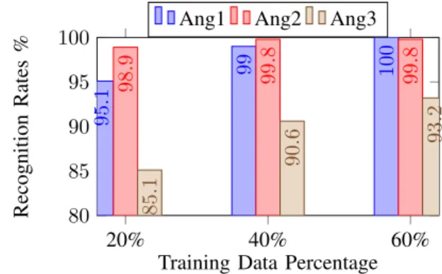
The following Fig.11 shows the averaged recognition rate among all dwell time with respect to different angles and training percentage. Among the three aspect angles, it could be found that the average recognition rate from aspect angle three is the lowest. The reason is that under movements from aspect angle 3, the bi-static angle formed by target, transmitter node 1 and the receiver node 2 is the largest that induces the lowest Doppler frequency shifts and SNR of µ-DS. These further lead to the bad discriminative quality of µ-DS from armed and unarmed motions. It can also be inferred that when trained on 20%, under all dwell time, recognition rate of angle 2 outperforms angle 1 around 2%, but with the increasing of training percentage, recognition rate of angle 1 is chasing up to equally the same as angle 2 and even outperforms angle 2 at training percentage of 0.4 and 0.6 respectively. The main reason can be observed by comparing Fig.5, 6 (a) and (d) that the Doppler frequency induced by bulk movements from angle 1 varies larger than the one from angle 2. Note that in our data augmentation steps, we are truncating the whole 5 second spectrogram into smaller parts (with shorter time duration), therefore among different augmented truncations of the dataset, augmentation from angle
20% 40% 60% 80 85 90 95 100 95 . 3 99 . 1 99 . 9 98 . 3 99 . 2 99 . 4 85 91 . 2 93. 6
Training Data Percentage
Recognition
Rates
%
Ang1 Ang2 Ang3
Fig. 9. Recognition Rates for Node 1, Dwell Time 2s, DopNet
20% 40% 60% 80 85 90 95 100 95 . 1 99 100 98 . 9 99 . 8 99 . 8 85 . 1 90 . 6 93. 2
Training Data Percentage
Recognition
Rates
%
Ang1 Ang2 Ang3
Fig. 10. Recognition Rates for Node 1, Dwell Time 2.5s, DopNet
2 will induce more variations of bulk Doppler frequency and the more of µ-DS frequency as well. This actually increases the intra-class variations among the train and test datasets. With the increasing training ratio, these intra-class variations can be eliminated as more samples related to different bulk movement Doppler shifts can be used to train the network. Finally, around training ratio of 0.6, recognition rate of angle 1 outperforms angle 2, with the potential reason that Doppler signatures induced by arms movement at unarmed scenario from angle 2 has more SNR and higher Doppler frequency shifts than angle 1, as shown in Fig.5 (a) and (d), (c) and (f). These all relate to the node 1 as the transmitter and the geometry of radar in the experiments.
Fig.12 shows the recognition rate of different angles with respect to different dwell time. Due to average on training ratio, we can deduce that for all angles, recognition rates increase with the increasing dwell time from 1s to 1.5s. However, with further increasing dwell time from 1.5s to 2.5s, only the recognition rate from angle 2 increases further and the one from angle 1 attain the similar result at dwell time of 1.5s. Note that recognition result from angle 3 drops with the further increase in dwell time. The potential reason for this may be that there are few useful features for signatures of angle 3 due to the large aspect angle.
C. Evaluating the Drop-out rate
In this section, we analyse the recognition rate with different drop-out rates via experiments. Here, we only choose the data from the following scenario: node 1, aspect angle 1,
0 0.2 0.4 0.6 0.8 Training Data Ratio
0.8 0.85 0.9 0.95 1 Recognition Rate
Angle 1 Average of All Dwell Time Angle 2 Average of All Dwell Time Angle 3 Average of All Dwell Time
Fig. 11. Recognition Rate of Different Aspect Angles respective to Training Data Ratios, Average on Dwell Time.
0.5 1 1.5 2 2.5 3
Dwell Time (Second)
0.85 0.9 0.95 1
Recognition Rate
Angle 1 Average of Percentage Angle 2 Average of Percentage Angle 3 Average of Percentage
Fig. 12. Recognition Rate of Different Aspect Angles respective to Dwell Time, Average on Training Percentage.
dwell time of 1s. The drop rate ranges from 0.2 to 0.8 in the step of 0.2 and we evaluated the respective recognition rates. According to Fig.14,when trained with 20% and 40% data, increasing the dropping rate from 0.2 to 0.8 on FC1 will increases the recognition rates first (when increasing from 0.2 to 0.4) and then decreases them (when increasing the drop-out rate from 0.4 to 0.8). This is due to the fact that the model is first overfitting the data where the model parameter number is so large as to over-parameterize the training data completely but the generalization capability of the model to the test data cannot be maintained. Increasing drop rate from 0.2 to 0.4 then ensures the network capability is relative to generalization. When the dropping rate increases further, the network parameters are relatively small to model the training data, which decreases the capability of the model and the recognition rate. In addition Fig.14 shows that when trained with 60% of the data, increasing the drop-rate from 0.2 to 0.6 continuously increase the recognition rates and then further increasing will decrease the recognition rate. The reason can be attributed to previously described scenario.
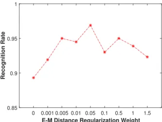
D. Evaluating E-dist and M-dist
In this section, we analyze and evaluate the regulariza-tion weight of the balancing E-M distances, by compar-ing different recognition rates based on whether M or E distance metric dominates. The experiments are conducted using node 1, angle 1, dwell time 1s with 20% training
0 0.001 0.005 0.01 0.05 0.1 0.5 1 1.5
E-M Distance Regularization Weight
0.85 0.9 0.95 1
Recognition Rate
Fig. 13. Recognition Rate of Different E-M Distance Regularization Weights.
20% 40% 60% 90 92 94 96 98 100 94 . 5 98 . 3 98 . 9 95 . 4 98 . 6 99 . 1 94 . 5 98 . 5 99. 8 94 . 5 98 . 4 99 . 3 Recognition Rates %
Drop 20% Drop 40% Drop 60% Drop 80%
Fig. 14. Angle 1, Node 1, Dwell Time 1s with different drop rate
data. As shown in Fig.13 increasing the hyper-parameter
γM E in Eqn.(9) from 0 to 1.5 based on the following set
{0,0.001,0.005,0.01,0.05,0.1,0.5,1,1.5}induces the results increasing from 89.3% to top 96.9% and then dropping to 93.3%. At first, the M-distance dominates, but this is prone to overfitting the data. Then due to the increasing of the balancing weights, the good balance between M and E distance is able to maintain both generalization and discrimination capability of the network. Increasing the balancing weights further will then drop the recognition rate again, as the model generalizes too much but lose the discrimination capability. In this scenario, we choose 0.05 as our optimal balanced hyper-parameter.
TABLE II
NODE1, DWELLTIME1S, DOPNET WITH DIFFERENTSNRS
SNR:-10 SNR:-5 SNR:5 SNR:10 Ang1 94.2% 95.5% 95.8% 96.0% Ang2 96.1% 96.5% 96.9% 96.8% Ang3 83.6% 84.3% 84.9% 85.3%
E. Evaluating the SNRs and Memory Usage
As shown in Table II, recognition rates based on different SNR levels are shown. It could be observed that increasing the SNR from -10 to 5 dB increases the recognition rate by 2% while recognition rate stays stably the same if we further increase the SNR from 5dB to 10dB.
In addition, we discuss memory usage of the network. In the practical scenario, the dataset can be trained on the server or computer cluster therefore only the weights of the network need to be carried onto the site. We also report the memory usage of the network weights in our single channel DopNet as 44MB. For the all angles in test of 216/648 test samples (each is a 0.3second µ-DS), the processing time of each testing stage is 0.17/0.52 second in average. The processing time in the test stage is roughly linearly proportional to the number of test data and the ratio is 0.085 second per 100 samples. To sum up, the SC-DopNet is big as 44MB and can predict one test sample in 850 µs.
F. Comparison with Empirical Features and Classifiers
In Table III, we compared results of DopNet with other features extraction methods(including the state-of-the-art SVD and centroid features [7, 15, 16]) and classification methods (including the Nave Bayes (NB) classifier, the Discriminative Analysis (DA) method and Classification Tree (CT) method [31]). The experiment setting for Table III is aimed to analyze recognition performance under node 1 and each of all angles. For each experiment, we report the best recognition rates selecting different combination of features and we highlight the best recognition rates by red. With increasing of dwell time, under various classification methods, the recognition rates all increase. Obviously, angle 1 is the angle with the best recognition rate using other non-DopNet features and recognition rates of DopNet outperform 1-2% under dwell time from 1s to 2s. At dwell time of 2.5s, combination of SVD and centroid features outperforms DopNet by 0.5%. However, for experiment in angle 2, DopNet outperforms other methods by 10%. For experiments in angle 3, DopNet outperforms others by around 7% with 1s and 1.5s dwell time but achieves only 2-3% better than the other methods in dwell time of 2s and 2.5s.
In Table IV, we proposed a new measure where all three angles from a single node are included in the dataset to recognition armed and unarmed movements. We argue that this is a more realistic scenario compared to mono-static radar recognition, as µ-DS from all aspect angles can po-tentially be the dataset. It can be observed that under this more complicated task, recognition rates using non-DopNet features and classification methods drop around 5% for node 1 compared with the average in Table III, however, DopNet results achieve similar performance, achieving averaged 93.5% under all dwell-time settings. For node 2, DopNet still outper-forms others by approximately 10%. For the most difficult result for node 3, it seems that adding all-angle signatures increases the DopNets performances outperforming 15% than the other features and achieving around 92.3% for all dwell-time settings.
To sum up, compared with non-deep feature and classifier, DopNet achieved in average 92.7%, outperforming the second best feature and classifier (DA method) 4% when evaluating for single angle in node 1 scenario. When mixing up µ-DS of all angles, DopNet achieved the most robust results, in average 91.0%, outperforming the second best around 12.6%. This is mainly due to DopNet’s large model capacity when handling
complex classification tasks, for example the classification of all-angle scenario. From another perspective, since we do not change the hyper-parameters, it is beneficial to train DopNet using larger number of training data.
VIII. RESULTS, DISCUSSION ANDABLATIONSTUDY OF
MC-DOPNET
In the previous section, we analyzed detailed DopNet pa-rameters using the single channel data. In this section, we discussed the feasibility of extending the SC-DopNet to MC-DopNet to optimize the processing from multiple multistatic radar nodes. In addition, we evaluated our proposed two methods, namely GIR and `21-Norm method, by comparing
with the conventional binary voting schemes. Specifically, the recognition results are shown in Tables V, VI, VII respectively generated respectively by Binary Voting (BV) method, GIR method and the `21-Norm method. In these three tables, the
final fusion recognition rates, their respective recognition rate using the single channel prediction output (but trained by fusing all multiple channel data) and the learned weights (for GIR method only) are shown and compared. Additionally, in Fig.5 and 6, we show the raw µ-DS for all the nodes, angle and classes to analyze its corresponding recognition rate.
A. Analysis of the results based on different node-angle com-binations from multiple channels
In this section, the aim is to compare MC-DopNet results using our proposed GIR and `21-Norm with the one using
conventional binary voting (BV) [7]. In general, the BV method accepts the decision result if at least two out of three nodes’ results are the same, given that our problem is the binary classification. All experiments are conducted using 30 trials with randomly selected training and test samples. To ensure fair testing, experimental settings are the same for all three methods: dwell time at 1s, training with 20%, with the same augmentation scheme and SC-DopNet architecture, as introduced in previous sections.
Although results in Table V,VI and VII are trained based on fusing multiple channel data, we argue that recognition result based on certain node-angle combinations is an indirect way to understand performance and mechanism of fusion methods.Therefore, we propose to use recognition rates by BV methods as baseline to measure the performance of certain node-angle combination. The main reason is that the total loss function of BV method is simply the sum of the loss functions from three networks with equal weights. There are three main findings by observing the Table V and corresponding signatures in Fig.5 and 6.
1) Finding 1:It can be figured out in the first three columns in Table V and VII that, for all angles independent of the fusing method, recognition rates from Node 1 outperform Node 2 and 3 and those from Node 3 outperform Node 2. This matches the higher SNR µ-DS and more discriminative features of Node 1 than Node 3 and the one of Node 3 than Node 2. The main reason is the larger bi-static angle formed by receiver Node 2
TABLE III
NODE1, DWELLTIME: 1S-2.5S, 20%TRAINING, MONO-DATAONLY, PERCENTAGE IN(%)
Features Best Combined SVD and Centroid Features DopNet Dwell Time 1s 1.5s 2s 2.5s 1s 1.5s 2s 2.5s
Classifier NB DA CT NB DA CT NB DA CT NB DA CT Soft-max and Max A1,N1 93.1 93.0 88.2 93.5 93.9 91.9 94.5 94.7 94.2 96.1 95.096.2 94.5 95.9 95.3 95.1 A2,N1 83.7 83.8 78.6 78.3 84.2 80.2 84.2 83.9 83.1 84.5 84.7 80.5 96.5 97.4 98.3 98.9
A3,N1 76.7 75.4 69.2 79.6 79.5 74.7 84.3 82.0 78.8 84.1 83.0 76.7 85.5 84.8 85.0 85.1
Average 84.5 84.1 78.7 83.8 85.9 82.3 87.7 86.9 85.4 88.2 87.6 84.5 92.2 92.7 92.8 93.0
TABLE IV
ALLNODES ANDALLANGLES IN, DWELLTIME: 1S-2.5S, 20%TRAINING, MONO-DATAONLY, PERCENTAGE IN(%)
Features Best Combined SVD and Centroid Features DopNet Dwell Time 1s 1.5s 2s 2.5s 1s 1.5s 2s 2.5s
Classifier NB DA CT NB DA CT NB DA CT NB DA CT Soft-max and Max N1 80.4 80.4 77.4 81.4 81.7 79.4 82.3 81.9 81.2 83.2 82.6 82.6 92.6 93.0 93.7 93.5 N2 70.9 70.0 64.7 73.1 72.8 66.9 73.1 72.7 68.9 73.0 72.8 68.3 80.2 83.6 83.2 83.9 N3 74.2 74.2 72.3 76.2 75.6 75.0 77.5 77.3 77.3 77.9 77.8 77.7 90.1 92.7 93.5 92.9 Average 75.2 74.9 71.5 76.9 77.5 76.7 77.6 77.3 75.8 78.0 77.7 76.2 87.6 89.8 90.1 90.1
TABLE V
DWELLTIME1S, DOPNET, 20%TRAINING, BV METHOD, AINDICATES
ANGLE IN THE FOLLOWING TWO FIGURES.
Node 1 Node 2 Node 3 BV Accuracy Accuracy Accuracy Accuracy
(weight) (weight) (weight)
A1 95.7 (0.333) 65.0 (0.333) 87.1 (0.333) 96.1 A2 96.5 (0.333) 77.3 (0.333) 93.5 (0.333) 99.0 A3 85.3 (0.333) 70.8 (0.333) 81.8 (0.333) 91.7
TABLE VI
DWELLTIME1S, 20%TRAINING, GIR METHOD.
Node 1 Node 2 Node 3 BV Accuracy Accuracy Accuracy Accuracy
(weight) (weight) (weight)
A1 97.3 (0.421) 50.7 (0.289) 49.3 (0.289) 98.2 A2 98.2 (0.434) 50.1 (0.283) 51.2 (0.283) 98.9 A3 88.8 (0.462) 51.7 (0.269) 48.3 (0.269) 89.5
and transmitter Node 3, which decreases both SNR and the frequency shifts related with motions from Node 3. 2) Finding 2:From Table V, all recognition results from A2 and A1 outperforms A3, no matter which node is se-lected. This matches with our observation of the (a) and (b) in Fig.5 and Fig.6, where better data quality (SNR) from angle 1 and angle 2 induce better discriminative quality than the angle 3, no matter from which node. 3) Finding 3: The recognition results from A2 always
outperform the A1. The main reason is that the Doppler frequency induced by bulk movements from angle 1 varies larger than the one from angle 2. This can be observed by comparing (a) and (d), (b) and (e) of Fig.5 and Fig.6 respectively. More detailed discussions can be found in previous section VII-B.
In Table VI, when the GIR method is utilized, it can only be found that recognition rate from node 1 outperforms the others, but the one of node 2 and node 3 are basically the same. Specifically, from the first column in Table V, VI and
TABLE VII
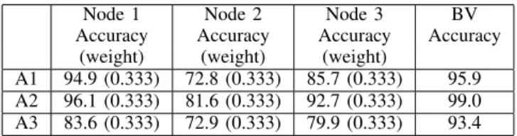
DWELLTIME1S, DOPNET, 20%TRAINING,`21-NORMMETHOD.
Node 1 Node 2 Node 3 BV Accuracy Accuracy Accuracy Accuracy
(weight) (weight) (weight)
A1 94.9 (0.333) 72.8 (0.333) 85.7 (0.333) 95.9 A2 96.1 (0.333) 81.6 (0.333) 92.7 (0.333) 99.0 A3 83.6 (0.333) 72.9 (0.333) 79.9 (0.333) 93.4
VII, it can be figured out that node 1 recognition results from whatever angle using GIR method outperforms`21-Norm and
BV method for around 3%. In addition, from the second and third columns, recognition rates of GIR from node 2 and 3 drop significantly compared to other two methods. The reason is the greedy nature of GIR which is aimed to increase the weights from the best quality channel node 1 and decrease the ones from other channels in the fusing mechanism. This explanation can also be verified by the extremely unbalanced weights, found in Table VI, where weight from node 1 with all angles are larger than other nodes; meanwhile, weights of node 2 and 3 are approximately the same.
It can be found that for all angles, `21-Norm method
outperforms the BV method from node 2 data but performs worse than BV method from node 1 and 3. Specifically, comparing the first row in Table V and VII, with the use of
`21-Norm method, the recognition rate from Node 2 (with the
worst data quality) increases from 65% (using BV method) to 72.8% (using`21-Norm method), the recognition rate from
node 1 and 3 decreases from 95.7% (using BV method) to 94.9% (using`21-Norm) and from 87.1% (using BV method)
to 85.7% (using`21-Norm). Similar pattern can also be found
from observations of other rows in Table 5 V and VII. This phenomenon can be interpreted by the nature of `21-Norm,
where similar prediction outputs are enforced among multiple channels. From other words, to enhance the performance of node 2 with the worst data quality, the `21-Norm sacrifices
TABLE VIII
NODE1, DWELLTIME: 1S-2.5S, 20%TRAINING, MONO-DATAONLY, PERCENTAGE IN(%)
Features Best Combined SVD and Centroid Features DopNet Dwell Time 1s 1.5s 2s 2.5s 1s 1.5s 2s 2.5s
Classifier NB DA CT NB DA CT NB DA CT NB DA CT Soft-max and Max A1,N1 93.1 93.0 88.2 93.5 93.9 91.9 94.5 94.7 94.2 96.1 95.0 96.2 94.5 95.9 95.3 95.1 A2,N1 83.7 83.8 78.6 78.3 84.2 80.2 84.2 83.9 83.1 84.5 84.7 80.5 96.5 97.4 98.3 98.9 A3,N1 76.7 75.4 69.2 79.6 79.5 74.7 84.3 82.0 78.8 84.1 83.0 76.7 85.5 84.8 85.0 85.1
TABLE IX
COMPARISON OFDOPNETRESULTS ANDOTHERFEATUREEXTRACTIONMETHOD ANDCLASSIFIERS. FOR FAIR COMPARISON,WE SELECT THE BEST THRESHOLDING VOTING SCHEME AND FEATURES ARE THE BEST COMBINATIONS REPORTED IN THE PAPER[17]; PERCENTAGE IN(%).
Feat Best Combined SVD and Centroid Features DopNet DopNet DT 1s 1.5s 2s 2.5s 1s 1.5s 2s 2.5s 1s 1.5s 2s 2.5s Cls NB DA CT NB DA CT NB DA CT NB DA CT Soft-max(GIR) Soft-max(`21-Norm)
A1 91.1 91.3 89.2 92.4 92.3 91.8 93.5 93.7 93.5 95.6 95.7 93.2 98.2 97.2 98.2 98.5 95.9 95.9 95.4 94.9 A2 90.8 91.9 92.0 93.4 93.5 94.8 94.2 94.7 95.9 95.7 96.9 96.6 98.9 99.6 100.0 100.0 99.0 99.0 99.0 99.4 A3 79.4 79.4 77.2 81.7 82.6 80.0 84.3 84.7 82.1 83.4 84.2 83.4 89.5 89.1 88.2 88.7 93.4 92.3 93.5 93.0 All 80.9 80.7 80.7 82.1 82.9 83.9 83.3 84.0 85.6 84.5 84.4 86.9 93.7 94.3 94.9 94.3 93.2 94.7 94.6 95.6
of single channel recognition rates but such fusion mechanism outperforms others from the total fused recognition rate.
B. Compare the fusion method using MC-DopNet
In this section, we focus on comparing the recognition results based on multi-channel data using different fusion methods. For fusion results based on angle 1, GIR method achieves the best, approaching to 98.2% in average, outper-forming the BV method (96.1%) and the `21-Norm method
(95.9%). Looking at the weights in Table VI, it seems that the greedy-like algorithm assigns the biggest weight to the node 1 (around 0.421) while assigns equally (around 0.289) to the other two. This matches our assumption and understanding of the greedy algorithm discussed before in the three findings.
For recognition based on angle 2, no matter for BV, GIR and `21-Norm exhibit similar and the best recognition result
(around 99%), due to the data having the highest SNR and discriminative features. For results based on angle 3 with the worst data quality, the `21-Norm method achieves the best
93.4% compared with BV method at 91.7% and GIR method at 89.5%. The main reason has been discussed in section V.B
TABLE X
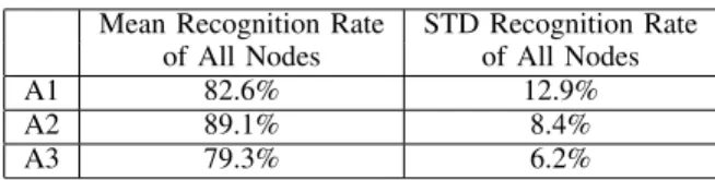
MEAN AND STANDARD DEVIATION OF RESULTS INTABLEVBYBV
METHOD.
Mean Recognition Rate STD Recognition Rate of All Nodes of All Nodes
A1 82.6% 12.9%
A2 89.1% 8.4%
A3 79.3% 6.2%
In addition, we investigate and discuss when, especially for which angle, GIR and`21-Norm should be utilized to improve
fusion results. We generate Table X by calculating the mean and STD of results using BV method (based on Table V). We argue that the mean and STD of recognition results are useful to determine the preferable method for certain angle.
It is easy to conclude from Table VI and VII that when fus-ing multi-channel results for angle 2, the three fusion methods
achieve similar result due to its originally good discriminative quality. However in Table VIII, when the mean recognition accuracy is relatively high but the standard variation is very large, like angle 1, the GIR method is more suitable for the fusion task. For the low mean accuracy and low STD scenario,
`21-Norm might achieve the best to fuse these multi-channel
data.
C. Compare MC-DopNet with other methods
In this section, we compared our results with the state-of-the-art SVD and centroid features, using the threshold voting as the fusion method in Table IX. The experiment setting is to recognize the µ-DS from a specific angle using all three multi-static nodes. It can be observed that from Angle 1 and angle 2, MC-DopNet with GIR method achieves the best, outperforming other methods by 3% to 5% depending on different dwell time. For angle 3, MC-DopNet with `21
-Norm method outperforms all other methods by 6% to 17% depending on different dwell time. For the most difficult test scheme with all angle data in, MC-DopNet based methods generally outperform 10% than others in average. The reason has been explained in the previous three findings. Note that for all features and methods, recognition rate from all angles should be lower than the best single angle but still better than the worst single angle result.
IX. CONCLUSION
Multistatic radar has been shown to address the problem of degradation of classification performance due to unfavorable aspect angles when extracting µ-DS. This paper proposed a modified DCNN, namely DopNet, for recognition of armed and unarmed personnel using µ-DS from multi-static radar data. First, two effective schemes including data augmentation and the balancing the E-dist and M-dist have been proposed, so that DopNet can be trained from scratch and relevant features and classifiers can be jointly learned in the same framework. In addition, performances of SC-DopNet and the analysis of
relevant operational parameters has been conducted. In order to exploit effectively simultaneous information from different radar channels for the MC-DopNet training, two fusion strate-gies have been proposed to embed multi-static µ-DS. We also discussed how to utilize the statistics of single channel results to infer the selection of fusion strategies. Both SC-DopNet and MC-DopNet have been evaluated by experimental data and the results have been compared with other state-of-art methods to prove its superior performances. Future work will focus on investigating the performance of methods in challenging scenarios, such as different body types, more challenging activities under classification and even running or walking with different objects carried. In addition, it is worth investigating the effect of unseen body types and objects in the training stage. Another future direction may consider more classes, for example the case of walking carrying something in one hand but not a weapon.
REFERENCES
[1] V. C. Chen, F. Li, S.-S. Ho, and H. Wechsler, “Micro-doppler effect in radar: phenomenon, model, and sim-ulation study,” IEEE Transactions on Aerospace and electronic systems, vol. 42, no. 1, pp. 2–21, 2006. [2] V. C. Chen,The micro-Doppler effect in radar. Artech
House, 2011.
[3] V. C. Chen, W. J. Miceli, and D. Tahmoush,Radar micro-Doppler signatures: processing and applications. The Institution of Engineering and Technology, 2014. [4] Y. Kim, S. Ha, and J. Kwon, “Human detection
us-ing doppler radar based on physical characteristics of targets,” IEEE Geoscience and Remote Sensing Letters, vol. 12, no. 2, pp. 289–293, 2015.
[5] Y. Kim and H. Ling, “Human activity classification based on micro-doppler signatures using a support vector machine,”IEEE Transactions on Geoscience and Remote Sensing, vol. 47, no. 5, pp. 1328–1337, 2009.
[6] R. M. Narayanan and M. Zenaldin, “Radar micro-doppler signatures of various human activities,”IET Radar, Sonar & Navigation, vol. 9, no. 9, pp. 1205–1215, 2015. [7] F. Fioranelli, M. Ritchie, A. Balleri, and H. Griffiths,
“Practical investigation of multiband mono-and bistatic radar signatures of wind turbines,”IET Radar, Sonar & Navigation, vol. 11, no. 6, pp. 909–921, 2017.
[8] M. S. Seyfio˘glu and S. Z. G¨urb¨uz, “Deep neural network initialization methods for micro-doppler classification with low training sample support,”IEEE Geoscience and Remote Sensing Letters, vol. 14, no. 12, pp. 2462–2466, 2017.
[9] B. Jokanovic, M. Amin, and B. Erol, “Multiple joint-variable domains recognition of human motion,” in
Radar Conference (RadarConf), 2017 IEEE. IEEE, 2017, pp. 0948–0952.
[10] B. Jokanovic, M. G. Amin, and F. Ahmad, “Effect of data representations on deep learning in fall detection,” in Sensor Array and Multichannel Signal Processing Workshop (SAM), 2016 IEEE. IEEE, 2016, pp. 1–5.
[11] B. Jokanovic, M. Amin, and F. Ahmad, “Radar fall mo-tion detecmo-tion using deep learning,” inRadar Conference (RadarConf), 2016 IEEE. IEEE, 2016, pp. 1–6. [12] Q. Chen, M. Ritchie, Y. Liu, K. Chetty, and K.
Wood-bridge, “Joint fall and aspect angle recognition using fine-grained micro-doppler classification,” in Radar Confer-ence (RadarConf), 2017 IEEE. IEEE, 2017, pp. 0912– 0916.
[13] Q. Chen, B. Tan, K. Chetty, and K. Woodbridge, “Ac-tivity recognition based on micro-doppler signature with in-home wi-fi,” in e-Health Networking, Applications and Services (Healthcom), 2016 IEEE 18th International Conference on. IEEE, 2016, pp. 1–6.
[14] F. Fioranelli, M. Ritchie, and H. Griffiths, “Bistatic human micro-doppler signatures for classification of in-door activities,” inRadar Conference (RadarConf), 2017 IEEE. IEEE, 2017, pp. 0610–0615.
[15] F.Fioranelli, M.Ritchie, and H.Griffiths, “Performance analysis of centroid and svd features for personnel recog-nition using multistatic micro-doppler,”IEEE Geoscience and Remote Sensing Letters, vol. 13, no. 5, pp. 725–729, May 2016.
[16] F. Fioranelli, M. Ritchie, and H. Griffiths, “Multistatic human micro-doppler classification of armed/unarmed personnel,”IET Radar, Sonar & Navigation, vol. 9, no. 7, pp. 857–865, 2015.
[17] F.Fioranelli, M.Ritchie, and H.Griffiths, “Aspect angle dependence and multistatic data fusion for micro-doppler classification of armed/unarmed personnel,” IET Radar, Sonar & Navigation, vol. 9, no. 9, pp. 1231–1239, 2015. [18] G. Li, R. Zhang, M. Ritchie, and H. Griffiths, “Sparsity-driven micro-doppler feature extraction for dynamic hand gesture recognition,” IEEE Transactions on Aerospace and Electronic Systems, 2017.
[19] D. P. Fairchild and R. M. Narayanan, “Classification of human motions using empirical mode decomposition of human micro-doppler signatures,” IET Radar, Sonar & Navigation, vol. 8, no. 5, pp. 425–434, 2014.
[20] A. Brewster and A. Balleri, “Extraction and analysis of micro-doppler signatures by the empirical mode decom-position,” inRadar Conference (RadarCon), 2015 IEEE. IEEE, 2015, pp. 0947–0951.
[21] S. Z. G¨urb¨uz, B. Erol, B. C¸ a˘glıyan, and B. Tekeli, “Operational assessment and adaptive selection of micro-doppler features,”IET Radar, Sonar & Navigation, vol. 9, no. 9, pp. 1196–1204, 2015.
[22] M. Ritchie, M. Ash, Q. Chen, and K. Chetty, “Through wall radar classification of human micro-doppler using singular value decomposition analysis,”Sensors, vol. 16, no. 9, p. 1401, 2016.
[23] K. Simonyan and A. Zisserman, “Very deep convo-lutional networks for large-scale image recognition,”
CoRR, vol. abs/1409.1556, 2014.
[24] Y. Kim and T. Moon, “Human detection and activity classification based on micro-doppler signatures using deep convolutional neural networks,” IEEE Geoscience and Remote Sensing Letters, vol. 13, no. 1, pp. 8–12, 2016.
[25] Y. Kim and B. Toomajian, “Hand gesture recognition using micro-doppler signatures with convolutional neural network,”IEEE Access, vol. 4, pp. 7125–7130, 2016. [26] Y. Kim, J. Park, and T. Moon, “Classification of
micro-doppler signatures of human aquatic activity through sim-ulation and measurement using transferred learning,” in
Radar Sensor Technology XXI, vol. 10188. International Society for Optics and Photonics, 2017, p. 101880V. [27] B. Jokanovi´c and M. Amin, “Fall detection using deep
learning in range-doppler radars,”IEEE Transactions on Aerospace and Electronic Systems, vol. 54, no. 1, pp. 180–189, 2018.
[28] Z. Chen, G. Li, F. Fioranelli, and H. Griffiths, “Personnel recognition and gait classification based on multistatic micro-doppler signatures using deep convolutional neural networks,” IEEE Geoscience and Remote Sensing Let-ters, 2018.
[29] J. S. Patel, F. Fioranelli, M. Ritchie, and H. Griffiths, “Multistatic radar classification of armed vs unarmed personnel using neural networks,”Evolving Systems, pp. 1–10, 2017.
[30] A. Krizhevsky, I. Sutskever, and G. E. Hinton, “Imagenet classification with deep convolutional neural networks,” in Advances in neural information processing systems, 2012, pp. 1097–1105.
[31] J. Friedman, T. Hastie, and R. Tibshirani, The elements of statistical learning. Springer series in statistics New York, NY, USA:, 2001, vol. 1, no. 10.