Determination of
vector error correction models
in high dimensions
by Chong Liang and Melanie Schienle
No. 124 | JANUARY 2019
Impressum
Karlsruher Institut für Technologie (KIT) Fakultät für Wirtschaftswissenschaften Institut für Volkswirtschaftslehre (ECON)
Kaiserstraße 12 76131 Karlsruhe
KIT – Die Forschungsuniversität in der Helmholtz-Gemeinschaft Working Paper Series in Economics
No. 124, January 2019 ISSN 2190-9806
Determination of Vector Error Correction Models in High
Dimensions
IChong Lianga, Melanie Schienleb,˚
aKarlsruhe Institute of Technology (KIT) bKarlsruhe Institute of Technology (KIT)
Abstract
We provide a shrinkage type methodology which allows for simultaneous model selection and estimation of vector error correction models (VECM) when the dimension is large and can increase with sample size. Model determination is treated as a joint selection problem of cointegrating rank and autoregressive lags under respective practically valid sparsity assumptions. We show consistency of the selection mechanism by the resulting Lasso-VECM estimator under very general assumptions on dimension, rank and error terms. Moreover, with computational complexity of a linear programming problem only, the procedure remains computationally tractable in high dimensions. We demonstrate the effectiveness of the proposed approach by a simulation study and an empirical application to recent CDS data after the financial crisis.
Keywords: High-dimensional time series, VECM, Cointegration rank and lag selection, Lasso, Credit Default Swap
JEL: C32, C52
1. Introduction
Complex financial systems are dynamic, high-dimensional and often contain a large number of non-stationary potentially cointegrated components. Examples include the de-gree of interdependence of corporate debt among different banks and its interplay with sovereign debt, both measured as a large system of credit default spreads (CDS), but also risk analysis for large-dimensional portfolios containing many different nonstation-ary elements such as exchange or interest rates in the presence of a limited number of applicable observations during crisis times. Generally, the standard tool to handle mul-tivariate nonstationary time-series has been the vector error correction model (VECM)
IWe are grateful to Weibiao Wu, Qiwei Yao and Rongmao Zhang for helpful discussions. We
further-more thank the editor, Oliver Linton, and three anonymous referees for constructive comments which led to substantial improvements of the paper. We acknowledge support from Deutsche Forschungsgemein-schaft through grant SCHI-1127.
˚Corresponding author. Address: Karlsruhe Institute of Technology, Department of Economics
(ECON), Chair of Econometrics and Statistics, Bl¨ucherstr. 17, 76185, Karlsruhe, Germany. Tel: +49
as introduced by Engle and Granger (1987). But even for settings with a fixed number of dimensions mildly exceeding two, existing econometric techniques for VECM often fail to provide accurate, testable and computationally tractable estimates, e.g. sequential Jo-hansen tests (JoJo-hansen, 1988, 1991) and refinements thereof such as e.g. Xiao and Phillips (1999), Hubrich, L¨utkepohl and Saikkonen (2001), Boswijk, Jansson and Nielsen (2012), Cavaliere et al. (2012). In the high-dimensional case of the examples before, however, also information criteria based techniques such as Chao and Phillips (1999) are no longer appli-cable and novel types of methods are required which need a completely different statistical analysis. Such techniques are important for understanding the explicit interplay of differ-ent market compondiffer-ents in order to judge their systemic importance and market relevance. In this paper, we provide a Lasso-type technique for consistent and numerically ef-ficient model selection when the dimension is allowed to increase with the number of observations at some polynomial rate. Model determination is treated as a joint selection problem of cointegrating rank and VAR lags. In this case, we exploit a sparse model struc-ture in the sense that from a large number of potential cointegration relations, in practice, only a small portion of them are actually prevalent for the system. In the same way, a small and fixed number of VAR lags is considered sufficient for a parsimonious model specification. Within this maximum lag range, however, our model selection technique is independent from the lag ordering detecting non-consecutive lags. We show consistency of model selection by the proposed adaptive group Lasso-VECM estimator requiring only weak moment conditions on the innovations allowing for a wide range of applications. Moreover, we also cover the case of weak dependence in the error term and obtain rank selection consistency despite the fact that least squares pre-estimates of the cointegra-tion matrix are inconsistent in this case. As a by-product, we also derive the statistical properties of the obtained Lasso-estimates for the loadings. A simulation study shows the effectiveness of the proposed techniques in finite samples treating cases of dimension up to 50 with realistic empirical sample sizes. In the empirical example, the new techniques allow us to study a joint system of 15 credit default swaps (CDS) log prices of European sovereign countries and banks - for which there has been no theoretically valid and feasible model determination technique in the literature so far.
Our work builds on the excessive literature of VECM as summarized e.g. in L¨utkepohl (2007) as well as on results for Lasso-type techniques from the standard i.i.d. setting originating from Tibshirani (1996) and Knight and Fu (2000). In particular, we employ ideas from adaptive Lasso by Zou (2006) for improved selection consistency properties by weighted penalties and use the group structure as in Yuan and Lin (2006) for group-Lasso which allows for simultaneous exclusion and inclusion of certain variables. For the high-dimensional case, consistency results for Lasso have been developed by Bickel, Ritov and Tsybakov (2009) , Zhao and Yu (2006) and in a group-Lasso case in Wei and Huang (2010).
Our proposed technique is particularly related to a recent literature which uses Lasso in a high-dimensional time series context. Kock and Callot (2015) and Basu and Michai-lidis (2015) provide model determination techniques in a stationary high-dimensional VAR context. There has also been a recent empirical literature which employs Lasso-type
pe-nalizing algorithms for VECM without mathematical proofs, see Signoretto and Suykens (2012), Wilms and Croux (2016). To the best of our knowledge, comparable settings of determining cointegrated time series have only been investigated in three recent theoret-ical papers by Liao and Phillips (2015) in fixed dimensions and Zhang, Robinson and Yao (2018) and Onatski and Wang (2018) in high dimensions. In particular for fixed di-mensions, Liao and Phillips (2015) are the first to propose a Lasso-procedure for VECM with theoretical proofs. Their procedure, however, penalizes the eigenvalues of a generally asymmetric matrix which limits the applicability of the technique to specific fixed dimen-sional settings. Zhang, Robinson and Yao (2018) provide statistical results for a factor model dealing with high-dimensional non-stationary time series with a focus on forecast-ing without employforecast-ing a VECM structure. The focus of Onatski and Wang (2018) is not on model selection consistency but on asymptotic distributions of the eigenvalues.
The rest of the paper is organized as follows. In Section 2 and Section 3, we derive the Lasso objective function in a VECM specification in order to determine the cointegration rank and the VAR lags. The consistency results will be derived. Section 4 extends the previous econometric analysis to a more general setting with non i.i.d. innovations. In Section 5 we study the finite-sample performance of the method in several simulation ex-periments. We also provide an empirical application to CDS data for European countries and banks in Section 6. Section 7 concludes. Proofs for Sections 2 and 3 are contained in the Appendix. Proofs for Section 4 and technical Lemma are in the online supplementary. Throughout the paper, we use the following notation. For a vector x P Rm, the l2
norm is defined as ||x||2 “ b
řm
j“1x2j and ||x||8 “ sup1ďjďm|xj| is the l8 norm. For a
matrix A“ ppAijqq of dimensionmˆl, ||A||F “
b řm
i“1 řl
j“1A2ij denotes the Frobenius
norm and||A||2 “supt||Ax||2 :xP Rl with ||x||2 “1uthe l2 norm. Besides, we denote by
λjpCq the j-th largest eigenvalue of a square matrix C in absolute value, where as σjpAq
is the j-largest singular value of A, i.e. σ2
jpAq “ λjpA1Aq. Without loss of generality,
we assume the sigualr values to be non-negative for notational convenience. We use vecpAq “ rA1¨1, A1¨2, . . . , A1¨ns1 for vectorizing a matrixA by stacking all columns where A¨j
is the jth column in matrix A. For rankpAq “ l ă m, the orthogonal complement to a matrix A is defined as AK “ tU P Rmˆpm´lq|U1A “ 0u. For an orthonormal AK of A it
holds that AK PAK and in addition that AK1 AK “Im´l.
2. Cointegration rank selection
2.1. Set-up and fundamental results
We consider a general VECM set-up with unknown rank and general lag order which both enter the model selection problem. Thus complete model specification amounts to both rank and lag order determination.
In particular, we consider an m-dimensional Ip1qtime series Yt, i.e. Yt is
nonstation-ary and ∆Yt “ Yt´Yt´1 is stationary for t “ 1, . . . , T in the following general VECM
specification:
for t“1, . . . , T, whereBk are mˆm stationary lag coefficient matrices for k “1, . . . , P
and Π is the mˆm cointegration matrix of rank r with 0ďrăm marking the number of cointegration relations in the system. In case of r “ m, all the components in Yt
are stationary, which is not relevant to our non-stationary time series setting. Π can be decomposed as Π “ αβ1, where β P
Rmˆr constitutes the r long-run cointegrating
relations and αPRmˆr is a loading matrix of rank r. This decomposition is unique up to
a nonsingular matrix H, so only the space of cointegration relations is identified but not β. Without loss of generality, we setβ as orthogonal, i.e. β1β “I
r.
Our setup is high-dimensional, thus both, dimension m and cointegration rank r, can grow with sample size T. This treats the practically most important case, as e.g. for large dimensional portfolios with nonstationary components like credit default swaps or exchange rates the number of relevant cointegration relations might increase with sam-ple size. Also from the technical side, this is the interesting innovative case, treating high-dimensionality in the nonstationary parts. For the stationary transient components, however, we set the maximum possible lag length P as sufficiently large but fixed inde-pendent ofT, such that it is an upper bound for the true lag lengthp, i.e. păP. In this
case, Bp`1, . . . , BP are all zero matrices. A fixed P orp is chosen for convenience to keep
proofs to a minimum with no apparent restriction for practical problems. An extension toP orpincreasing withT would be technically straightforward and covered by standard arguments for stationary components (see e.g. Basu and Michailidis (2015)).
In the following, we work with the matrix version of (1)
∆Y “ΠY´1`B∆X`W (2)
where ∆Y “ r∆Y1, . . . ,∆YTs,Y´1 “ rY0, . . . , YT´1s,B “ rB1, . . . , BPs,W “ rw1, . . . , wTs,
and ∆X “ r∆X0, . . . ,∆XT´1s with ∆Xt´1 “ “ ∆Y1 t´1, . . . ,∆Yt1´P ‰1 .
For model selection, we disentangle the joint lag-rank selection problem by employing a Frisch-Waugh-idea in the VECM model (2). With this, we obtain two independent criteria for lag and rank choice which can be computed separately. For rank selection, the partial least squares pre-estimate Π can be obtained from the corresponding partialr model when removing the effect of ∆X in ∆Y and Y´1 by regressing ∆Y M∆x onY´1M∆x
with M∆x“M “IT ´∆X1p∆X∆X1q´1∆X. Therefore, (2) is equivalent to
∆Yrt “αβ1Yrt´1`wrt (3) with components ∆Yr “ ∆Y M, Yr´1 “ Y´1M and ĂW “ W M. Thus model selection is reduced to rank selection only in (3).
Given the high-dimensional set-up, we allow for very general error terms wt not
im-posing any specific distributional assumption but just requiring moment assumptions to be satisfied which is key for the practical applicability of the procedure.
Assumption 2.1. For the error component wt in (1) exists a representation wt“Σ
1{2
w et
where the elements satisfy the following conditions
1. et is a sequence of independent copies of e with Epeq “ 0 and Epee1q “ Im and
independence also holds for all elements in et, i.e. for k ‰ l and k, l “ 1,2, ...m
2. Each element in e fulfills Ep|ek|4`δq ă 8 for some δą0 and all k ďm.
3. ForΣw “ pΣw,jkqmj,k“1there existτw ą0and0ăKw ă 8such thatmaxjďm
řm
k“1|Σw,jk| ď
Kw and λmpΣwq ě τw.
The requirement of i.i.d. components in the error term representation allows focusing on the key aspects of our Lasso selection procedure in the high dimensional set-up while keeping technical results to a minimum. In Section 4, we show how this Assumption can be generalized admitting linear forms of weak dependence. Such a general setting, however, requires a proof for a general strong invariance principle which is key for our consistency results but not available under weak dependence for high dimensions in the literature so far.
From the first two points in Assumption 2.1, Σw denotes the covariance matrix of
wt. The third point imposes a sparse structure and ensures positive definiteness of Σw
through bounding the smallest eigenvalue of Σw away from zero. This sparsity condition
is satisfied if Σw is a banded diagonal matrix with off-diagonal entries far away from the
diagonal decaying to zero fast enough (see e.g. Bickel and Levina (2008)). In practice, this seems plausible e.g. in the case of sovereign CDS as treated in the empirical example that geographical distance between countries implies such a cross-section decay structure in the innovations naturally.
Our shrinkage selection procedure for the cointegration rank is based on a least squares pre-estimate of Π from the M∆x-transformed VECM equation (3)
r Π“ ´ ∆Y M Y´11 ¯´ Y´1M Y´11 ¯´1 (4) of the cointegration matrix Π whose statistical properties rely on the decomposition of the transformed Yrt into a stationary and a non-stationary component. Such a representation generally exists under the following assumptions (see Engle and Granger (1987)):
Assumption 2.2. 1. The roots for |p1´zqIm´Πz´
řp
j“1Bjp1´zqzj| “0 is either
|z| “1 or |z| ą1.
2. The number of roots lying on the unit circle is m´r. 3. The matrixα1 KpIm´ řp i“1BiqβKis nonsingular with||pα1KpIm´ řp i“1BiqβKq´1||2 ă 8.
The last point of Assumption 2.2 is a stronger version than in fixed dimensional case which requires that the smallest singular value of α1
KβK to be significantly different from
zero, which is equivalent to that the basis generating β can not be close to any of the basis of αK.
It is well known that for the standard low-dimensional setup with fixed m in (1) and Assumptions 2.1 and 2.2, the standard least squares estimator in (4) is consistent (see e.g. L¨utkepohl, 2007). In our high-dimensional case, however, we need to explicitly derive its statistical properties. These are key for the construction and validity of a Lasso cointegration rank selection procedure in this paper.
Thus we require the following assumptions reflecting the high-dimensional setting. In the subcase of fixed dimension m, these conditions are trivially fulfilled.
Assumption 2.3. 1. All singular values σjpαq of α fulfill 0ăσrpαq ď ¨ ¨ ¨ ďσ1pαq ă
8 and there exist τ1 ą0 and K1 ą0 such that
rτ1σ
rpαq ěK1 .
2. For Bp “ pBppi, jqqmi,j“1 it holds thatmax1ďi,jďm|Bppi, jq| ěεBą0 withεB ą0 and
for B defined in (2) there exists a positive KB ă 8 such that ||B||2 ăKB.
With both dimension m and cointegration rank r increasing with sample size, α1α
converges by construction to a compact operator of which the spectrum is well-known to have zero as an accumulation point (cp. Zhao and Yu (2006)). Since therefore the smallest singular value of α in (3) has a converging subsequence to zero, Assumption 2.3 connects the admissible rate of divergence of the rankr with the rate of decay in singular values of α(cp. the high-dimensional factor model literature, e.g. Li, Li and Shi (2017)). Thus for deriving statistical properties of corresponding estimates in this set-up this rate that σrpαqdecays to zero restricts the rate at which r can increase with T. We generally
denote elements as relevant if they are non-zero in finite samples but with potentially zero limits or accumulation points asymptotically.
The assumption ||B||2 ă 8 is important in a high dimensional setting for avoiding
that relevant non-zero elements concentrate on one row or one column only such that a necessary moment bound on ∆Yt can no longer be inferred from the assumptions above.
The statistical properties ofΠ rely on ar Q-transformation of the definingM∆x-transformed VECM equation (3) which allows to disentangle stationary and nonstationary compo-nents. We set Q “ „ β1 α1 K and Q´1 ““ αpβ1α q´1 βKpα1KβKq´1 ‰
, where αK and βK are
orthogonal complements of α and β respectively, as defined in Assumption 2.2. After Q-transformation of (3) we get ∆Zr1,t “ β1αZr1,t´1` r v1,t ∆Zr2,t “ rv2,t (5) where Zrt “ QYrt “ rpβ1Yrtq1,pα1KYrtq1s1 “ ” r Z1 1,t Zr21,t ı1 and rvt “ Qwrt “ rrv 1 1t rv 1 2ts 1 . Note that by definition, the first component Zr1,t of dimension r is stationary and the pm ´rq -dimensional remainderZr2,t is a unit root process. We also denoteZt“QYt “
“ Z1 1,t Z21,t ‰1 , and vt “ Qwt “ rv11t v21ts 1
. From (5) the corresponding estimate of the cointegration matrix is obtained as QΠQr ´1 “ ´ řT t“1∆Zrt´1Zr11,t ´1 řT t“1∆Zrt´1Zr21,t ´1 ¯ ˜ řT t“1Zr1,t´1Zr11,t ´1 řT t“1Zr1,t´1Zr21,t ´1 řT t“1Zr2,t´1Zr11,t´1 řT t“1Zr2,t´1Zr21,t´1 ¸´1 (6)
with Π from (4). For this, the statistical properties can be derived in a block-wise way.r The result is stated in the following theorem.
Denote by M “ rM1
1,M12s1 an m-dimensional martingale process with covariance
QΣwQ1 with Σw from Assumption 2.1 where each component Mk constitutes a
for the vector of the lastm´r elements. In the following, given the rankr ăm, for any
matrixAP Rmˆm, denote the top-leftrˆrblock ofAbyA11, the bottom-leftpm´rq ˆr
block byA12, the top-rightrˆpm´rqblock byA21, and the bottom rightpm´rqˆpm´rq
block by A22 respectively.
Theorem 2.1. Let Assumptions 2.1, 2.2, and 2.3 hold. With DT “ diagpIr, T Im´rq
define r Ψ“QΠQr ´1DT and Ψ“ „ β1α V 12 0 V22 . with Vi2 “ p ş1 0dMipsqM 1 2psqqp ş1 0M2psqM 1
2psqdsq´1 for i “ 1,2 with M1 P Rr and M2 P Rm´r as defined right above.
Then for r“O ´ m2τ11`1 ¯ we get blockwise ||Ψr11´ pβ1αq||F “ Op ˆ r ? T ˙ ||Ψr12´V12||F “ Op ˜ m c
plogTqplog logTq1{2
T1{2 ¸ ||Ψr21||F “ Op ˆc mr T ˙ ||Ψr22´V22||F “ Op ˜ m c
plogTqplog logTq1{2
T1{2
¸ .
Under suitable restrictions on the expansion rates ofmandrconsistency of all compo-nents inΨ can be reached. For the stationary components the standard fixed-dimensionalr T´1{2 rate is slowed down by the expansion rates of r and mr. For the nonstationary
components, however, the convergence rate depends on the moment conditions of the innovations. In particular, the limit results for the nonstationary blocks in Theorem 2.1 yield stochastic elements of Ψ with a general martingale structure of only elementwise Brownian motions instead of a standard multivariate Brownian motion. This is because generally in the high dimensional set-up, a vector composed of elementwise Brownian motion processes does not necessarily follow a multivariate Brownian motion in contrast to standard multivariate fixed dimensional case, see Kosorok and Ma (2007). With higher moment assumptions on the innovation than Assumption 2.1, however, a Brownian mo-tion type limit and faster rates of convergences could be achieved. Though for general applicability of our subsequent methodology to financial market data, the stated rates are sufficient and we therefore refrain from imposing moments beyond 4`δ.
Note that the technical condition m2τ11`1 imposes an upper bound for the expansion
rate of the rank r depending on the rate of decay of the smallest singular value σrpαq
in T. Combined with Assumption 2.3, it implies that for fast decreasing subsequences of σrpαq, the polynomial exponent τ1 must also be large, imposing a binding restriction
on the rate of r. Whereas in the case with any subsequence of σrpαq approaching zero
When the dimensionmis fixed, all the singular values ofαare significantly different from zero, which is equivalent to assumeτ1 “0 and thus there is no restriction onr.
We can combine the blockwise results of Theorem 2.1 to obtain the following corollary.
Corollary 2.1. Let Assumptions 2.1, 2.2, and 2.3 hold. Moreover, we require m “
OpT1{4´ε q with εP p0,14s and r “O ´ m2τ11`1 ¯ . Then: ||Ψr ´Ψ0||F “oPp1q with Ψr as in Theorem 2.1 and Ψ0 “QΠQ´1 “
ˆ
β1α 0
0 0
˙
“EpΨq.
Thus the Q-transformed Π consistently estimates the population counterpart underr the stated conditions on m and r. The admissible expansion rate m “OpT1{4´εq mainly
results from the mild p4`δq moment condition on the innovations in Assumption 2.1 and the strong invariance principle. Fixed dimensions are included as a special case for ε“ 14. Hence, the relevantr-dimensional stationary part can be consistently identified as
all other components of Ψ have expectation 0.
2.2. Adaptive Group LASSO for rank selection: Idea, procedure and statistical results The basic principle of standard Lasso-type methods is to determine the number of covariates in a linear model according to a penalized loss-function criterion. Likewise, the determination of the cointegration rank in (1) amounts to distinguishing the vectors spanning the r-dimensional cointegration space from the pm´rq basis of its orthogonal complement. This is also equivalent to separating therrelevant singular values of Π in (3) from the non-relevant ones, where the number of relevant singular values corresponds to the rank. Thus, the corresponding loading matrix for the stationary part Zr1,t “β1Yrt´1 in (5) isα while the remainderβ1
KYrt´1 should get loading zero in theQ-transformed defining
VECM equation (3). We use the QR decomposition with column-pivoting1 to detect the
rank of Π “ αβ1 “ SR as the rank of R, where S is orthonormal, i.e. S1S “ I, and
R is an upper triangular matrix 2. Column-pivoting orders columns in R according to size putting zero rows at the end.3 Thus the rank r of Π corresponds to the number of
relevant columns in R.
The challenge is, to show that such disentangling of the stationary part Zr1 from the non-stationary Zr2 also works empirically when starting from estimated objects in-stead of true unobserved population counterparts. Thus calculating the rank from a QR-decomposition with column pivoting of the consistent pre-estimate Π does indeedr
1We denote the orthogonal matrix in the QR-decomposition byS in order to avoid labeling confusion
with the Q-transformation used in equation (5)
2Such a decomposition exists for any real squared matrix. It is unique for the invertible
r
Π if all
diagonal entries ofRare fixed to be positive. There are several numerical algorithms like Gram-Schmidt
or the Householder reflection which yield the numerical decomposition.
3Generally, column pivoting uses a permutation on R such that its final elements R
pi, jq fulfill:
|Rp1,1q| ě |Rp2,2q| ě . . . ě |Rpm, mq| and Rpk, kq2 ě řji“k`1Rpi, jq2. Further properties of this decomposition can be found e.g. in Stewart (1984).
yield a consistent estimate of the true rank r. In particular, this requires ensuring that true non-relevant singular values, loadings or entries can be distinguished from elements which just appear as non-relevant due to estimation but which in fact truly are relevant which would delude the rank choice. In the following, we show that different speeds of convergence in the stationary and nonstationary parts, however, help to disentangle the two components and can be cleverly exploited in constructing weights for a consistent adaptive group Lasso procedure.
For the Lasso-type objective function, we obtain a pre-estimate for the space of β and βK respectively from the QR decomposition with column-pivoting of Πr1 as
r Π “ Rr1Sr1 “ ´ r R1 1 Rr21 ¯ ˜ r S1 1 r S1 2 ¸ “ ˜ r R1 11 0 r R1 12 Rr221 ¸ ˜ r S1 1 r S1 2 ¸ (7)
where Sr is m ˆm orthonormal, i.e. Sr1Sr “ I, with components Sr11 P Rrˆm and Sr21 P Rpm´rqˆm. Rr is an upper triangular matrix with blocks Rr1 “ pRr11 Rr12q P Rrˆm and
r
R2 “ p0 Rr22q P Rpm´rqˆm and components with the same notation as for Theorem 2.1 where Rr11 P Rrˆr, Rr12 P Rrˆpm´rq, and Rr22 P Rpm´rqˆpm´rq of Rr in (7). According to Corollary 2.1, for m “OpT1{4´εq with ε P p0,1
4s , the estimate Π is a matrix of full-rankr
and also a consistent estimate of Π. Therefore the lower diagonal elements of Rr122 are expected to be small. In particular, they converge to zero asymptotically at unit root speed 1{T as is shown in the following Theorem.
Theorem 2.2. Let Assumptions 2.1, 2.2, and 2.3 hold and Rr11 denote the first r and
by Rr12 the last m´r columns of Rr1 in the QR-decomposition (7) of Πr1. Besides, define ˜ µk“ b řm j“kRrpk, jq2. Then for m “OpT 1{4´ε q and r “Opm 1 2τ1`1q with εP p0,1 4s 1. ||βK1 Sr1||F “Opp mr2τ1 T q. 2. ˜µk satisfy ˜ µk P rσrpαq ´Opp c mr T q, σ1pαq `Opp c mr T qs k“1,2, . . . , r ˜ µk “ Opp 1 Tq k “r`1, . . . , m 3. max1ďjďr|σjpRr1q ´σjpαq| “Opp amr T q
The first part of Theorem 2.2 provides identification of the cointegration space spanned byβ. In the respective rate, however, unit root speed is generally slowed down bym and rτ1 which is larger the faster σ
rpαqapproaches zero in Assumption 2.3. But the subspace
distance betweenSr1 andβconverges at a faster rate than the distance betweenRr1 andα1. This is the key point in order to disentangle stationary and nonstationary components. Moreover, from point 2 of Theorem 2.2, the l2-type weight ˜µk achieves exact unit root
speed for the irrelevant parts without affecting identification of the loadingsα in speed of convergence. Therefore, ˜µk yields a clearer separation of relevant and irrelevant columns
and is the preferred weight for an adaptive Lasso procedure. Note that Theorem 2.2 contains the fixed dimensional case as a special case, where identification of the space of
β from Sr1 is at unit root speed and the standard stationary speed 1{
?
T is obtained for the loasdings.
The statistical properties of the QR-components of Π derived in Theorem 2.2 inspirer the construction of the following adaptive group Lasso objective function (8) with group-wise weights for the determination of the cointegration rank (see Wei and Huang (2010) for group Lasso in the standard univariate iid case). Hence columns ˆR1
p. , jqof the adaptive group-Lasso estimator ˆR1 minimize the following column-wise criterion over all R1
p. , jq for j “1, . . . , m T ÿ t“1 k∆Yrt´R1Sr1Yrt´1 k22 ` m ÿ j“1 λrank T ˜ µγj ||R 1 p. , jq||2 (8)
where the penalization parameter λrankT and the weight γ for adaptiveness in (8) are fixed and in practice pre-determined in a data-driven way. See the simulation and application in Sections 5 and 6 for details. We then obtain an estimate of the true cointegration rank ˆ
r from (8) as ˆr“rankpRˆq, where rankpRˆqequals the number of non-zero columns in ˆR1.
This adaptive group Lasso procedure (8) exploits that according to Theorem 2.2 the last m´r columns of Rr1 converge to zero at a rate faster than the rate of the first r stationary columns for the stated conditions on m and r. With this, we can construct adaptive weights for a model selection consistent group Lasso procedure, which put a faster diverging penalty on any element in the space orthogonal to β and less on those stationary components in the cointegration space.
Remark 2.1. According to Theorem 2.2, the subspace distance between Sr1 and β
con-verges at a faster rate than the subspace distance of Rr1 and α under the given conditions on m and r. Therefore the first step estimation error from using Sr in (8) instead of the infeasible true S1 is negligible for estimating R from the Lasso criterion.
Moreover, even when m and r are both fixed, our approach features several advan-tages compared with existing literature: Firstly, the employed QR-decomposition is al-ways real-valued without further constraints on the matrix Π. Thus the Lasso criterionr (8) only contains real-valued elements and can be minimized with standard optimization techniques. In comparison, a corresponding eigenvalue decomposition of an asymmetric matrix as e.g. in Liao and Phillips (2015) would in general contain complex values leading to a non-standard harmonic function optimization problem in a respective Lasso objective function. Secondly, after the QR-transformation based on the consistent pre-estimator, the objective function (8) has the same penalized representation as standard Lasso prob-lem and is therefore straightforward to impprob-lement with any available numerically efficient algorithm. So our method is direct and ready to use.
The following theorem provides the statistical properties of adaptive group Lasso es-timate from (8).
Theorem 2.3. Under Assumptions 2.1, 2.2, and 2.3 and if λrankT satisfies λ?rankT
T r
τ1γ`1{2 Ñ
0 and λrankT Tγ´1
m3{2 Ñ 8, m “ OpT
1{4´εq with ε P p0,1{4s, and r “ Opm2τ11`1q. Then the
1. P ´ řm j“1IRˆ1p.,jq‰0 “r ¯ ě1´C1 ´ m3{2 λrank T Tγ´1 ¯2 for some C1 ă 8. 2. ||Rˆ11´αH||F “Opp amr
T q for some orthonormal matrix H.
Theorem 2.3 shows in part 1 rank selection consistency of the adaptive group Lasso technique for all admissible penalties λrankT satisfying λrankT “ op
? T rτ1γ`1{2q and m3{2 Tγ´1 “ opλrank
T q. Under our assumption on the explosion rate of m and r, setting e.g. γ as 2
allows for a large set of possible λrankT choices even if the exact rate of r in unknown. Generally, the best finite sample performance is achieved if γ is not too large as also standard in the literature on stationary adaptive Lasso. Please see also our finite sample results in Section 5.
The lower bound on λrank
T ensures that with probability approaching 1 the irrelevant
groups are excluded by the adaptive group Lasso procedure. Though if λrank
T increases
too rapidly also the non-zero columns of ˆR1 will be shrunk to zero. Limiting this bias
induces the upper bound on λrank
T . In total, a larger dimension m decreases the lower
bound for the probablity that the right model is selected. While a large rank rand small σrpαqrestrict the possible set of λrankT , thus impacting the Lasso technique in an indirect
way.
In part two of the Theorem, we get as a by-product to consistent cointegration rank selection also consistent estimates forα from the adaptive group Lasso criterion (8). Note that the obtained rate of convergence coincides with the infeasible oracle rate in the high-dimensional case when the true cointegration rate was known. In the case of fixed r and m we recover the standard stationary T1{2-rate of convergence.
3. Lag selection
As for the rank choice, the standard VECM equation (2) is transformed in a Frisch-Waugh pre-step in order to focus on the lag selection. In particular, the effect of the nonstationary term Y´1 is discarded by employing C “IT ´Y´11pY´1Y´11q´1Y´1 in (2)
∆Yqt“B∆Xqt´1` q
wt (9)
where we write Yq “∆Y C and Xq “∆XC with B “ pB1, . . . , BPq P RmˆmP. In contrast to the rank transformation M, the lag transformation C contains nonstationary objects. Thus, the statistical properties of the transformed objectsYqtand ∆Xqt´1 must be explicitly derived. For the technical results we refer to Lemma 3 in the online supplementary. For the true lag lengthpăP, we denote by IB the set of indices with non-zero lag coefficient
matrices Bj for 1 ďj ďp and set B0 P Rmˆlm with l ďp as B0 “ pBjqjPIB the stacked matrix of non-zero lag coefficient matrices in B.
of the transient lag components B from equation (9) as q B “ ˜ 1 T T ÿ t“1 ∆Yqt∆Xqt1´1 ¸ ˜ 1 T T ÿ t“1 ∆Xqt´1∆Xqt1´1 ¸´1 (10) r B “ ˜ 1 T T ÿ t“1 ∆Yqt∆Xqt1´1 ¸ ˜ 1 T T ÿ t“1 ∆Xqt´1∆Xqt1´1` λridgeT T ImP ¸´1 . (11)
While we will show that both estimators are consistent, the least squares estimate B,q however, suffers from substantial multicollinearity effects. Therefore it is more favorable in practice to work with the Ridge estimator Br. In fact, for the construction of the adaptive Lasso procedure below it is crucial to base the weights on the Ridge pre-estimate
r
B for valid finite sample selection results on IB and p.
The statistical properties of Bq and Br are provided in the following Theorem.
Theorem 3.1. Let Assumptions 2.1, 2.2, and 2.3 hold and Bq andBr are as defined in (10) and (11). Assume m“OpT14´εq with εP p0,1{4s. Then
||vecpBq´Bq||8 “ Op ˜c logm T ¸ ||vecpBr´Bq||8 “ Op ˜c logm T ¸ if λridgeT “op?Tq for Br in (11).
Note that all components in both estimators depend on the initial transformation C. Therefore for the consistency rates in Threorem 3.1 explicit rates of all blocks in (10) and (11) are crucial and therefore derived in the technical Lemma 3 in the online supplemen-tary.
From Theorem 3.1 we obtain consistency results in the l8 norm for the vectorized
coefficient matrices Bj with j “1, . . . , P of the stationary transient components in (13).
In contrast to the rank selection case, for the stationary lag coefficient pre-estimates there is no difference in speed between true zero coefficient matrices and non-zero ones only estimated as zero as in standard stationary adaptive Lasso selection problems. Thus we adopt the l8 norm in order to carefully ensure that if there exists at least one
non-zero element in a coefficient matrix, the corresponding lagged term is relevant to the model. Compared tol2 or Frobenius norm,l8 increases with the dimensionm only at the
logarithmic rate and is independent of the sparsity structure. It is therefore preferred as weight for the adaptive step.
Thus the adaptive Lasso estimate ˆB “ pBˆ1, . . . ,BˆPq of the lag coefficient matrices in
(9) minimizes the following objective function in lag coefficient matrices Bj P Rmˆm of
B “ pB1, . . . , BPq PRmˆmP T ÿ t“1 ||∆Yqt´ P ÿ j“1 Bj∆Yqt´j||22`λlagT P ÿ j“1 ||vecpBrjq||´8γ||Bj||F (12)
As in the case of rank selection, a lag k should be included into the model, whenever ˆ
Bk from the Lasso selection (12) is different from zero. Thus, in contrast to other model
selection criteria, a Lasso-type procedure allows for the inclusion of non-consecutive lags, which we consider an additional advantage of the procedure.
We obtain an estimate ˆpof the true lag length from (12) as ˆp“max1ďkďPtk|Bˆk‰0u.
We also define the estimated active set IBˆ of (12) as the set of indices with non-zero ˆBj
for 1 ď j ď p, i.e., IBˆ “ tj|Bˆj ‰ 0u and ˆB0 “ pBˆjqjPIB P R
mˆlm with l
ď p consists of
estimated coefficient matrices of the true active set IB.
In the objective function (12), we penalize each coefficient matrix jointly by group Lasso rather than penalizing each element in the matrix separately. Such elementwise Lasso would be less robust in finite sample performance and potentially lead to problems in economic interpretation.
Remark 3.1. In the adaptive weight, theoretically also the use of the least-squares esti-mate Bq is justified yielding the same consistency result as below for the Ridge estimate
r
B. For a numerically stable adaptive Lasso procedure in finite samples, however, the use of the Ridge weight is essential in order to mitigate the large impact of multicollinearity effects. Also pre-estimates from an elastic net type procedure (see Zou and Hastie (2005)) or sure independence screening (see Fan and Lv (2008)) could be employed for a numeri-cally stable weight in (12). Their detailed treatment, however, is beyond the scope of this paper.
The following theorem derives the statistical properties of the adaptive-group Lasso estimates ˆB of the lag coefficient matrices.
Theorem 3.2. Let Assumptions 2.1, 2.2, and 2.3 hold. Moreover, λ
lag T ? T Ñ0and λlagT T12pγ´1q m2plogmqγ{2 Ñ 8, m “OpT1{4´ε
q, then for the solution Bˆ of (12) with IB, IBˆ and B0,Bˆ0 as defined
be-low (9) it holds that 1. P ´ IBˆ “IB ¯ ě1´ ´ m2plogmqγ{2C 1 λlagT T1{2pγ´1q ¯2 with C1 ă 8. 2. ||Bˆ0´B0||F “Opp?mTq.
Theorem 3.2 shows lag selection consistency together with consistency of the obtained adaptive Lasso estimates ˆB0 for m diverging not too fast. This implies also consistency
of the estimated lag length ˆpfrom (12). Note that also nonconsecutive lags are identified. Note that for model selection consistency in the lag there is no impact of the fact that the true rankr is unknown. Technically this is because afterC transformation, the effect of the stationary component Z1,t´1 is filtered out and the non-stationary Z2,t´1 decays
to zero. Therefore, the rank just appears in the second order effect, see Lemma 3 in the online supplementary for details.
For consistent lag selection, the tuning parameter must satisfy λlagT “ op ?
Tq and
m2plogmqγ{2
T12pγ´1q “opλ
lag
T qwith m“OpT1{4´εq. These two conditions correspond to the results
from Zou (2006) in the fixed dimensional case. The restrictions on λrankT are significantly different from rank selection part for two reasons. First, the denominator of the condition
m2
plogmqγ{2
T12pγ´1q “opλ
lag
because the irrelevant basis there converges to zero at the rate ofT while in the stationary case, both relevant and irrelevant components converge at the rate of ?T. This narrows down the possible set of λlagT compared to λrankT . Second, the largest element in each coefficient matrix must be strictly bounded away from zero so that λlagT “ op
?
Tq is
required. Setting γ as 2 or 3, yields good finite sample performance for appropriate choices of λlagT . Please see Section 5 for details.
4. Rank selection for weakly dependent error terms
In this section, we extend the cointegration rank consistency result to the case of weakly dependent error terms. For our high-dimensional set-up, this requires the deriva-tion of a general funcderiva-tional convergence result under weak dependence which has not been available in the literature so far and is of interest on its own. Moreover, weak de-pendence also causes pre-estimates for the adaptive Lasso procedure to be biased which is a challenge in the construction of an appropriate rank selection criterion.
To derive and illustrate the main points, we focus in this section on the simple VECM case only with no lags (See also e.g. Phillips (2014) in the fixed dimensional case). Thus we work with
∆Yt “ ΠYt´1`ut (13)
for t “1, . . . , T where the dimension m of Yt and rank r of Π “ αβ1 are diverging with
T as in (1). But now, we allow for a general weakly dependent form of the error termut
in (13).
Assumption 4.1. The error term has the representationut “
ř8
j“0Ajwt´j withA0 “Im
where for the components it holds that 1. wt satisfies Assumption 2.1.
2. the coefficient matrices satisfy ř8j“1j||Aj||F ă 8.
In Assumption 4.1, the coefficient matrices of this infinite moving average process ut
must decay to zero fast enough so that ut is a weakly dependent multiple time series
and thus the partial sums can still be approximated by a Wiener process element-wise. In high dimensional case ||Aj||F converges to zero at some rate actually imposes some
sparse structure on the coefficient matrices. In particular, we get the following functional convergence result.
Theorem 4.1. Let Assumption 4.1 hold. Then each element in ut has bounded p4`δq
-th moment as -the original innovation et. Besides, the partial sum of each ukt can be
approximated by Brownian motion, i.e., max
sďT | s
ÿ
t“1
ukt ´Mkpsq| “ Oa.s.pT1{4plogTq3{4plog logTq1{2q, k “1,2, . . . , m
where each component Mpsqk in Mpsq follows a Brownian motion starting at zero and the covariance matrix of Mp1q is Σu “ pIm`
ř8
j“1AjqΣwpIm` ř8
j“1Ajq
This theorem is the crucial element for deriving the statistical properties of the adap-tive Lasso pre-estimates and consistency of the cointegration rank selection procedure.
We can directly obtain the least-squares estimator Π of Π for the simple VECM (13)r as r Π “ p T ÿ t“1 ∆YtY´11qp T ÿ t“1 Yt´1Yt1´1q ´1 (14)
which coincides with the estimate from equation (4) for the no lag case p “ 0. We derive its statistical properties by using the Q-transformation from (5) to distinguish the r stationary Z1 from the m´r nonstationary components Z2 in Z “ QY “ pZ11, Z21q1.
Note that the Q-transformed problem (13) simplifies in the rank only case to ∆Z1,t “ β1αZ1,t´1`v1,t
∆Z2,t “ v2,t (15)
with vt “Qut “ pv11,t, v21,tq1 where v1 P Rr and v2 P Rm´r. Note that here EpvtZ11,t´1q is
non-zero, due to the possible dependence inutand thus invtaccording to Assumption 4.1.
This causes an endogenity bias such that left subspace generated by Π in (14) does nor longer approximate α but α‹ defined as
α1‹ “ α1`Σ´z11Γ1v11z1pα1βq´1α1`Σ´z11Γv112z1pβK1 αKq ´1 βK1 “ α1 `Σ´1 z1Γ 11 uz1 (16) with Γ1
uz1 “EputZ11,t´1q and Σz1 “EpZ1,t´1Z11,t´1q. We also set Γ1viz1 “EpvitZ11,t´1q with
iP t1,2u. Though, for α‹ defined in (16) Assumption 2.3 is not sufficient to ensure
non-singularity of α1
‹α‹. Singularity, however, would affect rank selection consistency of the
Lasso procedure since the estimation error for the relevant r basis would be inflated by an exactly zero smallest singular value of α‹. We therefore require the condition in part 1
of Assumption 2.3 not only forαbut also for the biased object α‹. This is needed even in
fixed dimensional case where an α‹ without full row-rank would increase the estimation
error for Sr1 in the QR-decompsiton (7) from unit root speed 1
T in Theorem 2.2 to only
1
?
T which makes it indistinguishable from the stationary parts. Therefore we require the
following assumption
Assumption 4.2. Let part 1 of Assumption 2.3 hold. Moreover, the singular values of
α‹ satisfy 0ăσrpα‹q ď ¨ ¨ ¨ ď σ1pα‹q ă 8. And there exist K2 ą0 and τ2 ą0 such that
rτ2σ
rpα‹q ěK2.
The size of τ2 and τ1 restricts the admissible expansion rates in r and m as shown in
the Theorems below. For the rest of the subsection, we assume wlog that τ2 ě τ1. The
other cases would be easier to be identified.
LetMpsqdenote them-dimensional martingale process defined in Theorem 4.1, where
M1psq marks the first r elements and M2psq the lastm´r components.
r Π from (14) define r Ψ“QΠQr ´1DT. Moreover, denote Ψ‹ “ « β1α `Γ1v1z1Σ ´1 z1 Γ1v1z1Σ ´1 z1Ξp ş1 0M2psqM 1 2psqdsq´1`V12 Γ1 v2z1Σ ´1 z1 Γ1v2z1Σ ´1 z1Ξp ş1 0M2psqM 1 2psqdsq´1`V22 ff whereΞ“ pβ1αq´1´pβ1α`I rqΓ1v,21z1`Σv1v2`Γ012` ş1 0dM1psqM 1 2psq ¯ andVij “ p ş1 0dMipsqM 1 jpsq` Γ0 ijqp ş1 0MjpsqM 1 jpsqdsq´1 for i, j “ 1,2 with Γ0 “ ř8 k“1Epvtv 1
t´kq and all other elements
as defined below (16).
Then for r“Opm2τ11`1q it holds that
||Ψr11´Ψ‹,11||F “ Opp r ? Tq ||Ψr12´Ψ‹,12||F “ Oppm c
plogTq3{2plog logTq
T1{2 q ||Ψr21´Ψ‹,21||F “ Opp c mr T q ||Ψr22´Ψ‹,22||F “ Oppm c
plogTq3{2plog logTq
T1{2 q.
There are two main differences between this result and the independent case in The-orem 2.1. First, there is a bias term Γ1
vz1 ‰ 0 due to the correlation between ut and
Zt´1. Second, the rate of convergence for the unit root part is slightly smaller due to
the larger exponent in the logT-term. Though, the driving denominator is still T1{4 as
before. Moreover, the rate restriction onr coincides with the iid case since the inverse of β1α in Ξ causes the l
2-norm of Ξ and thus of Ψ‹,12,Ψ‹,22 to increase at rate of rτ1.
For the parts in the QR-representation of Π we find the following key separation intor stationary and nonstationary components
Theorem 4.3. Let Assumptions 2.2, 4.1 and 4.2 hold and Rr11 denote the first r and
by Rr12 the last m´r columns of Rr1 in the QR-decomposition (7) of Πr1 in (14). With ˜ µk“ b řm j“kRrpk, jq2 for m “OpT 1{4´εq and r“Opm2τ21`1q where εP p0,1 4s it holds that 1. ||βK1 Sr1||F “Opp mrτ1`2τ2 T q. 2. ˜µk satisfy ˜ µk P rσrpα‹q ´Opp c mr T q, σ1pα‹q `Opp c mr T qs k“1,2, . . . , r ˜ µk “ Opp rτ1 T q k“r`1, . . . , m 3. max1ďjďr|σjpRr1q ´σjpα‹q| “Opp amr T q.
Theorem 4.3 shows that identification of the cointegration space occurs at a slightly slower speed of convergence as in the iid-case of Theorem 2.2. Weak dependence in the innovation also slows down the convergence of the Lasso adaptive weights in the true zero parts from unit root speed to rτ1
T . Both points make it harder for adaptive Lasso (8) to
disentangle true stationary and nonstationary components. Technically, the difference in convergence rates of Theorem 4.3 and Theorem 2.2 results from the fact that for Ψ‹ with
the additional bias Γ1
viz1 the l2 bounds for blocks in Ψ cannot be attained. Convergence
in the third part can only be attained forα‹ instead of α but the rate is unaffected.
Therefore, the same logic for the design of group Lasso weights from the iid case can still be employed. Thus, we can still use the adaptive group Lasso objective function (8) for rank selection with a pre-estimateSrfrom a QR-decomposition ofΠ in (14). As before,r it yields a columnwise estimate of ˆR1 from which we can determine the cointegration rank.
The statistical properties of this procedure are provided in the following theorem.
Theorem 4.4. Under Assumptions 2.2, 4.1 and 4.2, if λrank
T satisfies λrankT ? T r τ2γ`1{2 Ñ 0 and λrankT Tγ´1 m3{2rτ1pγ`1q Ñ 8, m “ OpT 1{4´ε
q with ε P p0,1{4s, and r “ Opm2τ21`1q, then the
solution Rˆ of the adaptive group Lasso criterion (8) with pre-estimate Sr from a QR-decomposition of Πr in (14) satisfies 1. P ´ řm j“1IRˆ1p,jq‰0 “r ¯ ě1´C¯0pm 3{2rτ1pγ`1q λrank T Tγ´1 q 2 for some C¯ 0 ă 8 2. ||Rˆ1 1´α‹H||F “Opp amr T q
for some orthonormal matrix H.
Theorem 4.4 shows that given our assumptions, even if the innovations are weakly dependent, rank selection is still consistent. The estimate of the loading matrix, however, only consistently identifies α‹ as defined in (16) which generally differs from α.
5. Simulations
In this section, we illustrate the finite sample performance of our adaptive Lasso methodology. We consider three different high-dimensional scenarios
1. dimension m“20, rank r“5 and lag p“1
2. dimension m“20, rank r“5 and lag p“0 3. dimension m“50, rank r“10 and lag p“0
Exact model specifications of Π in (1) are constructed randomly by first generating two orthonormal matricesU, V PRmˆr. Such orthonormal matrices can be obtained from
QR-decomposition or singular value QR-decomposition of a matrix with each element drawn from a standard normal distribution. Then we randomly draw elements for an rˆr diagonal
matrix Λ from univariate standard normal until Π “ UΛV1 first satisfies Assumption
2.2. As the main focus of this paper is rank selection in a cointegrated model, in all set-ups coefficient matricesBj are set as diagonal with elements also drawn from a univariate
standard normal. In this section, we setP “3 to reduce computational time. Innovations wt in (1) are drawn from the standard Normal or t-distribution with degrees of freedom
T “400 T “800 T “1200 T “1600 Np0, Imq 84/98 100/100 100/100 100/100
df “200 81/96 100/100 100/100 100/100 df “20 76/98 100/100 100/100 100/100 df “8 82/99 100/100 100/100 100/100
Table 1: Model selection results for model 1 withm“20, rankr“5, lagp“1,ρ“0 andγ“3.
df P t8,20,200u fulfilling the moment condition of Assumption 2.1. We study different degrees of cross-sectional dependence, with banded covariance matrices of the innovations of the form Σw “ pρ|i´j|qij forρ “0.0,0.2,0.4,0.6. We consider different combinations of
these parameters for sample sizesT “400,800,1200,1600.
The exact specification of the considered setting and the estimating procedure can be replicated from the R-code available athttps://github.com/liang-econ/High_Dimensional_ Cointegrationby setting the same seed. Throughout this section, the tuning parameter λrankT pλlagT q is selected by BIC as follows
min λ log| ˆ Σwpλq| ` logT T ||vecpApλqq||0 (17)
where A“Rˆpλq in rank selection andA “Bˆpλq in lag selection, and ˆΣwpλq denotes the
sample covariance matrix of the residuals for λ from (3) or (9).
In the following tables, each cell contains the percentages XX{Y Y of correct model selections by solving (8) and (12) for b “100 repetitions of the respective model, where
XX denotes the number of correct rank selections while Y Y is the number of correct lag length identifications. When the model has no transient terms, there exists only one number XX representing rank selection results.
Table 1 studies the performance of the adaptive group Lasso procedure for m “ 20 dimensions with true rank r “5 and lag p“1 with ρ“0 in the cross-correlation of the innovations. From top to bottom the difficulty of the selection problem increases with less existing moments in the innovation terms. This is also reflected in the reported results with excellent overall performance except in extreme cases where T1{4 is smaller than 5,
but the treated dimension ism“20. Here, the conditions for Lasso selection consistency
with m“opT1{4qare hard to justify. Though performance of the Lasso procedure is still
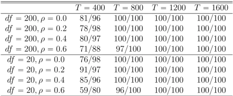
quite good but affected by heavier tails in the innovations in particular in the lag selection case. For the same setup of Π and B as in Table 1, we report model selection results for an almost normal type of innovation withdf “200 and substantial tail thicknessdf “20 across different levels of strength in the cross-sectional correlation Σw in Table 2. The
results show that even for substantial correlation with ρ “ 0.6, performance is reliable
for T ě 800 even in the case of for df “ 20 innovations with excess-kurtosis of 0.375. Generally, a larger degree of freedom leads to better rank selection results given the same T and ρ. Besides, simulations show that the size of ρ has a significant effect on model selection, which highlights the importance of Assumption 2.1 on the structure of Σw, i.e,
the column-wise sums of absolute values must converge fast enough.
T “400 T “800 T “1200 T “1600 df “200, ρ“0.0 81/96 100/100 100/100 100/100 df “200, ρ“0.2 78/98 100/100 100/100 100/100 df “200, ρ“0.4 80/97 100/100 100/100 100/100 df “200, ρ“0.6 71/88 97/100 100/100 100/100 df “20, ρ“0.0 76/98 100/100 100/100 100/100 df “20, ρ“0.2 91/97 100/100 100/100 100/100 df “20, ρ“0.4 85/96 100/100 100/100 100/100 df “20, ρ“0.6 59/80 96/100 100/100 100/100
Table 2: Model selection results for model 1 withm“20, rankr“5, lagp“1 andγ“3
df “20 df “200 T “400 T “800 T “400 T “800 γ “2 ρ“0.0 89{91 98{100 89{92 99{100 ρ“0.4 78{82 97{100 75{88 94{100 γ “3 ρ“0.0 76{98 100{100 81{96 100{100 ρ“0.4 85{96 100{100 80{97 100{100 γ “4 ρ“0.0 46{99 100{100 48{97 100{100 ρ“0.4 50{99 100{100 48{97 100{100
Table 3: Model selection results for model 1 with m “ 20, rank r “ 5 and lag p “ 1 for different ρ
cross-section dependence with differentγ-choices.
model selection in finite sample in the same setting of model 1. In small samples,γ “3 is generally the best choice for consistent rank and lag selection. But withγ “2 only slighly weaker results are obtained, while larger choices increase the weight in the penalty too much and yield substantially less appealing results across all considered tail specifications, cross-correlations and samples sizes. Generally, in the case of model 1 with 20 dimensions andr “5,p“1, the results demonstrate that with a sample size ofT “800 we get 100% perfect rank selection across all cross-correlation and tail scenarios given non-Gaussian innovations. Compare this to usual simulation evidence in high-dimensional set-ups as e.g in Zhang, Robinson and Yao (2018) which exclusively use Gaussian innovations and require sample sizes of T “2000 for comparable performance.
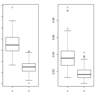
Besides, we present the estimation error of the loading matrix ˆR1 and the cointegrating
space ˜S1 in Figure 1 fordf “20 and in Figure 2 fordf “200 in the caseρ “0.0. Because
α and β are only unique up to rotation, the estimation error here is measured by using orthogonal projection matrices to uniquely identify subspace distances. In particular, we employ the R package LDRTools based on average orthogonal projection matrices proposed by Liski et al. (2016). The left bar in each plot corresponds toT “800 and the right one to T “ 1200. The estimation error for the cointegrating space is significantly smaller than that for the loading matrix due to the faster rate of convergence. Moving from sample size 800 to 1200 significantly improves results in both cases.
Model 2 uses the same Π as model 1 but considers only rank selection in VECM without transient dynamics, i.e. setting B “0. Thus the problem is simpler and technically, the
● ● ● ● 1 2 0.2 0.3 0.4 0.5 0.6 0.7 0.8 0.9
Est.Error of Loading Matrix
● ● ● ● ● ● ● ● 1 2 0.02 0.04 0.06 0.08
Est.Error of Cointegrating Matrix
Figure 1: Estimation Error of model 1 (m“20,r“5,p“1) witht-distributed innovations anddf “20
forρ“0 settingγ“3. Results are shown forT “800 marked as case 1 on thex-axis and for case 2 of
T “1200 ● ● ● ● ● 1 2 0.2 0.3 0.4 0.5 0.6 0.7 0.8
Est.Error of Loading Matrix
● ● ●●●● 1 2 0.0 0.1 0.2 0.3 0.4 0.5
Est.Error of Cointegrating Matrix
Figure 2: Estimation Error of model 1 (m“20,r“5,p“1) witht-distributed innovations anddf“200
forρ“0 settingγ“3. Results are shown forT “800 marked as case 1 on thex-axis and for case 2 of
T “1200
T “400 T “800 T “1200 T “1600 df “200, ρ“0.0 100 100 100 100 df “200, ρ“0.2 98 100 100 100 df “200, ρ“0.4 96 100 100 100 df “200, ρ“0.6 75 100 100 100 df “20, ρ“0.0 98 100 100 100 df “20, ρ“0.2 97 100 100 100 df “20, ρ“0.4 94 100 100 100 df “20, ρ“0.6 74 100 100 100
Table 4: Model selection result for model 2 with m“20, rankr“5, lagp“0 andγ“3
T “400 T “800 T “1200 T “1600
df “200, ρ“0.0 100 100 100 100
df “200, ρ“0.4 86 99 100 100
df “20, ρ“0.0 99 100 100 100
df “20, ρ“0.4 94 100 100 100
Table 5: Rank selection result for model 2 with m “20, rank r“5, lagp“0 and γ “3 and weakly
dependent innovations.
be found in Table 4. In small samples with T “ 400 and for large ρ, this provides
improvements in comparison to 2. Thus without lags, we get satisfactory performance even in these challenging cases of strong cross-sectional dependence.
To test the performance of our method in case of weakly dependent innovations, we generate the weakly dependent innovations according to a MA(2) process. The innova-tions in the underlying MA process arei.i.d. generated fromt-distribution with degree of freedom 20 and 200 respectively. The weakly dependent innovations are generated by
ut“wt`A1wt´1`A2wt´2
where wt follows t-distribution with covariance Σw “ pρ|i´j|qij as defined before. Besides,
A1 “ pa1,ijq “ p0.8iIi“jq and A2 “ pa2,ijq “ pp´0.4qiIi“jq satisfy Assumption 4.1. As in
Table 1, we set γ “3 and choose λ by BIC. See Table 5 for results. When T ě800, the rank selection results are satisfactory, which is consistent with the theoretical results.
In Table 6, we present the rank selection results for the 50-dimensional case of model 3. Compare this to the usual simulation scenarios the high-dimensional non-stationary time series literature which usually do not go beyond dimension 20 (see e.g. Zhang, Robinson and Yao (2018)). We focus on results for innovations following a t-distribution with df “20 anddf “200 respectively, with ρ“0.0, i.e. Σw “Im only. For both cases,
when T ě 2000, the true rank can be estimated almost 100% correct. The increased sample size reflects the difficulty of the problem in dimensionality.
For the high-dimensional set-ups treated before, there exists no other valid feasible method for model determination against which we could evaluate our technique. There-fore, although our techniques are tailored to the high-dimensional case, we briefly il-lustrate that they can also be employed in standard low dimensions where benchmarks
T “800 T “1200 T “1600 T “2000 T “2400
m“50, df “20 51 64 89 93 99
m “50, df “200 55 78 95 97 100
Table 6: Rank selection result form“50 witht-distributed innovations. ρ“0 andγ“3.
exist. In particular, we compare our methods with the Lasso-type techniques in Liao and Phillips (2015) using the “hardest” of their 2-dimensional models treated with r“1 and p“3. In particular, we set Π “
ˆ
´1 ´0.5
1 0.5 ˙
and B1 “B3 “diagp0.4 0.4q, B2 “0 and
Σw “diagp1.25 0.75q. With 5000 simulation replications we get the following model
selec-tion results: forT “100 we get 100%/86.14% while forT “400 we obtain 100%/99.96% which compare to 99.54%/99.80% and 100%/99.98% by Table 2 in Liao and Phillips (2015). In their other settings, we also found similar comparable performance of the two techniques. Results are omitted here for the sake of brevity but are available on request.
6. Empirical Example4
In this section, we employ our method to study the interconnectedness of the Euro-pean sovereign and key players of the banking system during and after the financial crisis. We use CDS log prices of ten European countries and five selected financial institutions provided by Bloomberg terminal: Germany, France, Belgium, Austria, Denmark, Ire-land, Italy, NetherIre-land, Spain, Portugal, BNP Paribas, SocGen Bank, LCL Bank, Danske Bank, Santander Bank 5. The sovereign countries we choose have different debt levels.
The considered time span is from J an.1,2013 to Dec.31,2016 with 1041 observations. BNP Paribas, SocGen Banks are chosen because they rank among the top three Europe based investment banks in Euro-Zone revenues. The other three banks are selected across EU countries covering the whole span from north to south and representing the variety of different financial market and general economic conditions. Initial Augumented Dicky Fuller tests show that the 15 variables are non-stationary but the first-order differences are stationary.
Figure 1 suggests that there exits a strong co-movement among these components. Using our Lasso procedure, we find that there exist two cointegration relations. Figure 2 gives an impression on the stable time evolution of these cointegrated series. Moreover, the time when the cointegrated series exhibit extreme values coincides with some impor-tant economic events. For example, in the middle of the year 2013, European countries were bargaining over the solution for the sovereign debt crisis while at the beginning of 2016 there occurred an economic slowdown in the key global economies.
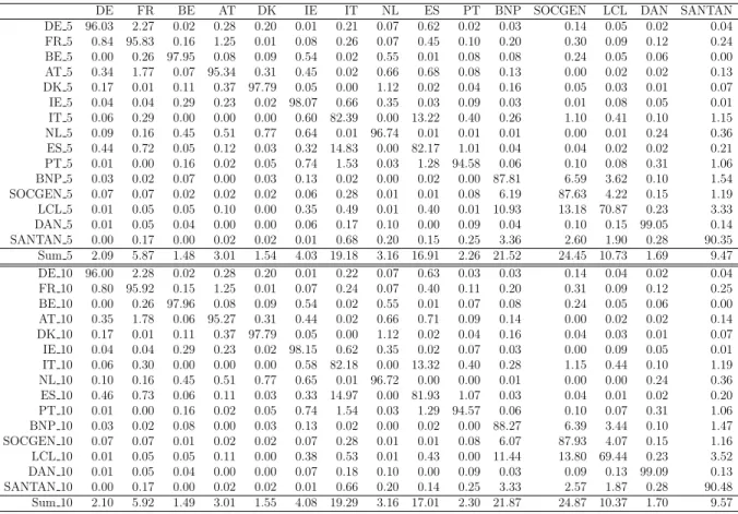
To present the inter-connections among these 15-dimensional VECM components, we calculate the forecast error variance decomposition (FEVD henceafter) due to the
coin-4All the figures for this section can be found in online supplementary
tegrated part, i.e., the forecast error variance decomposition6 derived from (3). From
Table 7 reporting the FEVC results for a 5-and 10-step forecast horizon, we can conclude that leading economies in European Union, such as Germany, are neither risk-exporter nor risk-importer in the whole system.) Italy is the largest risk-exporter among the considered sovereign countries and Spain ranks second. Moreover, Italy and Spain have significant mutual influence on each other. The banks have stronger interconnectedness among themselves than with the sovereign countries. Moreover, Figure 3 shows the con-tribution of Italy to the FEVD of other variables in the full horizon from step 0 to 30, which is consistent with the results in Table 7.
7. Conclusion
This paper discusses how to determine high dimensional VECM under quite general assumptions. It proposes a general groupwise adaptive Lasso procedure which is easily implementable and thus ready to use for practitioners. We show that it works under quite general assumptions such as mild moment conditions on the innovations while rank and dimension can increase with sample sizeT. In particular, consistency results in rank and lag selection are obtained for dimension m satisfying m “OpT1{4´εq for some small
and positive ε. Besides, we also derive the statistical properties of the estimator in case of weakly dependent innovations. According to our best knowledge, this paper is the first to provide a theoretically justified solution to model determination of VECM in a high-dimensional set-up. Questions like efficient estimation of the cointegrating space and faster diverging rates in the dimension require different approaches and thorough investigation. They are therefore left for future research.
References
Ahn, S.K., Reinsel, G.C., 1990. Estimation for partially nonstationary multivariate au-toregressive models. Journal of the American Statistical Association 85, 813–823. Basu, S., Michailidis, G., 2015. Regularized estimation in sparse high-dimensional time
series models. Ann. Statist. 43, 1535–1567.
Bickel, P.J., Levina, E., 2008. Covariance regularization by thresholding. The Annals of Statistics , 2577–2604.
Bickel, P.J., Ritov, Y., Tsybakov, A.B., 2009. Simultaneous analysis of lasso and dantzig selector. Ann. Statist. 37, 1705–1732.
Boswijk, H.P., Jansson, M., Nielsen, M.O., 2012. Improved Likelihood Ratio Tests for Cointegration Rank in the VAR Model. Tinbergen Institute Discussion Paper 12-097/III. Amsterdam and Rotterdam.
Cavaliere, G., Rahbek, A., Taylor, A.M.R., 2012. Bootstrap determination of the co-integration rank in vector autoregressive models. Econometrica 80, 1721–1740.
Chao, J.C., Phillips, P.C., 1999. Model selection in partially nonstationary vector au-toregressive processes with reduced rank structure. Journal of Econometrics 91, 227 – 271.
Chernozhukov, V., Chetverikov, D., Kato, K., 2013. Comparison and anti-concentration bounds for maxima of gaussian random vectors. doi:arXiv:1301.4807.
DasGupta, A., 2008. Asymptotic Theory of Statistics and Probability. Springer Texts in Statistics, Springer New York.
Engle, R., Granger, C., 1987. Co-integration and error correction: represen- tation, estimation and testing. Econometrica 55, 257–276.
Fan, J., Lv, J., 2008. Sure independence screening for ultrahigh dimensional feature space. Journal of the Royal Statistical Society: Series B (Statistical Methodology) 70, 849–911.
Hubrich, K., L¨utkepohl, H., Saikkonen, P., 2001. A review of systems cointegration tests. Econometric Reviews 20, 247–318.
Johansen, S., 1988. Statistical analysis of cointegration vectors. Journal of Economic Dynamics and Control 12, 231 – 254.
Johansen, S., 1991. Estimation and hypothesis testing of cointegration vectors in gaussian vector autoregressive models. Econometrica 59, pp. 1551–1580.
Knight, K., Fu, W., 2000. Asymptotics for lasso-type estimators. The Annals of Statistics 28, pp. 1356–1378.
Kock, A.B., Callot, L., 2015. Oracle inequalities for high dimensional vector autoregres-sions. Journal of Econometrics 186, 325–344.
Kosorok, M.R., Ma, S., 2007. Marginal asymptotics for the large p, small n paradigm: With applications to microarray data. Ann. Statist. 35, 1456–1486.
Li, H., Li, Q., Shi, Y., 2017. Determining the number of factors when the number of factors can increase with sample size. Journal of Econometrics 197, 76–86.
Liao, Z., Phillips, P.C., 2015. Automated estimation of vector error correction models. Econometric Theory 31, 581–646.
Liski, E., Nordhausen, K., Oja, H., Ruiz-Gazen, A., 2016. Combining linear dimension reduction subspaces. proceedings of ICORS 2015 .
L¨utkepohl, H., 2007. New Introduction to Multiple Time Series Analysis. Springer Pub-lishing Company, Incorporated.
Onatski, A., Wang, C., 2018. Alternative asymptotics for cointegration tests in large vars. Econometrica 86, 1465–1478.
Phillips, P.C., 2014. Optimal estimation of cointegrated systems with irrelevant instru-ments. Journal of Econometrics 178, 210 – 224. Recent Advances in Time Series Econometrics.
Revuz, D., Yor, M., 1991. Continuous martingales and Brownian motion. volume 293 of Grundlehren der Mathematischen Wissenschaften [Fundamental Principles of Mathe-matical Sciences]. Springer-Verlag, Berlin.
Signoretto, M., Suykens, J., 2012. Convex estimation of cointegrated VAR models by a nuclear norm penalty. IFAC Proceedings 45, 95 – 100.
Stewart, G.W., 1984. Rank degeneracy. SIAM Journal on Scientific and Statistical Com-puting 5, 403–413.
Stewart, G.W., Sun, J., 1990. Matrix Perturbation Theory. Academic Press.
Tibshirani, R., 1996. Regression shrinkage and selection via the lasso. Journal of the Royal Statistical Society. Series B 58, pp. 267–288.
Vershynin, R., 2012. Introduction to the non-asymptotic analysis of random matrices. Cambridge University Press. p. 210268.
Wei, F., Huang, J., 2010. Consistent group selection in high-dimensional linear regression. Bernoulli 16, 1369–1384.
Wilms, I., Croux, C., 2016. Forecasting Using Sparse cointegration. International Journal of Forecasting 32, 12561267.
Xiao, Z., Phillips, P.C., 1999. Efficient detrending in cointegrating regression. Econometric Theory 15, 519–548.
Yuan, M., Lin, Y., 2006. Model selection and estimation in regression with grouped variables. Journal of the Royal Statistical Society: Series B 68, 49–67.
Zhang, R., Robinson, P., Yao, Q., 2018. Identifying cointegration by eigenanalysis. Journal of the American Statistical Association 0, 1–12.
Zhao, P., Yu, B., 2006. On model selection consistency of lasso. Journal of Machine Learning Research 7, 2541–2563.
Zou, H., 2006. The adaptive lasso and its oracle properties. Journal of the American Statistical Association 101, pp. 1418–1429.
Zou, H., Hastie, T., 2005. Regularization and variable selection via the elastic net. Journal of the Royal Statistical Society: Series B (Statistical Methodology) 67, 301–320.