The Performance and Limitations of ϵ- Stealthy Attacks on Higher Order Systems

The Performance and Limitations of

-Stealthy Attacks

on Higher Order Systems

Enoch Kung, Subhrakanti Dey, and Ling Shi

are of vital importance as the failure of such system can have catastrophic effects. Detection methods can be em-ployed to sense the existence of an attack. In a previous study of an attack on the controller while avoiding detection in scalar systems under a certain control assumption, the notion of-stealthiness was introduced and the strength of

-stealthy attacks was fully characterized. We generalize to the vector system and prove the cases in which we show that the limitations of -stealthy attack do not extend, in the sense that -stealthy can inflict damage of arbitrary magnitude to a vector system.

Index Terms—Cyber-physical systems, detection, secu-rity.

I. INTRODUCTION

In a wireless cyber-physical system (CPS), remote estimation plays a vital role in approximating the system state. However, this set up is open to many forms of potential cyber or physical attacks. Therefore, it is essential for one to devise an accurate estimation method as well as study the effects of attack on a given system. This note will be about the latter.

The security of a CPS is and will continue to be a central topic of study. Communication, transportation, and utility networks are just a few examples of vital systems to modern society. Wireless communi-cation increases the scale of the CPS cheaply but exposes the system to unconventional problems. The compromising of security such as the case of the Maroochy Water Breach [5] and the SQL Slammer worm attack on the nuclear plant [6] emphasizes the importance to study CPS security.

In a typical control system, a plant, sensor and estimator re-quire constant communication, while exposed to natural or malignant sources of corruption. Attackers choose the form and the placement of the attack based on their own ability and purpose. For example, a denial-of-service attack [7] simply prevents a packet of information from successfully transmitting, decreasing the estimation quality. An attacker may also replace the transmitted packet with malicious infor-mation [4] further leading the system astray. Therefore, methods of defense must be developed to ensure an acceptable degree of system performance.

One line of defense is to detect the presence of an attack. A detection policy is a protocol in which an estimator decides whether the received Manuscript received January 20, 2016; revised April 27, 2016; accepted April 29, 2016. Date of publication May 9, 2016; date of current version January 26, 2017. This work was supported by RGC General Research Fund 16210015. Recommended by Associate Editor M. L. Corradini.

E. Kung and L. Shi are with the Department of Electronic and Computer Engineering, Hong Kong University of Science and Tech-nology, Clear Water Bay, Kowloon, Hong Kong (e-mail: [email protected]; [email protected]).

S. Dey is with the Department of Engineering Sciences, Uppsala University, 751 21 Uppsala, Sweden (e-mail: Subhrakanti.Dey@signal. uu.se).

Color versions of one or more of the figures in this paper are available online at http://ieeexplore.ieee.org.

Digital Object Identifier 10.1109/TAC.2016.2565379

data is corrupted. For instance, with a false data injection attack with multiple sensors, a sensor network can verify the validity of one sensor’s data by its neighboring sensors [2], [3]. Detection imposes on the attacker a tradeoff; it must maximize its attack but remain invisible. In [1], a scalar control system under a control assumption is consid-ered in which an attacker may alter the control input constructed by the estimator. The authors then introduced the notion of-stealthiness; the attacker remains undetected if the corrupted output does not differ from a reference exceeding under KL divergence. Under such a detection, the paper provides an-stealthy attack which maximizes the average error covariance. Because it is much more practical to study vector systems, a worthwhile task is to explore these results in a system of higher dimensions and study if, and the extent to which, these results carry over.

In this work, we consider the control system in [1] in a multivariate setting, where an attacker may launch an-stealthy attack. Two scenar-ios are analyzed. One is when the state and output variables are equal in length and the other is when the state vector is longer than the output vector. In these two cases, the effect of-stealthy attacks are different. The tradeoff between the magnitude of damage inflicted to the system and the stealthiness of such attack is only evident in the former case, but not the latter. The main contributions are as follows:

1) In the former scenario, we will provide an upper bound to the average covariance achievable by an -stealthy attack. An -stealthy attack is constructed that achieves our upper bound. Along the way, the relationship between this upper bound and the system parameters, which was not evident in the scalar case, is made explicit.

2) In the latter case, we construct a stealthy attack which is ca-pable of setting the average covariance to be arbitrarily large, thereby proving that there exists no upper bound to the average covariance similar to the one in the previous case.

The note is organized as follows. In Section II, the problem will be formulated after a brief summary of the concepts in [1]. Section III presents the main results, along with their proofs. A numerical simu-lation of the results is given in Section IV. The conclusion is given in the end.

Notations:Throughout this note,Rm×n_{represents the set ofm×}

nreal matrices. LetXbe the transpose ofXandN(μ,Σ)a Gaussian distribution with meanμand covarianceΣ. Denote the set ofn×n symmetric matrices bySn_{, the set of positive semi-definite matrices} bySn

+, and the set of positive definite matrices byS

n

++. SupposeX∈

Sn

++, thenX

1/2_{is the positive definite square root ofX. Define also}

the function δ(x)to be the greater solution to the equationδ(x) = 2x+ 1 + logδ(x).

II. PRELIMINARIES

A. Kalman Filter Consider the system

xk+1=Axk+Buk+wk

yk=Cxk+vk

0018-9286 © 2016 IEEE. Personal use is permitted, but republication/redistribution requires IEEE permission. See http://www.ieee.org/publications_standards/publications/rights/index.html for more information.

whereA, B∈Rn×n_,x

k, uk, wk∈Rn,C∈Rm×n, andyk, vk∈Rm. The noise variables wk, vk are independent and follow the distribu-tions N(0, Q) and N(0, R), respectively. The initial state x0 is a

zero-mean Gaussian variable that is independent of wk and vk. It is assumed that(A, C) is observable and(A, Q1/2_{)is controllable.}

These parameters are known to both the estimator and the attacker. The matrix B is assumed, similar to [1], to be invertible. Further-more, for simplicity,Bcan be considered to beI. This does not hinder the results, and will only slightly affect the form of the constructed attack in Theorem III.3.ii and in Theorem III.4.

The problem of estimating the statexkgiven the output vectorykis solved by the Kalman filter. The Kalman filter is a set of equations from which an estimatexˆkcan be obtained such that the error covariance betweenxˆkandxkis minimized; this estimate is named the minimum mean-squared error (MMSE) estimate. Writing

ˆ

xk=E[xk|y1, . . . , yk]

Pk=E[(xk−xˆk)(xk−ˆxk)|y1, . . . , yk] the Kalman filter are as follows:

ˆ xk+1=Axˆk+Kk(yk−CAxˆk) +uk Pk+1|k=APkA+Q Kk+1=Pk+1|kC[CPk+1|kC+R]− 1 Pk+1= (I−KkC)Pk+1|k whereKkis the Kalman gain.

By the observability and controllability conditions mentioned, the terms {Kk} and {Pk} converges exponentially to a steady-state Kalman gainKand error covarianceP, respectively. Hence, we may assume steady-state has been achieved. The steady-state covarianceP is positive semi-definite solution tog◦h(X) =X, where

g(X) =X−XC[CXC+R]−1CX h(X) =AXA+Q

andK=h(P)C[Ch(P)C+R]−1_.

B. Attack Model

We employ a model in which the attacker corrupts the control vector by altering it arbitrarily. Denote byIkto be the attacker’s information set at timek. The setIkmust satisfy:

1) uk∈Ikfor allk; 2) Ik⊂Ik+1;

3) Ikis independent of all noise{vi}1∞and{wi}∞1 .

The system dynamics can be written as

˜

xk+1=Ax˜k+ ˜uk+wk

˜

yk=Cx˜k+vk (1)

assumingCis full rank, and the estimation equation is

ˆ

xk+1=Axˆk+Kzk+uk. (2) The termzk=yk−Cxˆk∼ N(0, CP C+R)is the innovation. In absence of an attack, this estimation is the MMSE estimate. However, since the plant is now influenced by the corrupted control, the estima-tion is no longer optimal.

The sub-optimal estimator leads to a higher estimation error, and it is the objective of the attack to maximize this error, which is quantified by the performance metric

J= lim sup k→∞ 1 k k i=1 trP˜i

whereP˜i=E[(˜xk−xˆk)(˜xk−xˆk)]. This metric is the average error covariance over an infinite time horizon.

C. Stealth Model

We will give a brief outline of-stealthiness as described in [1]. The estimator, not knowing the presence nor the style of attack performed upon it, may establish a detection policy based on the output vectors

{yi}k₁to raise alarms when there is evidence of an attacker’s presence. At timek, the estimator obtains the outputs{y1, . . . , yk}, which it uses to perform a hypothesis test on the two hypotheses

H0 : Attack does not exist

H1 : Attack exists.

Writing

Pk(H1|H0) =pF Ak (False Alarm)

Pk(H1|H1) =pDk (Detection)

the definition of-stealthiness is introduced in the following.

Definition II.1 (-Stealthiness) [1]: For0< δ <1, an attack is -stealthy if for any detector that satisfies0<1−pD

k ≤δ lim sup k→∞ − 1 klog pF A k ≤.

It is proven in the paper that this is equivalent to the following condition.

Definition II.2:A sequence of attacks{uk}is-stealthy for the resulting innovations{z˜k 1} lim sup k→∞ 1 kD ˜ zk1z k 1 ≤ whereD(˜zk

1z1k)is the KL divergence betweenz˜1kandz1k, i.e.,

Dz˜k 1z k 1 = ∞ −∞ logfz˜ zk 1 fz zk 1 f˜z zk 1 dzk 1.

The KL divergence describes the “difference” between two distri-butions. Here, theparameter acts as a degree of tolerance for the difference between thez˜k

1, which is the innovation corrupted by attack,

andzk

1, which is the innovation if not under attack. Hence the attacker

avoids being detected if its attack can retain this difference under.

D. Problem Setup

Given the system (1) and estimator (2), the goal is to find the max-imum ofJthat can be afflicted on the system by an-stealthy attack. This question is answered for the scalar casem=n= 1in [1], where an upper bound toJis calculated and a stealthy attack is constructed that reaches this bound.

In this note, we continue to look at the optimization

maxJ= max u∞₁ klim→∞ 1 k k i=1 trP˜iwhere{u∞1 } is−stealthy

It will be shown, however, that higher order systems are not as tame and similar results do not always hold. In particular, ifm < n, the -stealthy criterion does not limit the power of the attack, in the sense that there exists an-stealthy attack that can makeJarbitrarily large. The answer provided in [1] can be extended nicely only for the case wherem=n.

III. RESULTS

As oppose to the scalar case, the vector system can be divided into two cases:m=nandm < n. The case in whichm > nis in fact a subcase ofm=n. The former case is solved by providing an upper bound ofJ and the optimal-stealthy attack that reaches the bound. For the latter case, we will prove that the attacker can design an -stealthy attack of arbitrary power.

A. m=n

We begin the analysis by defining several terms

˜ Pi=E[(˜xi−xˆi)(˜xi−xˆi)], Θ˜i=CP˜iC+R Σ =CP C+R, Dk= 1 kD ˜ zk 1z k 1 Ui=E[˜ui−ui].

Remark: Θ˜iis not the covariance of the distribution ofz˜ibecause

˜

Θi=E[˜ziz˜i]and it is not assumed that the mean ofz˜iis 0, unlike the Kalman innovationzi.

An attack is stealthy if the innovation it produces,{z˜k

1}, satisfies lim k→∞ 1 kD ˜ zk1z k 1 = lim k→∞Dk≤.

The termDkcan be expanded, after considerable calculation, to be

Dk=− 1 kh ˜ z1k +1 2log ((2π) n_| Σ|) + 1 2k k i=1 trΣ−1Θ˜i. (3) Here,h(˜zk

1)is the differential entropy of˜z1k. We may then obtain the

inequality 1 2k k i=1 trΣ−1Θ˜i=Dk+ 1 kh ˜ z1k −1 2log ((2π) n_| Σ|) ≤Dk+ 1 k k i=1 h(˜zi)− 1 2log ((2π) n_| Σ|) ≤Dk+ 1 2k k i=1 log (2πe)n_|Σ˜ i| − 1 2k k i=1 log ((2π)n_|Σ|) =Dk+ n 2 + 1 2log _k i=1 |Σ−1_Σ˜ i| 1 k ≤Dk+ n 2 + 1 2log _k i=1 |Σ−1_Θ˜ i| 1 k . The final inequality is justified as follows. By the equationE[(x− μ)(x−μ)] =E[xx]−μμ, the covariance of z˜i is Σ˜i= ˜Θi−

CUiUiC. Since CUiUiC is positive semidefinite, the inequality

˜

Θi≥Σ˜i holds. Furthermore, both Θ˜i and Σ˜i are positive definite, hence|Θ˜i| ≥ |Σ˜i|. The inequality follows by the fact that log is an increasing function. The others are results of the subadditivity of differential entropy and the maximum entropy theorem [1].

It is a known fact that the eigenvalues of Σ−1_Θ˜

i are equiv-alent to those of Σ−(1/2)_Θ˜

iΣ−(1/2). Denote the eigenvalues of

Σ−(1/2)_Θ˜

iΣ−(1/2) by λij. Translating the above inequality using

these eigenvalues, we have

1 2k i,j λij≤Dk+ n 2+ 1 2k i,j logλij. (4)

The following two lemmas are useful tools in the proof of the the main result.

Lemma III.1:If{λij}satisfies the equality of (4), then there exists

{ij}such that λij=δ(ij)and 1 k i,j ij=Dk.

Proof: If equality of (4) holds, then it is not possible for alli, j to satisfy 1 2λij> Dk n + 1 2+ 1 2logλij.

Without losing generality, assume that

1 2λ11≤ Dk n + 1 2+ 1 2logλ11.

Since it is also known that

1 2λ11≥ 1 2+ 1 2logλ11

there must exist11∈[0, Dk/n]such that

1 2λ11=11+ 1 2+ 1 2logλ11

that is,λ11=δ(11). This can be subtracted from both sides of (4) to get

1 2k (i,j)=(1,1) λij= (Dk−11)+ n 2− 1 2k + 1 2k (i,j)=(1,1) logλij.

Repeat the same reasoning to obtain subsequent values ofijsuch that

λij=δ(ij). Plugging this back to (4) so that equality is satisfied, then

Dk+ n 2+ 1 2k i,j logλij= 1 2k i,j λij= 1 2k i,j δ(ij) = 1 2k i,j [2ij+ 1 + logδ(ij)] = 1 2k i,j [2ij+ 1 + logλij].

Canceling terms on both sides results in kDk=

i,j

ij.

Lemma III.2: Let X= (xij)∈S++n with its eigenvalues s1≥

· · · ≥sn≥0andY ∈Snwith eigenvaluesy1≥ · · · ≥yn. Then

tr(XY)≤s1y1+· · ·+snyn.

Proof: By the symmetry ofY, there exists orthogonalQsuch that Y =QY Q¯ , where Y¯ = diag (y1, . . . , yn). Then tr(XY) =

tr(QXQY¯). Since QXQ is positive semi-definite, it can be as-sumed without loss of generality thatY is already diagonal.

Suppose xk fork= 1, . . . , nare the diagonal elements ofX in decreasing order. By the rearrangement inequality

tr(XY) =x11y1+· · ·+xnnyn≤x1y1+· · ·+xnyn. Furthermore, asXis symmetric, by the Schur-Horn Theorem [9], the eigenvalues ofXmajorizes its diagonal, that is

r j=1 xj≤ r j=1 sj, r= 1,2, . . . , n.

Then tr(XY)≤x1y1+· · ·+xnyn =yn _i j=1 xj + n−1 i=1 (yi−yi+1) _i j=1 xj ≤yn _i j=1 sj + n−1 i=1 (yi−yi+1) _i j=1 sj =s1y1+· · ·+snyn.

This lemma shows that the maximization oftr(XY)rests solely on

properly selecting eigenvalues.

The following theorem is the main result of this section.

Theorem III.3: Suppose m=nand Cis invertible, its inverse denoted byE. Then i) J= lim k→∞ 1 k k i=1 trP˜i≤trP+ n j=1 sj δ∗j()−1 .

wheresjare the eigenvalues ofΣ1/2EEΣ1/2withs1≥ · · · ≥

snandδ∗j()are defined by

sj s1 = 1− _δ1∗ j 1− 1 δ∗₁ and2= n j=1 δj∗−logδ∗j−1.

ii) There exists an attack u˜∞₁ that the resulting P˜i achieves the upper bound.

Proof of I: The proof of the theorem will be carried out in the following way as we aim to boundtrP˜i. Suppose that it is possible for the bounding oftrP˜ito be transformed to the bounding oftr(XY), whereX∈Sn

++is fixed by the system, andY ∈Snis free to design

under constraint. Then the upper bound is dependent solely on the eigenvalues ofXand an appropriately selected eigenvalue ofY by the second lemma. The first lemma then reveals the set of eigenvalues we can choose from. From this set of eigenvalues, Lagrange multipliers will be carried out to find the optimal eigenvalues that yields the desired bound.

To transform the maximization problem, we notice that trP˜i=trP+tr E( ˜Θi−Σ)E =trP+tr Σ12EEΣ 1 2 Σ−12Θ˜_iΣ− 1 2−I . (5)

The first term is constant, hence we want to bound the second term. The matrixΣ1/2_EEΣ1/2_∈Sn

++andΣ− (1/2)_Θ˜

iΣ−(1/2)−I∈Sn, hence Lemma III.2. can be applied. The former term is fixed by system parameters, whereas the second term includesΘ˜i, which is determined by the attacker.

If we represent their eigenvalues as{sj}and {Λ˜ji}, respectively, listed in decreasing order, the lemma yields

tr Σ12_EEΣ12 Σ−12_Θ˜_iΣ−12 −_I ≤_Λ˜1 is1+· · ·+ ˜Λnisn. (6) The remaining task is to maximize (6) through a correct selection of

{_Λ˜j

i}while satisfying (4), i.e.,

−n 2 − 1 2k i,j log ˜ Λj_i+ 1 +1 2 1 k i,j 1 + ˜Λj_i ≤Dk. (7) The expression on the left side is an increasing function for positive

˜

Λj_i, meaning that if the inequality is strict, one may increase anyΛ˜j_i,

which in turn increases (6). In other words, the optimal choice ofΛ˜j_i∗

must satisfy equality of (7), paving the way for us to use Lemma III.1. The lemma guarantees the existence ofijsuch that

1 + ˜Λj_i =δ(ij)and 1 k i,j ij=Dk.

With these new terms, the maximization of (6) becomes

max i,j sj(δ(ij)−1) subject to 1 k i,j ij=Dk. (8)

Recall thatδ(x)solvesδ(x) = 2x+ 1 + logδ(x), so the constraint can be rephrased as 1 2k i,j δ(ij)−1−logδ(ij) =Dk

and instead of usingijas our variables, we can takeδ(ij)to be the

variables. Naturally, Lagrange multipliers can be employed to solve for optimal valuesδ∗(ij). Solving

∇ i,j sj(δ(ij)−1) =η∇ 1 2 i,j δ(ij)−1−logδ(ij)

gives us the equation

(s1, . . . , sn) =η 1 2 1− 1 δ(11) , . . . ,1 2 1− 1 δ(kn) . Thus the optimal valuesδ∗(ij)must satisfy the equations

sj s1 = 1− 1 δ∗(ij) 1− 1 δ∗(11) for alli, j 2Dk= n j=1 δ∗(ij)−logδ∗(ij)−1

Note that these optimal valuesδ∗(ij)are dependent onDkandjbut not oni, hence they can be denoted byδ∗j(Dk).

This results in the upper bound of (5) trP˜i=trP+tr QiΣ 1 2_EEΣ12_QiΛ˜_i ≤trP+ n j=1 sj δj∗(Dk)−1 which immediately leads to

J= lim k→∞ 1 k k i=1 trP˜i ≤ lim k→∞ 1 k k i=1 trP+ n j=1 sj δ∗j(Dk)−1 = lim k→∞trP+ n j=1 sj δ∗j(Dk)−1 =trP+ n j=1 sj δ∗j( lim k→∞Dk)−1 ≤trP+ n j=1 sj δ∗_j()−1.

Clearly, this proof extends the results from [1] because in the scalar case, the eigenvalue of Σ1/2_EEΣ1/2 _{equals σ}2

z/c

2 _{and δ}∗

simplyδ(). Then, given thatσ2 z=c2P+r trP+s1 δ∗_j()−1=P+σ 2 z c2 (δ()−1) =δ()P+(δ()−1)r c2 .

This is the result of [1].

Proof of II: In this proof, we first propose an attack. Then we verify that it indeed reaches the upper bound stated in Theorem III.3. and is-stealthy.

DefineQto be the matrix that diagonalizesΣ1/2_EEΣ1/2_{, i.e.,}

QΣ12EEΣ21Q=S= diag (s₁, . . . , s_n).

Also, let {ζk} be a sequence of Gaussian random variables of distributionN(0, EΣ1/2_QΛQΣ1/2_{E), where Λ = diag (δ}∗

1()−

1, . . . , δ_n∗()−1). Define an attack by

˜

uk=uk−(A−KC)ζk−1+ζk (9) withζ1= 0. To facilitate the verification of this construction’s validity,

define an intermediate processxs

kdefined by xs k+1=Ax s k+K(yk−Cxsk) + ˜uk with xs

1= 0. This yields the MMSE estimate of the state xk, in particular,E[(xs

k−xk)(xsk−xk)] =P. Ifek= ˆxk−xsk, we have

˜

zk=yk−Cxˆk= (yk−Cxsk)−Cek

ek+1= (A−KC)ek+ (A−KC)ζk−1−ζk. (10) Givene1= 0, the solution to the second recursion isek=−ζk−1.

It can now be verified that trP˜i=E (ˆxi−xsi)(ˆxi−xsi) +E (xsi−xi)(xsi−xi) + 2E (ˆxi−xsi)(xsi−xi) =trP+trEekek =trP+trSΛ =trP+ n j=1 sj δ∗_j()−1 and consequently J= lim k→∞tr ˜ Pi=trP+ n j=1 sj δ_j∗()−1

which is our stated upper bound.

It remains to show that this attack is-stealthy. By (10), it is imme-diate that z˜i∼ N(0,Σ1/2[I+QΛQ]Σ1/2). Since Σ˜i= Σ1/2[I+

QΛQ]Σ1/2_{, a quick calculation shows}

tr(Σ−1_Σ˜ i) =tr(I+ Λ) = n j=1 δ∗j() |Σ−1Σ˜i|=|I+ Λ|= n j=1 δj∗().

Plugging this into(3), noting that the differential entropy(1/k)h(˜zk

1) = (1/2) log(2πe)n₍k i=1|Σ˜i|) 1/k ifz˜k 1 is Gaussian, we have −n 2 − 1 2log _k i=1 |Σ−1_Σ˜ i| 1 k + 1 2k k i=1 trΣ−1_Σ˜ i =−n 2 − 1 2 n j=1 logδ∗_j() +1 2 n j=1 δ_j∗() =.

IfBis a general invertible matrix, then (9) would be rewritten as B˜uk=Buk−(A−KC)ζk−1+ζk.

The attack would take the form

˜

uk=uk−B−1(A−KC)ζk−1+B−1ζk.

Finally to settle the casen < m, supposeC∈Rm×n_{and full rank.} Intuitively, ifCis one-to-one, then all of the information in the state variable should roughly be encoded into the output, hence should not be any different from the case whenCis square. In detail, there exists an invertible matrix row operationC¯∈Rm×m_{such that}

C= ¯C

I 0

which when substituted into the system equations renders yk=Cxk+vk= ¯C xk 0 +vk.

SinceC¯is a square, full rank matrix, the results obtained in this section extends to this scenario.

B. m < n

In this section, it will be shown that the detection employed by the estimator is not effective in a vector system against-stealthy attacks in the sense that there exist an -stealthy attack that can arbitrarily increaseJ.

Theorem III.4:Letm < nand assume thatCis full rank. There exists an attacku˜∞1 such that from its produced error covariance{P˜i}, the performance metricJcan be arbitrarily large.

Proof: Note that by the surjectivity of C, there exists an invertible matrix C¯ such that C= [I 0] ¯C. Suppose we find a Σ˜

satisfying (4), then writing

¯ CP˜iC¯= _¯ P1 i P¯i2 ¯ P3 i P¯ 4 i (11) will result in the equality

CP˜iC= ¯Pi1= ˜Σ−R.

This means that the other submatrices are degrees of freedom which may causeJto diverge. For example, chooseP¯2

i = ¯Pi3= 0andP¯i4=

αIfor someα. Then tr _¯ P1 i 0 0 αI =trC¯P˜iC¯ =trP˜iC¯C¯

which by the inequality trAB≤tr(A)tr(B) for positive definite matricesA, B[8] trP˜i≥ tr _¯ P1 i 0 0 αI trC¯C¯ . (12) WithP¯1

i andC¯C¯being constant for a fixedandC, it is straight-forward to see that the selection ofαcan arbitrarily increase the term

lim

k→∞(1/k) k

i=1trP˜i.

With this strategy in mind, letζk∼ N(0, Z), whereZsatisfies

¯ CZC¯= δ n −1Σ 0 0 βI .

Fig. 1. J1: upper bound;J2:ij=/n;J3:ij= 2j/n(n+ 1);J4:ijis

random.

As with the proof of Theorem III.3., define the attack

˜

uk=uk−(A−KC)ζk−1+ζk or ifB=I

˜

uk=uk−B−1(A−KC)ζk−1+B−1ζk. It can now be verified that

trP˜i=trE ekek +trP ≥ 1 trC¯C¯ tr δ n −1 Σ + (n−m)β +trP. (13) Sinceβcan be arbitrarily large, so canlimk→∞(1/k)ki=1trP˜i.

The final requirement is to prove that this attack is-stealthy. By (10), it follows thatz˜k∼ N(0, δ(/n)Σ), that is,Σ˜i=δ(/n)Σ. So

1 kD ˜ zk 1z k 1 = n 2δ n −n 2− n 2logδ n =n 2 2 n =. Hence our constructed attacku˜kis-stealthy.

IV. NUMERICALRESULTS

The two results will be illustrated by numerical examples. It can be seen that when m=n, no other average covariances obtained from stealthy attacks can exceed the stated bound. As for the second result, the average covariance resulting from the proposed attack in the previous section is shown to increase indefinitely withβ.

ForFig. 1, we used A= 1 1 0 1 , C= 3 4 1 1 Q=R= 0.6 0 0 0.3 , = 0.1.

The dependent variable is the term(1/k)k_i=1trP˜i, which conve-niently can be denoted by J(k). Aside from the upper bound, the other average covariances are obtained by choosing {ij}satisfying

the constraint lim k→∞ 1 k i,j ij=.

J2 is obtained by takingijto be constant;J3 is obtained by letting

i1= 2/(n(n+1))andi2= 2i1, i3= 3i1, . . . , in=ni1;J4is

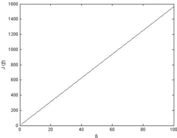
Fig. 2. Average covariance described in partBdependent onβ.

obtained by randomly selectingijsuch that the constraint is satisfied.

Ask→ ∞,J1is the highest.

The reason thatJ4is greater thanJ1for smaller values ofkis that

the optimal values{δ_j∗}for the optimization problem (8) whenDk= is not the optimal values for other choices ofDk. Therefore, it is pos-sible that the optimal values for a certainDk=can achieve a higher average covariance at timekthan{δ∗_j}. However, the assumption that Dktends toaskincreases implies thatJ4(k)must sink below our

upper bound ask→ ∞which is evident in this example. Form < n, the parameters are

A= 1 1 0 1 , C=3 4 Q= 0.6 0 0 0.3 , R= 0.6, = 0.1. Then by the proposed attack in the previous section, taking

Z= ¯C−1 δ n −1Σ 0 0 βI ( ¯C)−1 we acquire lim k→∞ 1 k i ˜ Pi=trZ+trP

which can be denoted by J(β). By simple observation, this value increases linearly byβ; this is shown in theFig. 2.

V. CONCLUSION ANDFUTUREWORK

In the framework of-stealthiness, we aim to study the estimation performance under a stealthy attack. In this work, we specify in higher dimensions the situation where results carry from [1] and when they do not hold. In the vector case, one can see the interplay between system parameters with greater clarity. The results further shows that in the more practical setting, with short output vectors and long state vectors, the-stealthiness detection method is ineffective in preventing an attack.

The next step naturally is to consider the defence against-stealthiness when m < n. The objective of the controller would be to expose the attacker, if present, by maximizing the KL divergence, while the attacker attempts the opposite. In this respect, the problem can be formulated as a two-person infinite horizon dynamic game between the controller and the attacker. This and other defence mechanisms are beyond the scope of this note and will be investigated in future work.

REFERENCES

[1] C. Z. Bai, F. Pasqualetti, and V. Gupta, “Security in stochastic control sys-tems: Fundamental limitations and performance bounds,” inProc. Amer. Control Conf., Chicago, IL, USA, Jul. 1–3, 2015, pp. 195–200. [2] F. Ye, H. Luo, S. Lu, and L. Zhang, “Statistical en-route filtering of

injected false data in sensor networks,” inProc. IEEE Int. Conf. Comput. Commun., 2004, vol. 4, pp. 839–850.

[3] V. Shukla and D. Qiao, “Distinguishing data transience from false injec-tion in sensor networks,” inProc. IEEE 4th Annu. Commun. Soc. Conf. Sens., Mesh Ad Hoc Commun. Netw., 2007, pp. 41–50.

[4] Y. Liu, M. K. Reiter, and P. Ning, “False data injection attacks against state estimation in electric power grids,” inProc. ACM Conf. Comput. Commun. Security, Chicago, IL, USA, Nov. 2009, pp. 21–32.

[5] J. Slay and M. Miller, “Lessons learned from the Maroochy water breach,”

Critical Infrastruct. Protect., vol. 253, pp. 73–82, 2007.

[6] S. Kuvshinkova, “SQL slammer worm lessons learned for consider-ation by the electricity sector,” North Amer. Elect. Reliab. Council, Jun. 2003.

[7] S. Amin, A. Cárdenas, and S. Sastry, “Safe and secure networked control systems under denial-of-service attacks,”Hybrid Syst.: Comput. Control, vol. 5469, pp. 31–45, Apr. 2009.

[8] X. Yang, X. Yang, and K. L. Teo, “A matrix trace inequality,”J. Math. Anal. Appl., vol. 263, pp. 327–333, 2001.

[9] “Uber eine Klasse von Mittelbildungen mit Anwendungen auf die Deter-minantentheorie, Sitzungsber,”Berl. Math. Ges., vol. 22, pp. 9–20, 1923. [10] S. H. Ahmed, G. Kim, and D. Kim, “Cyber physical system: Architecture, applications and research challenges,” inWireless Days, IFIP, Valencia, Spain, Nov. 2013, pp. 1–5.