Workload-sensitive Approaches to
Improving Graph Data Partitioning
Online.
Hugo Firth
Submitted for the degree of Doctor of
Philosophy in the School of Computing
Science, Newcastle University
July 2018
c
Many modern applications, from social networks to network security tools, rely upon the graph data model, using it as part of an offline analytics pipeline or, increasingly, for storing and querying data online, e.g. in a graph database management system (GDBMS). Unfortunately, effective horizontal scaling of this graph data reduces to the NP-Hard problem of “k-way balanced graph partitioning”.
Owing to the problem’s importance, several practical approaches exist, producing qual-ity graph partitionings. However, these existing systems are unsuitable for partitioning online graphs, either introducing unnecessary network latency during query process-ing, being unable to efficiently adapt to changing data and query workloads, or both. In this thesis we propose partitioning techniques which are efficient and sensitive to given query workloads, suitable for application to online graphs and query workloads.
To incrementally adapt partitionings in response to workload change, we propose
TAPER: a graph repartitioner. TAPER uses novel datastructures to compute the probability of expensive inter-partition traversals (ipt) from each vertex, given the current workload of path queries. Subsequently, it iteratively adjusts an initial parti-tioning by swapping selected vertices amongst partitions, heuristically maintaining low
ipt and high partition quality with respect to that workload. Iterations are inexpensive thanks to time and space optimisations in the underlying datastructures.
To incrementally createpartitionings in response to graph growth, we proposeLoom: a streaming graph partitioner. Loom uses another novel datastructure to detect com-mon patterns of edge traversals when executing a given workload of pattern matching queries. Subsequently, it employs a probabilistic graph isomorphism method to in-crementally and efficiently compare sub-graphs in the stream of graph updates, to these common patterns. Matches are assigned within individual partitions if possible, thereby also reducing ipt and increasing partitioning qualityw.r.t the given workload.
ipt by upto 80% over a naive existing partitioning and can maintain this reduction in the event of workload change, through additional iterations. Meanwhile, Loom reduces
I declare that this thesis is my own work unless otherwise stated. No part of this thesis has previously been submitted for a degree or any other qualification at Newcastle University or any other institution.
Hugo Firth
Significant portions of the work presented within this thesis have been documented in the following publications:
JOURNAL
1. H. Firthand P. Missier,TAPER: query-aware, partition-enhancement for large, heterogenous graphs, Distributed and Parallel Databases, 35(2) Special Issue: Distributed Graph Processing and Management, 85-115, June 2017
CONFERENCE
1. H. Firth and P. Missier, Loom: Query-aware Partitioning of Online Graphs, Proceedings of 21st International Conference on Extending Database Technology (EDBT), March 2018
2. H. Firth and P. Missier, ProvGen: Generating Synthetic PROV Graphs with Predictable Structure, Proceedings of 5th International Provenance and Annota-tion Workshop (IPAW), June 2014
WORKSHOP
1. H. Firthand P. Missier,Workload-aware streaming graph partitioning, Proceed-ings of the Joint EDBT/ICDT Workshops (GraphQ), March 2016
I’d like to start by thanking my PhD supervisor, Dr. Paolo Missier, for all his patience, advice and support throughout my studies. I apologise for my tendency to over-engineer: both sentences and programs.
More generally, I’d like to thank some of the people I have worked alongside: Jack Aiston, for his help understanding the arcane mysteries of combinatorics; Naomi Han-naford, both for being really supportive and for suffering through my loudness; finally, Thomas Cooper and Lauren Roberts, who kept things interesting with the occasional much needed distraction.
Thank you to my family, whose support and belief, though occasionally daunting, means the world to me. Huge thank yous to Rob Thompson and Wojciech Mu-sialkiewicz, who are the best team. Finally, and most importantly, love and thanks to my partner Lisa, whose contributions towards who I am are elided for space.
1 Introduction 1
1.1 Graph Partitioning . . . 4
1.2 Motivating problem . . . 6
1.2.1 Workload-agnostic partitioners . . . 7
1.3 Research Aim and Contributions . . . 9
2 Preliminaries 12 2.1 Graph datastructures . . . 13
2.1.1 Graph stream orderings . . . 14
2.2 Graph operations . . . 15
2.3 Graph partitions . . . 18
2.4 Partitioning Quality and Objective Functions . . . 19
2.5 Partitioning Hardness . . . 20
3 Related work 22 3.1 Local graph re-partitioners . . . 23
3.2 Global graph partitioners . . . 26
3.2.1 Spectral techniques . . . 27
3.2.2 Diffusions techniques . . . 28
3.2.3 Multilevel application . . . 29
3.3 Distributed graph partitioners . . . 32
3.4 Streaming graph partitioning . . . 34
3.4.1 Re-streaming . . . 36
3.5 Workload sensitive partitioning . . . 38
3.5.1 Offline workloads . . . 39
3.5.2 Online workloads . . . 40
3.5.3 Replication systems . . . 42
3.6 Comparing partitioner systems . . . 44
3.6.1 System properties . . . 45
3.6.2 Suitability of existing systems to online workload-sensitive par-titioning. . . 46
4.1.1 The TAPER re-partitioner . . . 53
4.1.2 Contributions . . . 55
4.1.3 Related Work . . . 55
4.2 Definitions . . . 56
4.2.1 Stability of a graph partitioning . . . 57
4.2.2 Workload-sensitive stability . . . 58
4.2.3 The Visitor Matrix: Non-random walks with memory . . . 59
4.3 Enhancing a Partitioning . . . 61
4.3.1 Increasing stability by Vertex swapping . . . 61
4.3.2 Introversion and Extroversion . . . 62
4.4 Prefix Trie encoding of query expressions . . . 64
4.4.1 Associating probabilities to trie nodes . . . 66
4.4.2 Computing VM cells with the TPSTry . . . 68
4.5 Implementation . . . 70
4.5.1 Architecture . . . 70
4.5.2 Reducing the cost of the Visitor matrix . . . 71
4.5.2.1 Space complexity . . . 71
4.5.2.2 Time complexity . . . 73
4.5.3 TPSTry Implementation . . . 73
4.5.4 Calculating a partial extroversion order . . . 74
4.5.5 Vertex Swapping . . . 75
4.6 Evaluation . . . 77
4.6.1 Experimental setup . . . 78
4.6.1.1 Test datasets . . . 78
4.6.1.2 Test query workloads . . . 79
4.6.2 Results . . . 81
4.6.2.1 Improvement over an initial hash partitioning . . . 81
4.6.2.2 Improving over other initial partitionings . . . 82
4.6.2.3 The effect of differing numbers of partitions . . . 83
4.6.2.4 Optimising for frequent queries . . . 84
4.6.2.5 The effect of changes in query workloads . . . 85
5.1.1 The Loom partitioner . . . 94
5.1.2 Contributions . . . 96
5.2 Identifying Motifs . . . 97
5.2.1 Sub-graph signatures . . . 98
5.2.2 Constructing the TPSTry++ . . . 101
5.2.3 Avoiding signature collisions . . . 102
5.3 Matching Motifs . . . 105
5.3.1 Building a graph index . . . 110
5.4 Allocating Motifs . . . 111 5.5 Evaluation . . . 115 5.5.1 Experimental setup . . . 115 5.5.1.1 Graph datasets . . . 116 5.5.1.2 Query workloads . . . 117 5.5.2 Comparison of systems . . . 118
5.5.3 Effect of stream order and window size . . . 122
5.6 Conclusion . . . 124
6 Discussion 127 6.1 Thesis Summary . . . 128
6.2 Summary of contributions . . . 130
6.2.1 Properties desirable for online graph partitioning techniques . . 130
6.2.2 Capturing online query workload information . . . 131
6.2.3 Workload-sensitive re-partitioning of existing graphs for online workloads . . . 132
6.2.4 Workload-sensitive partitionings of online, growing graphs . . . 132
6.3 Future research directions . . . 134
6.3.1 Integrating TAPER and Loom . . . 134
6.3.2 Distributing Loom across multiple hosts . . . 135
6.3.3 Restreaming with Loom . . . 136
6.3.4 A timeseries approach to triggering TAPER repartitionings . . . 136
6.3.5 Considering other forms of graph data . . . 137
1.1 Example graph representations of various data models. . . 2
1.2 A 4-way graph partitioning distributed across a cluster of machines . . 5
1.3 Sub-optimal partitioning w.r.t a workload Q . . . 7
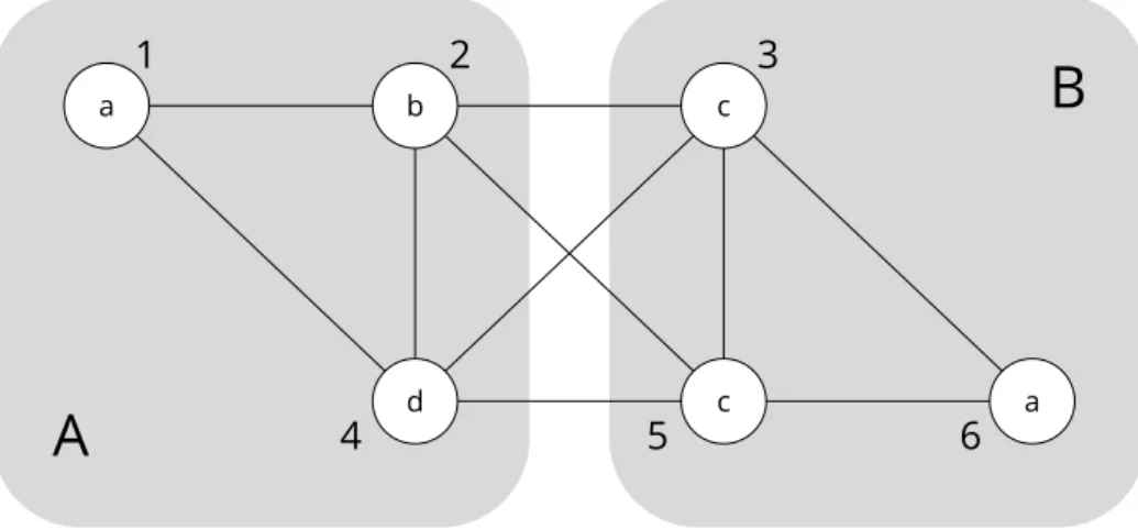
2.1 Example graphG with query workload Q . . . 17
2.2 Vertex vs Edge centric partitionings . . . 18
3.1 The partitioning pattern common to multilevel apparoaches. Inspired by similar figures in [58, 102] . . . 30
3.2 Example of “folding” in distributed mulilevel graph partitioners. . . 33
3.3 Trivial example of an adversarial graph stream ordering. . . 36
4.1 Illustrative example graph . . . 53
4.2 Visitor Matrix structure . . . 60
4.3 Summary trie construction from queries. . . 66
4.4 Visitor Matrix (left), TPSTry probabilities (right) . . . 68
4.5 Architecture . . . 71
4.6 Offer/Receive algorithm in each TAPER instance . . . 76
4.7 ipt perTAPER internal iteration . . . 81
4.8 ipt per approach . . . 83
4.9 ipt vs k partitions (ProvGen) . . . 83
4.10 ipt per query . . . 84
4.11 ipt vs Workload change . . . 84
4.12 ipt over time w. TAPER invocations . . . 86
5.1 Example graphG with query workload Q. . . 94
5.2 TPSTry++ for Qin fig. 2.1 . . . 97
5.3 Combining tries for query graphs q1, q2 . . . 99
5.4 Probability of <5% factor collisions for various p . . . 104
5.5 t-length window over G (left), Motifs from TPSTry++ (center) and motif matchList for window (right) . . . 107
5.8 ipt %, vs. Hash, when executing Q over multiple k-way partitionings
of breadth-firstgraph streams. . . 120 5.9 ipt (y-axis) when executing Q over Loom partitionings with multiple
window sizes t(x-axis) . . . 123
3.1 Properties of Graph partitioners . . . 47
4.1 Properties of the TAPER re-partitioner . . . 88
4.2 Comparison framework properties overview . . . 88
5.1 Graph datasets, incl. size & heterogeneity . . . 118
5.2 Time to partition 10k edges . . . 122
5.3 Comparison framework properties overview . . . 125
5.4 Properties of the Loom partitioner . . . 125
1
Introduction
Contents
1.1 Graph Partitioning . . . 4 1.2 Motivating problem . . . 6 1.2.1 Workload-agnostic partitioners . . . 7Group Person Person Person Post Post Post MemberOf MemberOf MemberOf Follows Submitted Submitted Submitted Journal Paper Paper Author PublishedIn PublishedIn Cited Wrote W rote Protein Protein Function InteractsWith RelatesT o RelatesT o
Social network Protein-Protein interactions Academic publishing
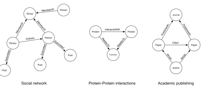
Figure 1.1: Example graph representations of various data models.
Structuring data as a graph, representing records as labelled vertices with inter-connecting edges corresponding to relationships, is increasingly common in many application domains. These include social networks [16, 47, 122], Bioinformatics tools [10, 121] and structured document networks such as academic papers and the world wide, or semantic webs [4, 21, 39].
There are several reasons for this recent prevalence. Notably, graphs are a very natural representation of data, sidestepping issues of complex schema design [5]. Consider the examples presented in Figure 1.1. In a social network a Person record might have a
Submitted relationship with several Post records, along with MemberOf relationships to several Group records. Meanwhile, Bioinformaticians often model the interaction between the proteins in living cells usingprotein-protein interaction(PPI) graphs [121], where vertices may represent individual proteins or the bodily functions to which proteins relate (e.g. cell growth). In a more traditional tabular format, such as found in relational database management systems (RDBMS), the edges in Fig. 1.1 would require structures like pivot tables or data duplication (i.e. denormalisation) to express.
Furthermore, storing data in a graph format also renders many classes of operation efficient and/or simple to express. A classic example of such an operation is the shortest-path query [69]: selecting the smallest possible sequence of edges which connect any two given vertices. Shortest-path queries are often used for physical route planning, or finding chains of social connections, known as “friend-of-friend”. In a
tabular format, each additional “of-friend” step requires an expensive scan of the data or index lookup: a join in RDBMS parlance.
On the other hand, when storing data in a graph format, such queries typically corre-spond to a single index lookup and subsequent traversal of a small number of graph edges. Edge traversal is analogous to pointer dereferencing, significantly faster than an index intensive join [100]. Specialised graph analysis frameworks1, graph database management systems (GDBMS)2 and certain RDF Stores3 exist to exploit these
ad-vantages.
Note that, with the exception of simple aggregation tasks such as finding the average degree4, the majority of graph operations are implemented using a large number of
these efficient edge traversals.
Besides shortest-path, the famous PageRank algorithm [88] can be written as a graph operation [75]. Each document is represented as a vertex with an initial rank. For each vertexv in turn, the algorithm traversesall outgoing edges (links)5 and updates
the rank of all neighbours, based on the rank of v. This process is repeated until the ranks of vertices converge to stability.
Additionally, consider the common follower recommendation feature of social net-works [47]. Given the example in Fig. 1.1, Person a might wish to be recommended other members of their Group who they do not Follow. This is known as a sub-graph pattern matching query, and is implemented in GDBMS as a series of edge-traversals [100] from a given starting vertex (e.g. Person a).
Pagerank is a classic example of an offline analytical operation: a slow running task, often executed as a one-off (offline), e.g. by an analyst, or very infrequently. Sub-graph pattern matching queries may also be executed infrequently, often in large batches, constituting offline analytical operations. However, they are more typically an example of an online data-management operation: a fast and relatively cheap operation often executed automatically and frequently (online). For example, as part
1e.g. Pregel [74], GraphX [124], GraphChi [66] and others 2e.g. Neo4j [86], TitanDB [114], Trinity [108]
3e.g. Apache Jena [14], Virtuoso [30]
4The average number of edges incident to each vertex in a graph.
5In some literature this traversal is referred to as message passing between vertices. For the
of a read request to a GDBMS, to find and return a small number of records; or as part of a write request, to find the area of a graph to update or add to.
Note that online data-management operations are often collectively referred to as On-line Transactional Processing (OLTP). However, we do not use that acronym through-out this thesis, simply referring to operation types in full, or as online/offline. This avoids confusion with types of operation we do not consider, such as online analytical, and with the common misunderstanding that OLTP refers only to operations executed in strongly consistent relational database management systems.
Despite the clear advantages presented above, there are some potential drawbacks to the graph representation of data, namely concerning the efficiency of systems which make use of it at scale. It is the scalability of graph based applications which we aim to improve with this work, particularly in an online context.
1.1
Graph Partitioning
To understand the scalability concerns surrounding graphs, first note that applications from domains where we argue graphs are most useful produce large quantities of data, often continuously. This is especially true of social networks: a widely used Twitter dataset from 2010 [65] contains 1.5 billion Follow relationships, whilst Facebook’s graph data may now contain as many as many as 13 billion vertices [45]. Given such quantities of data, systems must scale up or scale out regardless of representation.
Scaling up describes the process of increasing the effective resources of a single machine, using specialised hardware6 or techniques, in order to process large amounts of data.
Notably, this is the approach taken by the GraphChi analysis framework [66], which applies a “parallel sliding windows” approach to only process a small subset of a graph at any time. The downside to scaling up is that the specialised hardware involved is very expensive and still has some fundamental scalability limits which are difficult to overcome (e.g. network bandwidth).
Scaling out is more common, and usually implies data sharding: splitting data into a number of similar chunks in order to take advantage of the increased resources of
Machine A
Machine B Machine D
Machine C
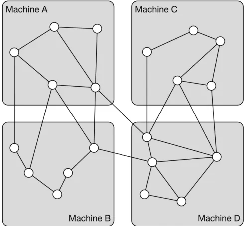
Figure 1.2: A 4-way graph partitioning distributed across a cluster of machines
a homogeneous cluster of machines. Over graph structured data, effective sharding is equivalent to the well-known NP-Complete [3] problem of “k-way balanced graph partitioning”. Each ofk machines in a cluster contains a distinct portion of the graph, known as a partition. Partitions are likely connected by some number of edges, in which case corresponding machines will also contain copies of the connecting elements. Figure 1.2 presents an example of such a partitioning.
To understand why scaling out effectively is challenging for graph based systems, consider Fig. 1.2 and recall that most workloads of graph operations require large numbers of edge traversals, regardless of whether they are offline or online in nature. When a traversal is required over an edge which connects two partitions, intuitively one or more network requests are required; we refer to these as inter-partition traversals (ipt). As network latency is orders of magnitude higher and more variable than main-memory, or even disk access [22], the more ipt an operation causes, the slower its running time.
In order to scale out graph based systems effectively, sophisticated graph partitioners have been proposed [17, 52, 58, 76, 110, 117, 125], the details of which we discuss in Chapter 3. The fundamental goal of these systems is to arrange the vertices and edges of a graph across distributed partitions in such a way that operations may be executed efficiently, with minimal network latency.
1.2
Motivating problem
Despite the challenging nature of the problem, aforementioned existing partitioners are often able to produce good results: graph partitionings which support the efficient execution of operations whilst distributed. This is especially common when given graphs subject to workloads of offline analytical operations. However, these systems are rarely an effective or appropriate choice when given large graphs used in an online context. This lack of graph partitioning systems which are well optimised for online data-management serves as the ongoing motivation for this work.
Broadly speaking, the difference in effectiveness is due to the fact that existing par-titioners make trade offs which are acceptable to an offline system, but incompatible with the requirements of an online one. For instance, most graph partitioners are slow over large graphs, taking on the order of tens of minutes, or even hours [117]. Addi-tionally, most partitioners are not incremental in nature, i.e. if a sub-graph is added to an existing partitioning, the partitioner must be re-executed over the entire graph, not just the new portion.
For offline analytics applications, where the data is often static or updated in infrequent batches, graphs can be partitionedonce prior to an operation. The execution time of an analytics operation may exceed that of even a complex partitioner by several orders of magnitude [125]. Therefore, if a quality graph partitioning reduces the operation’s execution by (e.g.) 30% then the upfront cost of the partitioner is worthwhile.
Meanwhile, in online data-management applications graphs grow continuously, which requires repeated re-execution of expensive non-incremental partitioners. As consis-tent availability and performance is paramount online, such existing partitioners are rendered impractical [55].
Machine A
Machine B Machine D
Machine C
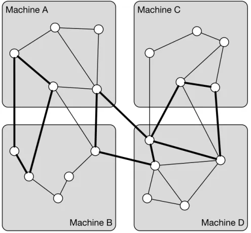
Figure 1.3: Sub-optimal partitioning w.r.t a workloadQ
More importantly, even existing incremental [52,87,110,117] partitioners may produce sup-optimal partitionings in an online context because they optimise for an inappro-priate goal.
1.2.1
Workload-agnostic partitioners
Recall that when partitioning graphs to scale out effectively, our primary aim is to minimise the network latency when executing operations (Sec. 1.1). ipt is an ideal approximation for partitioning quality with respect to this goal, because it is essentially equivalent to network latency 7, whilst also being a scale-free metric.
On the other hand, existing partitioners are largely designed to operate inde-pendent of any particular workload and therefore cannot optimise directly for ipt or even network latency, which both intuitively require a workload trace to
7Assuming, for simplicity, a homogeneous network and a consistent number of network packets
measure. Instead, these systems, which we callworkload agnostic, use some other mea-sure of graph partitioning quality as the objective function for their optimisation. The most common function used in existing partitioners [33, 58, 90, 102, 110, 117] is the number of edges which connect vertices in different partitions (a.k.a min. edge-cut).
It follows that the quality of graph partitionings produced by a workload agnostic system depend upon the accuracy with which that system’s objective function ap-proximates ipt, given a workload.
For example, min. edge-cut approximates ipt closely, only assuming a constant and uniform likelihood of traversal for each edge throughout workload execution. In other words, if every edge is equally likely to be traversed, then minimising the number of inter-partition (cut) edges minimises the number of inter-partition traversals. Such uniform distributions of edge traversals are actually common to many categories of offline analytical operation [107], including PageRank [75] and Graph Colouring. It is for this reason that workload agnostic partitioners often produce quality graph partitionings with respect to offline analytical workloads.
However, given a workload of the pattern matching queries common to online data-management applications such as GDBMS, the assumption of uniform edge traversal likelihoods is unrealistic: a query workload may traverse a limited subset of edges and edge types, which is specific to its graph patterns and subject to change over time. For example, consider Fig. 1.3. The partitioning A, B, C, D is optimal for the min. edge-cut function, but may not be optimal for the queries in a given workload Q. For example, Q only traverses highlighted edges then every query would increase
ipt (create network requests). This explains why workload agnostic partitioners often produce poor quality partitionings with respect to online data-management workloads.
1.3
Research Aim and Contributions
In order to address its motivating problem, the high-level aim of this thesis is to:
Design, implement and evaluate techniques for producing partitionings of large graphs which are well optimised for use in an online data-management context.
Implicit in this aim, however, there are a number of more nuanced research questions:
• What properties are desirable for graph partitioning techniques intended for use online?
• How best to capture information about a given query workload?
• How to incrementally and efficiently partition a growing graph in such a way that it exhibits high quality (few ipt) with respect to the given workload.
• How to efficientlyrepartition an existing graph partitioning such that it exhibits the same or better quality?
In an attempt to answer these questions and thereby address its aim, this thesis presents the following concrete contributions:
1. A detailed survey on the state-of-the-art in graph partitioning, including re-cent, relevant or fundamental results from the literature. Existing systems are described, categorised and critically analysed. Finally, we isolate a number of properties of graph partitioners which are beneficial for addressing our motivat-ing problem (e.g. workload-sensitive). These properties constitute a framework which may be used to consistently evaluate systems with respect to the thesis aim. This is presented in Chapter 3.
2. A compact, trie-based [69] datastructure for encoding the paths of edge traversals which occur in a graph when executing path queriesfrom a given workloadQ, along with their frequencies. We describe how this structure may be efficiently constructed and updated if Q evolves over time. This is presented in Chapter 4.
3. An extended version of the previous trie datastructure, which builds upon fre-quent sub-graph mining research [115] to encode common patterns of edge traver-sals over a graph when executing a workload ofpattern matching queries. We present an efficient algorithm for constructing the structure using a probabilistic method of sub-graph isomorphism. Finally, we demonstrate how these structures may be used as a space-efficient and discriminative indices over graphs. This is presented in Chapter 5.
4. A practical system, calledTAPER, for improving the quality of an existing graph partitioning with respect to a workload of path queries. Specifically, TAPER uses the original trie data structure to calculate which vertices in a partition-ing are presently most likely to be the source of inter-partition traversals and iteratively relocates small numbers of them. Given a naive initial partitioning, this reduces futureipt by around 80%, comparable or superior to state-of-the-art workload agnostic partitioners [59], while requiring far less network communica-tion. This is presented in Chapter 4.
5. Another practical system, Loom, which produces a high quality partitioning of a graph stream8 with respect to a given workload of general pattern matching queriesQ. Loom uses the extended trie data structure to efficiently detect sub-graphs which Q will frequently traverse together, as they arrive in the graph stream. The system then attempts to place these sub-graphs entirely within single partitions, reducingipt by up to 40% relative to state-of-the-art streaming graph partitioners [110, 117]. This is presented in Chapter 5.
2
Preliminaries
Contents
2.1 Graph datastructures . . . 13
2.1.1 Graph stream orderings . . . 14
2.2 Graph operations . . . 15
2.3 Graph partitions . . . 18
2.4 Partitioning Quality and Objective Functions . . . 19
In this chapter we provide those concepts and definitions which are depended upon or referred to throughout the remainder of this work.
2.1
Graph datastructures
Asimple graphG, such as the one seen in figure 2.1, is usually denoted asG= (V, E) whereV is a set of verticesv1, v2, . . . vnandE is a set of pairwise relationships between
these vertices, called edges e = (vi, vj)∈E. A graph’s size is defined as |E|, its order
as |V|.
Throughout this work we. also discuss several distinct forms of graph data, though all are specific instances of the above simple graphs.
For instance, graphs which also have labels associated with their vertices and/or edges. Such a labelled graphis denoted as G= (V, E, Lv, fv), where Lv is the set of vertex
labels, the function fv is a mapping of vertices to labels and so on. Note that fv is
surjective; i.e. every vertex has a label, which may be shared by several other vertices respectively.
A proper sub-graph Gi of Gis a graph whose vertices and edges are a subset of G’s
vertices and edges, Gi = (Vi, Ei), Vi ∈V, Ei ∈E.
Apathof lengthkis a sub-graph in whichkvertices andk−1 edges form an alternating sequence (v1, e1, v2, . . . , vk−1, ek−1, vk) such that each vertex is part of no more than 2
edges.
The neighbourhoodof a vertexNG(v) is defined as the set of all vertices inV which
are adjacent to v. Formally, NG(v) = {u ∈ V : (u, v) ∈ E}, where NG is a function
from a vertex to some vertex set, V → P(V).
A graph motif is a typically small graph which occurs, with a frequency of more than some user defined threshold T, as a sub-graph of some larger graph, or a collection of larger graphs.
A graph stream is defined simply as a (possibly infinite) sequence of vertices and edges which are being accumulated to a graph G, over time. Note also that when we discuss sliding windows over such graph streams, we consider them to be fixed width.
In other words, a sliding window of “time”t is equivalent to the t most recently added elements, rather than those which have arrived within the last time periodt.Relatedly, note that an online graph 1 may be viewed as an infinite graph stream; we use the two terms interchangeably.
Finally, note that there exist three additional forms of graph data which, for simplicity, we do not consider throughout the remainder of this thesis.
Firstly, directed graphs, wherein edges are not simple pairs, but have source and
target vertices.
Secondly, edge-labelled graphs, whose definition is expanded to include a set of edge labelsLe and additional surjective labelling functionfe, allowing edges to possess
labels distinct from their vertices.
Thirdly, given that we do not consider directed or edge-labelled graphs, we also do not consider multi-graphs, which allow multiple edges to exist between the same two vertices. The reason for this is that having multiple, undirected, unlabelled edges between two vertices is intuitively identical to having just a single edge.
2.1.1
Graph stream orderings
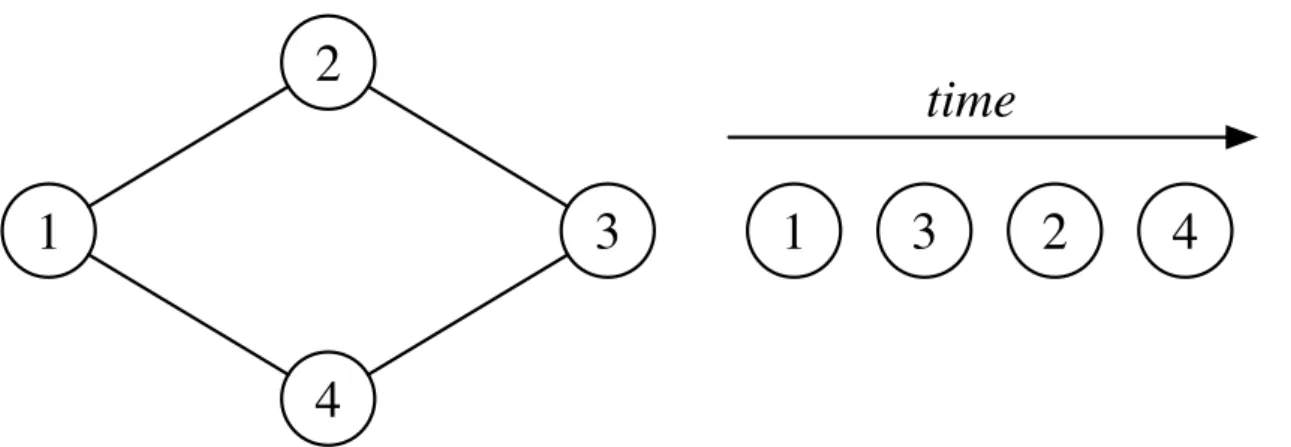
Clearly, when working with graph streams it is important to consider not only the graph elements (data), but also the order in which elements appear in a stream. Throughout this thesis, we consider the following commonplace orderings:
• Random ordering is computed by randomly permuting the existing ordering of a graph’s elements.
• Breadth-firstordering is computed by performing a bread-first traversal across the connected components of a graph. If a graph contains several connected components then these are selected in random order.
• Depth-first ordering is computed by performing a depth-first traversal across the connected components of a graph. Again, if a graph contains several such components, they are selected in random order.
One more important ordering to consider, particularly for a dynamic graph or a static snapshot of a dynamic graph, is the order in which its elements are created. We refer to this ordering as stochastic. Unfortunately, the information necessary to derive a stochastic ordering is not available for most publicly accessible datasets. There-fore, throughout this work we consider random ordering to be an imperfect proxy for stochastic as many graphs may be viewed as growing at least pseudo-randomly.
2.2
Graph operations
The various algorithms and other operations which may be executed over a graph can be broadly separated into one of two previously mentioned (Ch. 1) categories: offline analytical operations, and online data-management operations.
Offline analytical operations are often designed in a vertex-centric fashion and executed using bulk synchronous parallel (BSP) systems, such as Google’s Pregel [75]. In such BSP systems a graph operation is performed in a number of supersteps.
These operations are expressed as functions executed for each vertex, where the ver-tex contains information about itself and its neighbours. At the start of each system superstep, a vertex will receive messages sent from its neighbours during the previous superstep. The operation’s function will then execute, updating the vertex’s stored information and sending messages on to its neighbours. Additionally, during a super-step a vertex may vote to halt, rendering itself inactive. When all vertices in a graph are inactive the operation terminates.
As messages may be serialised and supersteps between partitions synchronised, these operations can execute over distributed graphs. The scalability and the relative ease of programming has made this vertex-centric pattern popular for graph processing systems [78].
There are many examples of offline analytical operations besides the PageRank al-gorithm [75] previously mentioned (Ch. 1). These include, e.g, computing minimum spanning trees [41] or graph matching algorithms [2], which derive sub-graphs con-taining only those edges not adjacent to one another and are commonly used in graph partitioners.
Three common features shared by the majority of such operations is that they a) re-quire the entire graph as input; b) take on the order of minutes to hours to complete; and c) are typically executed as one-off events or at large regular intervals (e.g. weeks). This is distinct from Online data-management operations, which typically com-plete on the order of milliseconds to seconds, consider only a very small subset of a graph and are executed continuously in large numbers.
Online operations are typically executed in systems with soft real-time constraints like graph database management systems (GDBMS) such as Neo4j [86]. Pattern matching queries, which we highlight earlier (Ch. 1), are one of the most common examples.
We consider a pattern matching query as defined in terms of sub-graph isomor-phism. Given a pattern graph q = (Vq, Eq) and a host graph G , a query should
return R: a set of sub-graphs of in G. For each returned sub-graph Ri = (VRi, ERi) there should exist a bijective function f such that: a) for every vertex v ∈ VRi, there exists a corresponding vertex f(v)∈ Vq; b) for every edge (v1, v2)∈ ERi, there exists a corresponding edge (f(v1), f(v2)) ∈ Eq; and c) for every vertex v ∈ Ri, the labels
match those of the corresponding vertices inq,l(v) =l(f(v)). As an example, consider Figure 2.1, which presents a host graph G, along with three queries (pattern graphs) q1, q2 andq3. Given the query q2, a result R is returned, containing two sub-graphs
{(1,2),(2,3)} and {(6,2),(2,3)} inG.
Although pattern matching queries may be described in terms of sub-graph isomor-phism, they are rarely implemented solely in those terms as the problem is known to be NP-Complete [43] and practical verification algorithms [79, 119] are expen-sive [99]. Instead modern pattern matching query engines adopt what is known as a filter-verify approach [32, 49, 86]. In the filter step, a graph index structure [60] to look up candidate vertices or sub-graphs, which may form part or all of a pattern match. Subsequently, in the verify step, the candidates and their local neighbourhoods are traversed, edge by edge, to detect any exact matches. Intuitively, the number of traversals which occur when executing a pattern matching query depend upon the number of candidates returned by a filter step and the average degree of the graph around each candidate.
B
A
1 2 3 4 5 6 7 8 a b c d b a d cG
Q
( q1:30%, q2:60%, q3:10% )q
3q
1q
2 a b b a a b c a b c d a bFigure 2.1: Example graph G with query workloadQ
Throughout this work we consider partitioning strategies for large graphs which ac-count for particular workloads of the above pattern matching queries. Formally, we consider a query workloadas a simple set of tuplesQ={(q1, n1). . .(qh, nh)}, where
ni is the relative frequency of each queryqi in Q.
Note that in this work we do not consider pattern matching queries as defined in terms of graphhomomorphism[32]. This is primarily because homomorphism does not imply an exact match between a pattern graph q and a host graph G, but also because the same choice (i.e. opting for isomorphism) is taken by many widely used graph query languages [32,40, 49].
Furthermore, for simplicity, we do not consider queries which perform negative pattern matching, i.e. vertex a must be adjacent to vertex b (a−b), but not c. However, all techniques presented throughout this thesis naturally apply to queries which include negative matches because the process of executing them is identical to that of executing queries with only positive matches. Consider again q2 from Fig. 2.1: to verify whether
the vertex 2 does, or does not have a clabelled neighbour, an execution engine must still traverse all neighbours of vertex 2.
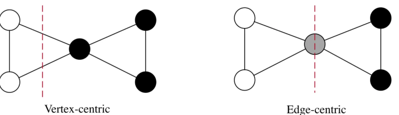
Vertex-centric
Edge-centric
Figure 2.2: Vertex vs Edge centric partitionings
2.3
Graph partitions
A k-way graph partitioning Pk(G) may be thought of as a view over a graph G,
wherein G is separated into a set of k sub-graphs. These graph partitionings are typically defined in one of two ways: vertex-centric or edge-centric.
A vertex-centric graph partitioning is defined as a disjoint family of sets of vertices Pk(G) = {V1, V2, . . . , Vk}. Each set Vi, together with its edges Ei (where ei ∈ Ei,
ei = (vi, vj), and vi, vj ⊆ Vi), is referred to as a partition Si. A partition forms a
proper sub-graph of G such thatSi = (Vi, Ei),Vi ⊆V and Ei ⊆E.
An edge-centric partitioning is similar, though defined as a disjoint family of sets of edges. Note that, in a vertex-centric partitioning2, vertices are unique to single
partitions whilst edges may be shared between two. Meanwhile, in an edge-centric partitioning, edges are unique whilst vertices may be shared between two or more partitions. Figure 2.2 provides a simple example of the difference between these two definitions.
The focus of this thesis is largely upon producing and improving those partitions which are vertex-centric.
2.4
Partitioning Quality and Objective Functions
In order to improve a graph partitioning, some consistent notion of partitioning quality is needed. Existing graph partitioners usually define this quality as one of several objective functions, i.e. some measure, calculated over an entire graph, which must be maximised or minimised.
The most common such measure is the previously mentionedmin. edge-cut (Sec. 1.2). Edge-cut is the number of edges which connect vertices in different partitions, formally: |Ecut| where e ∈ Ecut, e = (vi, vj), vi ∈ VA, vj ∈ VB and A 6= B. By minimising
the number of these inter-partition edges, systems somewhat reduce the network communication cost for a broad range of analyses, including many BSP operations and sub-graph pattern matching. Besides min. edge-cut, there are other metrics which may be used as objective functions for graph partitioners, including communication volume [76] and partition stability [24].
The communication volume of a vertex v refers to the number of distinct partitions adjacent to v, i.e. the number of partitions which contain neighbours of v but not
v itself. Communication volume partitioners minimise this metric for all the vertices v ∈V. This is similar to, but distinct from min. edge-cut partitioners: communication volume does not account for multiple edges between a vertex v and neighbours in a single partition. Communication volume partitioners have become increasingly popular for application to graphs over which min. edge-cut systems do not achieve good results, such as power-law graphs [76].
Partiton stability, first introduced by Delvenne et al. [24], is another measure of parti-tioning quality, defined in terms of network flow and random walks over a graph. The full definition of stability is left “in situ” in chapter 4, where it is required for context. Note that, by default, the measures above are not able capture the quality of a graph partitioningwith respect to a specific query workload. As a result they are unsuitable, both as objective functions for the techniques we present in this work and as a means by which to evaluate their impact.
Some measures may be modified, making themworkload-sensitive. Indeed, we propose a modified version of stability for this purpose (Sec. 4.2.2). Technically, if graph edges
are given weights corresponding to the frequency with which they are traversed by a query workload, then even min. edge-cut 3 partitionings are high quality with respect
to that workload. However, in an online system such modified metrics are expensive to calculate and impractical to update [55].
Regardless of the objective functions they employ, when evaluating the graph parti-tioning quality achieved by different algorithms, throughout this thesis we primarily consider the number of inter-partition traversals (ipt) which occur when executing a given workload Q over Pk(G). The reasons for this are twofold. Firstly, as we have
argued (Sec. 1.2), lowipt is equivalent to the true goal of graph partitioners in the con-text of data processing systems: reduced network latency 4. Secondly, unlike network
latency, ipt is a scale-free measure, independent of complex implementation details.
2.5
Partitioning Hardness
Note that, in addition to the metrics above, quality graph partitionings must be ap-proximately balanced 5. In the absence of a balance requirement, optimising for
quality metrics leads to work being distributed unevenly between partitions (and phys-ical hardware), which is inefficient. As a pathologphys-ical example, consider that a single partition containing all vertices and edges (i.e. an unpartitioned graph) is guaranteed not to cut any edges an is therefore optimal w.r.t imbalanced min. edge-cut. k-way balanced graph partitioning, as it is formally called, is known to be NP-Hard. Andreev and Racke [3] demonstrate that, if perfect partition balance is required, there exists no constant-time approximation for partitioning general graphs. They also present an algorithm which is able to offer an improved approximation of O(log2n) in the event that the balance constraint is relaxed, e.g. one partition is permitted to be 30% larger than another. However, this approximation, along with others like it [13] is too slow and expensive to be used for large graphs.
3Nowmin. edge-weight-cut
4Assuming, for simplicity, a homogeneous network and a consistent number of network packets
per traversal.
3
Related work
Contents
3.1 Local graph re-partitioners . . . 23
3.2 Global graph partitioners . . . 26
3.2.1 Spectral techniques . . . 27 3.2.2 Diffusions techniques . . . 28 3.2.3 Multilevel application . . . 29
3.3 Distributed graph partitioners . . . 32
3.4 Streaming graph partitioning . . . 34
3.4.1 Re-streaming . . . 36
3.5 Workload sensitive partitioning . . . 38
3.5.1 Offline workloads . . . 39 3.5.2 Online workloads . . . 40 3.5.3 Replication systems . . . 42
3.6 Comparing partitioner systems . . . 44
3.6.1 System properties . . . 45 3.6.2 Suitability of existing systems to online workload-sensitive
Summary
This chapter seeks to provide context for the contributions presented in our thesis by examining both the relevant background material and more recent related works.
k-way balanced graph partitioningis clearly of practical importance to any appli-cation with large amounts of graph structured data. As a result, despite the fact that the problem is known to be NP-Hard [3] and available approximation algo-rithms too expensive [13], various practical solutions have been proposed using heuris-tics [18, 52, 58, 76,90, 110, 117, 125].
In the sections that follow we survey these partitioning solutions and assign them to one of five potentially overlapping categories: Local (Sec. 3.1), Global (Sec. 3.2), Distributed (Sec. 3.3), Streaming (Sec. 3.4) and Workload-sensitive (Sec. 3.5). Graph partitioning has been the subject of significant research over many years, which we do not attempt to comprehensively review. Instead, in this chapter we highlight recent, relevant or fundamental results. Particularly close attention is paid to solutions which are either well suited to online use1, or workload-sensitive, as these may partially address the motivations for this work (Ch. 1). We refer the reader to [5, 12, 13, 106] for further general material.
Finally, in section (Sec. 3.6), we identify eight key properties for graph partition-ers, particularly those which are workload-sensitive. These properties are used as a framework for comparing the graph partitioners presented throughout the chapter, highlighting deficiencies in existing research and providing context for our own efforts. This framework will also be used to evaluate techniques presented in later chapters (Ch. 4 and 5).
3.1
Local graph re-partitioners
The category of local graph partitioners includes any partitioner which makes use of local search, which is also known as iterative vertex swapping or local refinement. Simply put, local search aims to improve an existing graph partitioning by swapping
vertices between partitions in order to minimise some objection function, usually min. edge cut. Local graph partitioners vary in how they select which vertices to swap and which partitions they will consider sending vertices between (e.g. adjacent partitions, or highly imbalanced partitions).
In their work to reduce the number of object references between memory pages during program execution, Kernighan and Lin [61] propose the classic example of a local search algorithm. Indeed perhaps the first example of a graph partitioner in general. Their key intuition was as follows: given two partitions forming halves of a balanced graph bisection P2(G) = {V1, V2}, there exist subsets of vertices A ⊂ V1, B ⊂ V2
which may be swapped between partitions to produce an arrangement that is globally optimal for some objective function (usually min. edge-cut).
The Kernighan-Lin algorithm (KL) operates in iterations, selecting vertex sets to swap which will result in the greatest improvement (which we call objective function gain, or simply gain). Within each iteration, the algorithm considers every vertex vi from
a partition (say V1), then calculates the potential gain when swapping vi with each
vertex vj from partition V2. The pair (vi, vj) with the highest gain is marked for
swapping (i.e. vi, vj are added to A, B respectively) and the next vertex in V1 \v1
is considered with each vertex in V2 \v2. Note that when considering swapping the
neighbours of vertices already marked in this iteration, the potential objective gain for those neighbours is calculated as if marked verticeshave already been swapped. When every vertex has been considered, the sets A, B are swapped between partitions and the next iteration may begin. Iterations continue until the total gain for all suggested swaps is ≤0.
There are two main issues with the KL algorithm as a graph partitioner. The first is that it is limited to improving the partitioning quality of graph bisections, rather than k-way partitionings. The second is that it is highly expensive, with a single iteration of the algorithm having the complexity O(n2logn), remembering that n=|V|.
In order to address such issues with theKLalgorithm, several improvements have been proposed. Perhaps most significantly, Fiduccia and Mattheyses [33] present a modified
algorithm (KL/FM) which is significantly less expensive. The iteration complexity for
KL/FM is O(m), nothing thatm =|E| and that the upper bound 2form is (n−1)2.
There are two major differences between the KL/FM andKL algorithms. Firstly, the vertex swapping between bisections is asymmetric, i.e. vertices are marked for transfer individually, rather than as a pair with a vertex from the other partition. This means that for each vertex considered for swapping, it is not necessary to consider every vertex from the other partition. Secondly, Fiduccia and Mattheyses use a datastructure called a bucket queue [80] for efficiently updating neighbour objective function gain after marking vertices for swapping.
Despite the improvement that the KL/FM algorithm represents, it shares KL’s orig-inal limitation of being application only to graph bisections. However there are ex-tensions of local search techniques which generalise to improving k-way partition-ings [58, 98, 132]. Notably, Karypis and Kumar [58]propose an algorithm they call Greedy Refinement (GR) as part of their work on the well know global partitioner METIS, which we discuss shortly.
For efficiency, GR moves only boundary vertices 3 between partitions, considering all such vertices in random order during each iteration. For each vertexv,GR orders the partitions to which v is adjacent by the potential gain of moving v to them, subject to some balance constraints. If a move does not satisfy chosen balance constraints, then progressively less beneficial destination partitions are considered. Once a destination partition has been chosen, the move is immediately performed and the next random vertex considered. An iteration of GR terminates when more than some threshold number of vertex moves have been performed without any positive objective function gain as a result.
Unfortunately, despite some ability to climb out of local optimisation minima, the quality of partitionings produced by the local search algorithms above is strongly de-pendent on the quality of the initial partitionings they receive. They remain important to consider however, for two reasons. Firstly, they are often integrated as part of a
2In the rare case of a strongly connected simple graph with an edge from each vertex to every
other vertex.
global graph partitioner [51, 58, 101] such as with Greedy Refinement and the afore-mentioned METIS [58]. Secondly, as the name local search implies, the information required for each vertex migration is local to that vertex. This allows asymmetric methods to perform very little or no global coordination between partitions. As a re-sult, such methods are effectively applied in distributed settings [98, 120, 131], where inter-partition coordination is costly.
3.2
Global graph partitioners
In general, global graph partitioners [9,26,28, 29, 50,51,58,64,82, 90, 102] refers to those partitioners which, unlike their local counterparts, take an entire unpartitioned graph as input. By default, such partitioners are also executed within the confines of a single machine.
They are the most commonly used family of techniques, likely due to their effectiveness: global graph partitioners produce some of the highest quality partitionings of any techniques we consider. Indeed Karypis and Kumar’s METIS [58] is considered the de-facto gold standard for partitioning quality [76]. However, it is also likely that the popularity of such techniques is at least partially due to their being relatively simple to use and available in a number of robust software packages4 5 6.
As we alluded to previously in Chapter 1, however, simple (undistributed) global graph partitioners are not without their drawbacks, particularly in an online setting. Firstly, they are highly resource intensive [120] and are typically performed ahead of offline analytical workloads. Additionally, they require an entire graph to be availablea priori
as input, and may therefore require periodic re-execution, i.e. given a dynamic graph following a series of graph updates, which is impractical online [55].
Secondly, like local graph partitioners, the vast majority of global partitioning tech-niques [33, 58, 90, 102, 110, 117] optimise for the min. edge cut objective function. This renders them workload-agnostic: assuming uniform and constant usage of a graph by a workload. As a result the partitionings they produce, whilst effective at reducing
4The METIS [58] family of graph partitioning software:
http://bit.ly/1tqUcSQ
5The Scotch [90] graph partitioning software:
http://bit.ly/2r2mbfI
6The KaHiP [102] graph partitioning software:
the runtime of distributed analytical jobs (e.g. Pagerank), are sub-optimal for other types of workload, such as sub-graph pattern matching queries, which are common in an online graph data-management setting.
Note that although global graph partitioners are broadly similar in terms of advantages, disadvantages and behaviour, they may differ significantly in the method of their implementation. For example, some systems [26,82,90] use the natural representation of a graph as a network, and derive partitions in terms of breadth-first traversals and diffusion. Other systems [9, 28, 29, 51], known as spectral partitioners, treat graphs as matrices and derive partitions using linear algebra.
Finally, some global partitioning systems [50, 58, 64, 90, 102] apply an existing tech-nique (spectral, diffusion-based or otherwise), but over compressed versions of a graph. These systems, which are calledmultilevel, are arguably the most effective global graph partitioners in terms of performance, scalability and partitioning quality.
3.2.1
Spectral techniques
Spectral graph partitioning was first proposed by Donath and Hoffman [29] for com-puting bisections of a graph G with respect to min. edge-cut. Firstly the Laplacian matrix LG of G is computed by subtractingG’s adjacency matrix AG from its degree
matrix DG, LG = DG −AG. Secondly, the eigenvector associated with the second
smallest eigenvalue of LG is computed. The algorithm relies upon the intuition that
this eigenvector, called the Fiedler vector [34], contains an integer value for each vertex, which corresponds to its connectedness in the graph. Using this value as an order-ing, the algorithm then divides the vertices of G around the median, into two sets of equal size. These sets represent a bisection which is good with respect to min. edge-cut. Note that this algorithm generalises to producing k-way partitionings of graphs through recursively bisecting generated partitions7. All other spectral partitioning
techniques [9,28, 51] extend this core algorithm.
These extensions usually aim to improve performance as, in practice, the Fielder vector is approximated using Lanczos algorithm [67] which is highly computationally expen-sive for large graphs. For instance, Hendrickson and Leland [51] propose a method
for computing graph partitionings wherek > 2without recursive application , thereby avoiding computing the Fiedler vector more than once. Furthermore, Barnard and Simon [9] propose a multilevel spectral method. Whilst the algorithm is structurally similar to those we discuss in section 3.2.3, Barnard and Simon do not compute and refine a graph partitioning over compressed versions of a graph. Instead, they compute and refine an approximation of a Fiedler vector over compressed versions of a given graph, thereby substantially reducing its computational cost. This Fiedler vector is subsequently used to compute a bisection over the uncompressed graph.
3.2.2
Diffusions techniques
Besides spectral techniques, there are a number of global graph partitioners which employ random walks or breadth-first traversals in order to derive partitions [26, 82, 90]. These systems are broadly referred to as Diffusion-based and implement some variation on the following simple algorithm:
Firstly, for ak-way partitioning, k seed nodes are selected, evenly distributed out a graph’s structure. Secondly, random walks or traversals are performed through-out the graph, originating from these seeds. Each vertex may only be traversed once. Once all vertices have been traversed, each vertex belongs to the same partition as its traversal’s seed. This procedure is often employed iteratively, with new seeds being selected each round [26, 82]. Diekmann et al. [26] were the first to propose this mod-ification, referring to is as the Bubble framework. Meyerhenke et al. [82] extend the Bubble framework, generalising it to graphs with variable edge weights and improving its performance by introducing a random walk mechanism which only operates over small (local) areas of a graph.
Whilst Diffusion and traversal based partitioning techniques can yield high quality results, they are also somewhat computationally intensive. Variants of the Bubble framework have a worst case complexity of O(km), wheremis equal to the number of vertices in a graph and k the desired number of partitions. Additionally, naive imple-mentations of the Bubble framework can lead to highly imbalanced partitions [103], though this limitation is usually addressed through the use of additional heuristics, these may add to the overall computational complexity of a scheme.
Pellegrini et al. also employ diffusion-based techniques in their popular graph parti-tioning tool Scotch [90]. However, Scotch is an example of the multilevel partitioners we discuss in the following section. In other words, in order to ameliorate the com-plexity of diffusion-based partitioning, they only apply their technique to compressed versions of a graph and even then, only to vertices near predicted partition boundaries.
3.2.3
Multilevel application
As mentioned at the start of this section, some of the most effective global graph partitioning systems are known as multilevel [50, 58, 64, 90, 102]. Proposed in its current form by Hendrickson and Leland [50], multilevel partitioning works in three stages: coarsening, partitioning and uncoarsening.
The Coarsening stage: a succession of recursively compressed graphs is computed, tracking exactly how the graph was compressed at each step.
The Partitioning stage: the coarsening stage continues until the most compressed form of the graph is small enough that an initial partitioning may be trivially produced using an existing technique (e.g. spectral partitioning).
The Uncoarsening stage: using the knowledge of how each compressed graph was produced from the previous one, the initial partitioning is then “projected” back onto the original graph, using a local technique (e.g. KL/FM [33]) to improve the partitioning after each step. Figure 3.1 presents an example of multilevel partitioning over a small graph.
The various multilevel techniques which exist differ in how they implement the above three stages. Consider the canonical example of a multilevel partitioner: the afore-mentioned METIS [58].
In the coarsening stage METIS compresses a graph G by computing maximal egde matchings [50]8. An edge matching is defined as a set of edgesE
M fromG, such that
no two edges in EM are incident upon the same vertex. Given such a matching, a
Trivial partitioning Com pre ss Uncom pre ss
Figure 3.1: The partitioning pattern common to multilevel apparoaches. Inspired by similar figures in [58, 102]
single level of compressed graph is computed by combining vertices connected by an edge e∈EM, treating each pair as a single “multi” vertex. Compression is performed
using these matchings rather than, for example, arbitrarily combining vertices as it prevents any one “multi” vertex from containing many more elements than another. As a result, a balanced partitioning of the compressed graph will correspond to a balanced partitioning of the original graph.
Next, when computing an initial partitioning for the compressed graph GM, METIS
uses a technique based upon spectral recursive bisection. Finally, in the uncoarsening stage of partitioning, METIS uses the Greedy Refinement local algorithm (Sec. 3.1) to move “multi” vertices between partitions, improving the partitioning after each step of match/combine compression has been reversed.
On the other hand, consider alternative multilevel partitioners [64, 102]. Korosec and Silc propose MACA [64], which uses an ant-colony optimisation technique for both initially partitioning the most compressed graph, and for improving the partitioning after each step of the uncoarsening stage. This is interesting because ant-colony
opti-misation techniques are highly parallelisable; a fact Tashkova et al. exploit with their work in Distributed MACA [112] (DMACA). Meanwhile, Sanders and Schulz [102] propose an edge rating function which prioritises edges which are close w.r.t algebraic distance [15]9 when computing edge matchings in the coarsening phase. As a result of
this edge rating function, good partitionings of compressed graphs correspond to good partitionings of their uncompressed counterparts, even more closely than with other matching techniques.
In general, the three key advantages to a multilevel approach to global graph parti-tioning may be summarised as follows: Firstly, as matchings and other forms of graph compression are relatively inexpensive, it is possible to compress large graphs before applying an initial partitioning technique which is highly effective, but would be be impractically expensive at the graph’s original scale. Secondly, the local partitioning techniques applied during the uncoarsening stage will perform well, given that the movement of a vertex in the compressed graph corresponds to the movement of sev-eral vertices in the original graph and that each compressed graph . Finally, due to the initial partitioning and repeated improvements, the input to each step of uncoars-ening will be of high quality; as mentioned (Sec. 3.1) this significantly increases the effectiveness of local partitioning techniques performing the improving.
As a result of these advantages, multilevel partitioners are the most performant and effective of all global graph partitioners. Despite this, they still share many of the disadvantages, such as optimising for an objective function and requiring an entire graph as input. This means they too are not suited for graphs which may grow, or be subject to a changing workload; i.e. they are unsuitable for application to an online graph data-management setting. Most importantly, however, the scalability of such undistributed multilevel partitioners remains fundamentally limited by the resources of their host hardware and so struggle to partition graphs with a more than a few tens of millions of vertices and edges [117].
9Edges which are part of strongly connected clusters in a graph will have low algebraic distance
3.3
Distributed graph partitioners
In order to scale to graphs which do not fit within the memory of a single machine, global graph partitioners (i.e. those which require the entire graph a priori) must be modified to operate when distributed: executed by multiple machines communicating via a network.
As mentioned in Chapter 1, in recent years there have been an increasing number of applications making use of such large amounts of graph data, such as social net-working [47, 122], search engines [11] and genome analysis [10, 121]. As a result, several distributed graph partitioning algorithms have been proposed, often as exten-sions to existing systems, e.g. PT-Scotch [18], ParMETIS [59] and ParHIP [83] and DMACA [112].
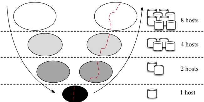
These distributed extensions [18, 59] are implemented along broadly similar lines to their single-machine counterparts. In other words, the first stage of the algorithm is to recursively coarsen/compress a graph, this time by computing a distributed maximal edge matching. Intuitively, computing whether a given inter-partition edge forms part of a matching requires coordination between the machines to which the edge’s two vertices belong. Typically, this coordination happens iteratively, with each partition sending messages to it’s neighbours, proposing and rejecting potential matched edges in rounds. To reduce the communication overhead caused by these messages, progres-sively smaller graphs are gathered (or “folded”) onto smaller numbers of machines until, at the end of the coarsening stage, the smallest graph resides on a single machine.
Once, the smallest graph is contained on a single machine, the initial partitioning stage takes place as normal. Subsequently, during the uncoarsening stage, the graph partitioning is refined using a local refinement technique to move vertices between (distributed) partitions. In addition, after each step of uncoarsening, the graph par-titioning is “unfolded” back onto a larger number of machines. Fig. 3.2 presents an example of this distributed multilevel partitioning process.
Meyerhenke et al’s recent ParHIP [83] follows a similar pattern, though employs a novel parallel label-propagation based graph clustering technique to coarsen the input graph, instead of computing an edge matching. This label-propagation technique is
8 hosts
4 hosts
2 hosts
1 host
Figure 3.2: Example of “folding” in distributed mulilevel graph partitioners.highly effective, producing significantly smaller graphs at the coarsest level than other edge matching techniques, and allowing ParHIP to partition larger graphs than is possible with, e.g. ParMETIS.
Another interesting example of a distributed graph partitioner which uses label-propagation is JA-BE-JA [98]. JA-BE-JA is actually an example of a local-search technique (Sec. 3.1), using vertex labels to denote partition assignments, and iteratively swapping labels between neighbouring vertices. Additionally, JA-BE-JA uses simulated anneal-ing to escape local optimisation minima better than other local search techniques.
Finally, Margo and Seltzer’s work on Sheep [76] is worthy of consideration. The Sheep algorithm efficiently creates an elimination tree [92] from a distributed graph using a map-reduce procedure, then partitions the tree and subsequently translates it into a partitioning of the original graph. Unlike the other distributed partitioners we consider, which optimise for min. edge-cut, Sheep optimises for the min. communication volume objective function. In other words, it minimises the number of different partitions in which a given vertexvhas neighbours. This metric has been shown to be more effective than min. edge-cut for producing partitionings of certain graphs, such as graphs whose degrees are distributed according to a power-law.
In general distributed partitioners exhibit significantly improved scalability, success-fully partitioning graphs with billions of edges [83]. Furthermore, because such
algo-rithms require input graphs to be spread between host machines, they are theoretically applicable tore-partitioning a graph in situ, unlike their single-machine counterparts.
Despite addressing the scalability concerns of global graph partitioners, the distributed systems above are not without their drawbacks, however. Principle among these is communication cost: all of the above systems incur significant communication over-head, both when computing a new partitioning10 and when migrating vertices and
edges between partitions.
Whilst some techniques do exist to minimise the number of inter-partition vertex swaps which occur during a repartitioning [104], these inevitably trade off against the quality of the final partitioning. Additionally, such techniques have been shown to have only a limited effect [132].
As a result, despite distributed partitioners’ theoretical applicability to the task, graph analytical frameworks often employ them only as initial, highly scalable, partitioning step, rather than for repeated repartitioning [62].
Finally, note that distributed partitioners share the other drawbacks of normal global partitioners, besides scalability. In particular, they remain unsuitable for dynamically growing graphs and agnostic to changes in the workloads being applied to them.
3.4
Streaming graph partitioning
Like the distributed systems above, streaming graph partitioners [52, 87, 110, 117] have been proposed to address the scalability and performance issues of global par-titioners. The strict streaming model considers each element of a graph stream11 as soon as it arrives, efficiently assigning it to a partition. Additionally, streaming parti-tioners do not perform any refinement of portions of the graph already considered and partitioned. In other words, they will not employ local refinement techniques to move vertices to other partitions, nor perform any sort of global introspection such as in spectral partitioning. This model has two key advantages. Firstly, the memory usage of streaming partitioners is both low and independent of the size of the graph being
10In spite of improvements due to “folding” heuristics [18, 59]. 11This may be either vertices or edges.
partitioned, allowing them to scale to to very large graphs (e.g. billions of elements). Secondly, although graph streams are often created by reading static data serially from disk, streaming partitioners may trivially be applied to dynamically growing graphs by treating each new edge or update as an element in the stream. This is in stark contrast to the mentioned difficulties with applying distributed partitioners to such graphs.
The canonical examples of streaming graph partitioners are Linear Deterministic Greedy (LDG) [110] and Fennel [117], which both make partition assignment decisions on the basis of inexpensive heuristics considering the local neighbourhood of each vertex 12
at the time it arrives. LDG was proposed by Stanton and Kliot in a survey of vari-ous streaming graph partitioning heuristics, where it was the most effective technique considered. It assigns vertices to the partitions where they have the most existing neighbours, but penalises that number of neighbours for each partition by how full it is, maintaining balance. Later, Tsourakakis et al. propose Fennel, which interpolates between the LDG and another heuristic [95], which amounts to assigning vertices to the partitions where they have the fewest non-neighbours. Fennel produces partition-ings of higher quality than LDG w.r.t. min. edge-cut, in similar runtime, though at the cost of slightly worse partitioning balance.
Despite offering unlimited scalability and up to an order of magnitude speedup vs global and distributed techniques [117], streaming partitioners have their drawbacks as well. By relying upon the available local neighbourhood information for a vertexvat the time v is added to the graph stream, such techniques render themselves sensitive to the graph stream’s ordering. For example, consider one of the common stream orderings outlined in chapter 2.1.1,breadth-first (BFS). Given a BFS ordering, a graph stream maintains a high degree of locality: vertices which are connected will appear close together within the stream. As a result, for each new vertex v which arrives in a BFS stream, the partitioner has likely already placed many of its neighbours and can make an effective decision about where to placev such that it is in the same partitions as the largest number of them.

![Figure 3.1: The partitioning pattern common to multilevel apparoaches. Inspired by similar figures in [58, 102]](https://thumb-us.123doks.com/thumbv2/123dok_us/1985214.2794823/44.892.111.693.121.554/figure-partitioning-pattern-multilevel-apparoaches-inspired-similar-figures.webp)
![Table 3.1: Properties of Graph partitioners System S D SC DY RF WS OW TX KL/FM [33] Y P Y Spectral [9, 28, 51] Y DMACA [112] Y Y PT-Scotch [18] Y Y Y ParMETIS [59] Y Y Y ParHiP [83] Y Y Y Sheep [76] Y Y Y LDG [110] Y Y Y Y Fennel [117] Y Y Y Y Nishimura et](https://thumb-us.123doks.com/thumbv2/123dok_us/1985214.2794823/61.892.221.795.159.610/properties-partitioners-spectral-scotch-parmetis-parhip-fennel-nishimura.webp)