Structural Vector Autoregressions with Markov Switching

Full text

(1)DEPARTMENT OF ECONOMICS. EUI Working Papers ECO 2009/06 DEPARTMENT OF ECONOMICS. Structural Vector Autoregressions with Markov Switching. Markku Lanne, Helmut Lütkepohl and Katarzyna Maciejowska.

(2)

(3) EUROPEAN UNIVERSITY INSTITUTE, FLORENCE. DEPARTMENT OF ECONOMICS. Structural Vector Autoregressions with Markov Switching MARKKU LANNE, HELMUT LÜTKEPOHL and KATARZYNA MACIEJOWSKA. EUI Working Paper ECO 2009/06.

(4) This text may be downloaded for personal research purposes only. Any additional reproduction for other purposes, whether in hard copy or electronically, requires the consent of the author(s), editor(s). If cited or quoted, reference should be made to the full name of the author(s), editor(s), the title, the working paper or other series, the year, and the publisher. The author(s)/editor(s) should inform the Economics Department of the EUI if the paper is to be published elsewhere, and should also assume responsibility for any consequent obligation(s). ISSN 1725-6704. © 2009 Markku Lanne, Helmut Lütkepohl and Katarzyna Maciejowska Printed in Italy European University Institute Badia Fiesolana I – 50014 San Domenico di Fiesole (FI) Italy www.eui.eu cadmus.eui.eu.

(5) January 26, 2009. Structural Vector Autoregressions with Markov Switching1 Markku Lanne Department of Economics, P.O. Box 17 (Arkadiankatu 7), FI-00014 University of Helsinki, FINLAND email: [email protected]. Helmut Lütkepohl Department of Economics, European University Institute, Via della Piazzola 43, I-50133 Firenze, ITALY email: [email protected]. Katarzyna Maciejowska Department of Economics, European University Institute, Via della Piazzola 43, I-50133 Firenze, ITALY email: [email protected] Abstract. It is argued that in structural vector autoregressive (SVAR) analysis a Markov regime switching (MS) property can be exploited to identify shocks if the reduced form error covariance matrix varies across regimes. The model setup is formulated and discussed and it is shown how it can be used to test restrictions which are just-identifying in a standard structural vector autoregressive analysis. The approach is illustrated by two SVAR examples which have been reported in the literature and which have features which can be accommodated by the MS structure. Key Words: Cointegration, Markov regime switching model, vector error correction model, structural vector autoregression, mixed normal distribution JEL classification: C32. 1. We thank Pentti Saikkonen for helpful discussions about the model setup and the associated inference procedures. The research of the first author was supported by the Academy of Finland and the Yrjö Jahnsson Foundation. This paper replaces an earlier version which was circulated under the title Stock Prices and Economic Fluctuations: A Markov Switching Structural Vector Autoregressive Analysis by the first two authors..

(6) 1. Introduction. In structural vector autoregressive (SVAR) modelling a major problem is to find convincingly identified shocks which are informative about the actual reactions of a set of variables to unexpected exogenous innovations. Although economic theories and models often provide some information which can be used for identification, this is not always sufficient to fully identify the shocks of interest. Different cures for this problem have been proposed over the years. In the earlier VAR literature a triangular orthogonalization of the shocks which results in a recursive structure was quite popular (e.g, Sims (1980)). This kind of identification was often based on some ad hoc reasoning and sometimes it was proposed to try different orderings which would result in different recursive structures and check the robustness of the main results (Amisano and Giannini (1997), Lütkepohl (2005, Section 2.3.2)). Another proposal is to identify only some of the shocks (see Christiano, Eichenbaum and Evans (1999)). This approach works well as long as there is information to identify the shocks of primary interest. Unfortunately, this is not always possible (see again Christiano et al. (1999)). Other approaches use restrictions for the long-run effects of the shocks (Blanchard and Quah (1989), King, Plosser, Stock and Watson (1991), Pagan and Pesaran (2008)), inequality restrictions (Uhlig (2005), Canova and De Nicoló (2002), Faust (1998)), Bayesian methods (Koop (1992)) or statistical properties of the data such as the residual distribution (Lanne and Lütkepohl (2009)), structural breaks or heteroskedasticity (Rigobon (2003), Lanne and Lütkepohl (2008)). In this study we will consider the latter type of identifying information. In other words, we will use specific properties of a statistical model to achieve identification. More precisely, we will consider special features of Markov regime switching (MS) models to identify structural shocks. These models were introduced by Hamilton (1989) as tools for time series econometrics. They were extended to the VAR case by Krolzig (1997) and they have been considered for SVAR analysis, e.g., by Sims and Zha (2006) and RubioRamirez, Waggoner and Zha (2005). Sims, Waggoner and Zha (2008) present Bayesian methodology for handling general versions of MS-SVAR models. They were found to be useful, for instance, in business cycle analysis. Thus, they are potentially suitable models in many situations where SVAR models have been used traditionally. In contrast to other MS-VAR studies we will argue that in these models shocks can be identified by the assumption that they are orthogonal across different regimes. Conditions will be given which ensure identification of the shocks under this assumption. A crucial condition is that the residual covariance matrices of the VAR model vary across regimes. In fact, since identification will hinge on MS in the residual covariance matrix, 1.

(7) we will focus on a model where the other parameters are constant across regimes. Such models were found to be particularly useful in applications reported by Sims and Zha (2006) and Sims et al. (2008). An important advantage of our approach is that some crucial assumptions necessary for the identification of the shocks can be checked with statistical methods. We will also discuss an extension of the setup to systems with integrated and cointegrated variables. In that case we will consider vector error correction models (VECMs) which makes it easy to accommodate longrun restrictions for the effects of the shocks in a way proposed by King et al. (1991) and others. To illustrate our approach we apply it to two examples from Lanne and Lütkepohl (2009). The first one considers a stationary system consisting of US gross domestic product (GDP), an interest rate and stock prices. It was used previously to investigate the impact of fundamental shocks on stock prices. The second example is based on a VECM and analyzes the relation between European and US interest rates. The paper is structured as follows. In the next section our model setup is presented, identification is discussed and the associated estimation strategy is considered. In Section 3 the empirical applications are presented and conclusions are provided in Section 4. A theoretical result regarding matrix decompositions is given in the Appendix.. 2 2.1. The Model General Setup. We consider a K-dimensional reduced form VAR(p) model of the type yt = Ddt + A1 yt−1 + · · · + Ap yt−p + ut ,. (2.1). where yt = (y1t , . . . , yKt )0 is a K-dimensional vector of observable time series variables, dt is a deterministic term with coefficient matrix D, the Aj ’s (j = 1, . . . , p) are (K × K) coefficient matrices and ut is a K-dimensional white noise error term with mean zero and positive definite covariance matrix Σu , that is, ut ∼ (0, Σu ). If some of the variables are cointegrated, the VECM form may be more convenient, ∗ + Γ1 ∆yt−1 + · · · + Γp−1 ∆yt−p+1 + ut , ∆yt = D∗ d∗t + αβ 0 yt−1. (2.2). where ∆ denotes the differencing operator, defined such that ∆yt = yt − yt−1 , Γj = −(Aj+1 + · · · + Ap ) (j = 1, . . . , p − 1) are (K × K) coefficient matrices, 2.

(8) α is a (K × r) loading matrix of rank r, β is the (K ∗ × r) cointegration matrix which may include parameters associated with deterministic terms and ∗ yt−1 is yt−1 augmented by deterministic terms in the cointegration relations. The rank r is the cointegrating rank of the system. The term d∗t represents unrestricted deterministic components and its parameter matrix is denoted by D∗ . In the standard SVAR approach a transformation of the reduced form residuals ut is used to obtain the structural shocks, say εt . A transformation matrix B is chosen such that εt = B −1 ut ∼ (0, IK ) has identity covariance matrix, that is, the structural shocks are assumed to be orthogonal and typically their variances are normalized to one. Hence, Σu = BB 0 . To obtain identified, unique structural shocks, some restrictions have to be imposed on B. Often zero restrictions or long-run constraints are used in this context. A zero restriction on B implies that a certain shock does not have an instantaneous effect on one of the variables whereas long-run restrictions exclude permanent effects of shocks on some or all of the variables. Specific examples will be considered in our applications in Section 3. It is also straightforward to extend the models considered so far to allow for restrictions to be placed on the instantaneous relations of the variables rather than the shocks. This is most easily done in the context of the so-called AB model, the VAR version of which has the form Ayt = Ddt + A1 yt−1 + · · · + Ap yt−p + Bεt .. (2.3). For this model the reduced form covariance matrix is Σu = A−1 BB 0 A−10 . More restrictions are needed to identify both A and B. Often one of the two matrices is the identity matrix, however, and it is just a matter of convenience to place the restrictions on the other matrix. Notice that, although normality of the ut ’s is often assumed for convenience, such an assumption is usually not backed by theoretical considerations nor is it necessarily required for asymptotic inference. Moreover, VAR residuals are often found to be nonnormal in applied work. In the following we will specify a Markov switching structure on the residuals which implies a more general distribution class for the ut ’s and we will discuss how that can be used for the identification of shocks.. 2.2. Markov Regime Switching Residuals. We assume that the distribution of the error term ut depends on a Markov process st . More precisely, it is assumed that st (t = 0, ±1, ±2, . . . ) is a discrete Markov process with two different regimes, 0 and 1. We focus on a 3.

(9) two regime case here for convenience to simplify the following notation and discussion. An extension to more than two regimes is straightforward. The case of two regimes only is also considered in the applications in Section 3 and is therefore preferable here to simplify the discussion of the identification of shocks. The transition probabilities are pij = Pr(st = j|st−1 = i),. i, j = 0, 1.. The conditional distribution of ut given st is assumed to be normal, ut |st ∼ N (0, Σst ).. (2.4). Although the conditional normality assumption is made for convenience, it should be clear that it opens up a much wider class of distributions than just the unconditional normal. We will discuss this issue further below. The distributional assumption will be used for setting up the likelihood function. If normality of the conditional distribution does not hold, the estimators will only be pseudo maximum likelihood (ML) estimators. The normality assumption in (2.4) is not essential for our identification of shocks. Note that in our model the transition probabilities are the same in all periods. They can be conveniently summarized in the (2 × 2) transition matrix · ¸ p00 p01 P = . p10 p11 This matrix contains all necessary conditional probabilities to reconstruct the distributions of the stochastic process st . For example, the unconditional distribution of st can be derived from the conditional probabilities in P (see, e.g., Hamilton (1994, Chapter 22)). For later reference we mention that the unconditional probabilities of the states of an ergodic Markov chain are Pr(st = 0) = 1− Pr(st = 1) = (1 − p11 )/(2 − p00 − p11 ). Moreover, p10 = 1 − p00 and p01 = 1 − p11 . If p00 = p01 and p11 = p10 , the conditional distributions of the states are independent of the previous state, that is, Pr(st = j) = Pr(st = j|st−1 = 0) = Pr(st = j|st−1 = 1),. j = 0, 1.. Hence, the MS model reduces to a model with mixed normal (MN) errors, ½ N (0, Σ0 ) with probability γ = p00 , ut ∼ N (0, Σ1 ) with probability 1 − γ = p11 .. 4.

(10) In that case the transition matrix has the form · ¸ γ γ P = . 1−γ 1−γ. (2.5). Given that mixed normal distributions constitute a very large and flexible class of distributions, this shows that assuming a conditional normal distribution in (2.4) results in a very rich distribution class for the error terms. The case of mixed normal errors in the context of SVAR analysis was considered by Lanne and Lütkepohl (2009). Identification of shocks in the MS model can be achieved by the assumption that the shocks are orthogonal across regimes and only the variances of the shocks change across regimes while the impulse responses are not affected. In particular, the instantaneous effects are the same in all regimes. Note that the assumption of time invariant impulse responses throughout the sample period is common in standard SVAR analysis and, hence, not a particularly restrictive element in our setup. A well-known result of matrix algebra establishes that there exists a (K × K) matrix B such that Σ0 = BB 0 and Σ1 = BΛB 0 , where Λ = diag(λ1 , . . . , λK ) is a diagonal matrix (e.g., Lütkepohl (1996, Section 6.1.2)). From Σ0 = BB 0 and Σ1 = BΛB 0 we get a total of K(K + 1) equations which can be solved uniquely for the K 2 elements of B and the K diagonal elements of Λ under mild conditions. In the Appendix we give a result which implies that the matrix B is unique up to changes in sign if all diagonal elements of Λ are distinct and ordered in some prespecified way. For example, they may be ordered from smallest to largest or largest to smallest. The result in the Appendix is formulated in such a way so that it can be used for models with more than two regimes. For the case of two regimes the important point to note here is that our setup delivers shocks εt = B −1 ut which are orthogonal in both regimes. Since B is unique (up to sign changes), the model is in fact identified by the assumption that the shocks have to be orthogonal and the instantaneous effects are identical across regimes. Thus, any restrictions imposed on B in a conventional SVAR framework become over-identifying in our setup and, hence, can be tested against the data. The nonuniqueness of B with respect to sign in our framework is no problem for our purposes. The precise condition is that all signs in any of the columns of B can be reversed. This corresponds to considering negative shocks instead of positive ones or vice versa. Usually it will not be a problem for the analyst to decide on whether positive or negative shocks are of interest. Also, from the point of view of asymptotic inference, local identification of this kind is sufficient for the usual results to hold. Provided no sign restrictions are used, this kind of nonuniqueness of the shocks with respect 5.

(11) to sign changes is also common in standard SVAR analyses although this is not always emphasized. Rubio-Ramirez et al. (2005) also discuss identification in MS-SVAR models. However, they allow all parameters to differ across regimes. In their setup, assuming the same impulse responses in all regimes is not plausible and therefore assuming the same instantaneous effects of the shocks would be restrictive. Hence, they use alternative identification conditions. In our setup MS is confined to the error covariance matrix only and no MS is assumed in other parameters because the latter is not needed for the identification of the shocks and we try to remain as close as possible to the standard SVAR approach which assumes time invariant impulse responses for the full sample period. Allowing for MS in the residuals only means that we basically remain within a standard SVAR model. In fact, this feature of a model was diagnosed but not used for identification in Sims and Zha (2006), for example.. 2.3. Estimation. Under our assumption of conditional normality given a particular state in (2.4), maximum likelihood (ML) estimation is a plausible estimation method. If the conditional normality does not hold it will deliver pseudo ML estimators. Hence, for a 2-state MS-VAR model the parameters are estimated by maximizing the (pseudo) log likelihood function lT =. T X. log f (yt |Yt−1 ),. t=1. where Yt−1 = (y−p+1 , . . . , yt−1 ), 1 X. f (yt |Yt−1 ) =. Pr(st = j|Yt−1 )f (yt |st = j, Yt−1 ). j=0. and ¾ 1 0 −1 exp − ut Σj ut , 2 ½. −K/2. f (yt |st = j, Yt−1 ) = (2π). −1/2. det(Σj ). j = 0, 1.. Here Σ0 = BB 0 , Σ1 = BΛB 0 and the ut are the reduced form residuals. Moreover, ¸· ¸ · ¸ · Pr(st−1 = 0|Yt−1 ) Pr(st = 0|Yt−1 ) p00 p01 , = p10 p11 Pr(st−1 = 1|Yt−1 ) Pr(st = 1|Yt−1 ) 6.

(12) where Pr(st = j|Yt ) , = Pr(st = j|Yt−1 )f (yt |st = j, Yt−1 ). 1 X. Pr(st = i|Yt−1 )f (yt |st = i, Yt−1 ) ,. i=0. j = 0, 1. The optimization of lT may be done with a suitable extension of the EM algorithm described in Hamilton (1994, Chapter 22). A blockwise algorithm for computing the ML or, in a Bayesian framework, the posterior mode estimates was proposed by Sims et al. (2008) which may be more suitable for models with many free parameters, e.g., when many variables are considered and the number of regimes is larger than 2 or 3. The properties of Gaussian ML estimation in a univariate model of type (2.4) (that is, the process is white noise conditional on a given state of the Markov chain) were discussed by Francq and Roussignol (1997). Very general asymptotic estimation results for stationary processes are available in Douc, Moulines and Rydén (2004). The case of cointegrated VARs seems less well explored. If the cointegration relations are known, there is no problem because the results for stationary processes can be used. For the situation where the cointegration relations are unknown we propose to use a two-step estimation procedure. In the first step the cointegration relation is estimated by Johansen’s (1995) reduced rank regression. Then an ML estimation conditional on the first-step cointegration relation is performed. Although there is no apparent reason why this procedure should not result in estimators with standard asymptotic properties, we admit that we do not know of a formal proof if the cointegration matrix is unknown and has to be estimated. In the application in Section 3.2, where cointegrated variables are considered, assuming known cointegration relations turns out to be reasonable.. 3 3.1. Illustrations US Model. Our first example uses a small system of US macro variables from Binswanger (2004) which has also been used by Lanne and Lütkepohl (2009). The purpose of Binswanger’s analysis was to determine the impact of fundamental shocks on the stock market. The issue has been discussed previously in the literature. For example, in an SVAR analysis Rapach (2001) finds that macro shocks have an important effect on real stock prices. On the other 7.

(13) hand, Binswanger (2004) uses US data from 1983 to 2006 and concludes that real activity shocks explain only a small fraction of the real stock price variability. It is not uncommon in SVAR analyses that the specification of the shocks is essential for the outcome. We use quarterly US data for the period 1983Q1 − 2006Q3 for the three variables (gdpt , rt , spt )0 , where gdpt denotes log real gross domestic product, rt is the 3-months Treasury bill rate and spt stands for log real stock prices, as in Lanne and Lütkepohl (2009). More details on the data are given in Appendix B of the latter paper. Binswanger’s objective was to assess the importance of fundamental shocks for stock price movements. Fundamental shocks in this context are shocks which have a long-term impact on economic growth and the interest rate. Binswanger (2004) assumes that there is just one nonfundamental shock. It is specified by the requirement that it may have a long-term impact on stock prices, spt , but not on gdpt and rt . The three structural shocks are identified by imposing zero restrictions on the matrix of long-run effects of the shocks as follows:   ∗ 0 0 (3.1) A(1)−1 B =  ∗ ∗ 0  . ∗ ∗ ∗ Here an asterisk denotes an unrestricted element. Hence, the matrix of longrun effects, A(1)−1 B, is lower-triangular. The assumption that the last shock is nonfundamental and, in particular, does not have a long-term impact on gdpt and rt , implies the two zeros in the last column of A(1)−1 B. The additional zero restriction in the second column has little justification, however. It is to some extent arbitrary and is imposed to obtain identified shocks in the classical SVAR framework. Lanne and Lütkepohl (2009) argue that identifying the shocks without such a restriction is desirable. They use a VAR(4) model in first differences for yt = (∆gdpt , ∆rt , ∆spt )0 because the variables have unit roots but are not cointegrated. The residuals are found to be nonnormal. Therefore they fit a model with mixed normal residuals and use this data feature to identify shocks and to check the structural restrictions imposed by Binswanger (2004). As mentioned in Section 2.2, a model with mixed normal residuals is just a special case of our MS model. The mixed normal model assumes that the regimes have no persistence and are assigned at random in each period. For the present example, allowing for some persistence in the regimes may be plausible for different reasons. For example, volatility changes could be linked to business cycle fluctuations and, hence, may derive persistence from the fact that periods of positive and negative growth tend to last for several 8.

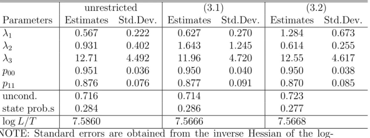
(14) Table 1: Estimates of Structural Parameters of MS Models for (∆gdpt , ∆rt , ∆spt )0 with Lag Order p = 4 and Intercept Term (Sample Period: 1983Q2 − 2006Q3) unrestricted (3.1) (3.2) Parameters Estimates Std.Dev. Estimates Std.Dev. Estimates Std.Dev. λ1 0.567 0.222 0.627 0.270 1.284 0.673 λ2 0.931 0.402 1.643 1.245 0.614 0.255 λ3 12.71 4.492 11.96 4.720 12.55 4.617 p00 0.951 0.036 0.950 0.040 0.950 0.038 p11 0.876 0.076 0.877 0.091 0.870 0.085 uncond. 0.716 0.714 0.723 state prob.s 0.284 0.286 0.277 log L/T 7.5860 7.5666 7.5668 NOTE: Standard errors are obtained from the inverse Hessian of the loglikelihood function. periods. Alternatively, the MS structure may just capture conditional heteroskedasticity which may arise from other sources than the business cycle. Therefore, we have fitted VAR models with MS residuals, assuming that Σ1 6= Σ2 .2 As in Lanne and Lütkepohl (2009) we have estimated an unrestricted model as well as one with the structural restrictions specified in (3.1). In addition, we have also estimated a model with only two zero restrictions on the last column of the matrix of long-run effects,   ∗ ∗ 0 A(1)−1 B =  ∗ ∗ 0  . (3.2) ∗ ∗ ∗ Some estimation results and a range of tests which will be discussed in the following are given in Tables 1-3. The first question of interest is whether the MS model is preferable to the model with mixed normal residuals which was used by Lanne and Lütkepohl (2009). Looking at the estimated state probabilities of the unrestricted model in Table 1 they are both larger than 0.8 and, hence, the states appear to have some persistence. Still, it is desirable to check the MS model against the MN model more formally. Therefore we have performed a likelihood ratio (LR) test of the restriction on the transition matrix specified in (2.5). 2. The computations were done with GAUSS programs using EM iterations to get close to the optimum and then switching to the Newton-Raphson algorithm from the CML library for optimizing the likelihood function.. 9.

(15) Table 2: Wald Tests for Equality of λi ’s for Models from Table 1 unrestricted (3.1) (3.2) H0 test value p-value test value p-value test value p-value λ1 = λ2 = λ3 7.974 0.019 7.739 0.021 7.677 0.022 λ1 = λ2 0.611 0.434 0.630 0.427 0.969 0.325 λ1 = λ3 7.284 0.007 5.645 0.018 6.608 0.010 λ2 = λ3 6.756 0.009 3.869 0.049 5.732 0.017 Table 3: LR Tests of Models for (∆gdpt , ∆rt , ∆spt )0. H0 H1 MN MS (3.1) unrestricted (3.2) unrestricted (3.1) (3.2). Assumed LR statistic distribution 2.959 χ2 (1) 3.491 χ2 (3) 3.456 χ2 (2) 0.036 χ2 (1). p-value 0.085 0.322 0.178 0.850. 1 0.9 0.8. probability of state 0. 0.7 0.6 0.5 0.4 0.3 0.2 0.1 0 1980. 1985. 1990. 1995. 2000. 2005. 2010. Figure 1: Probabilities of State 0 (Pr(st = 0|YT )) for the unrestricted model for (∆gdpt , ∆rt , ∆spt )0 from Table 1.. 10.

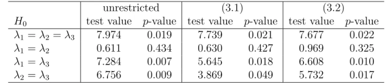
(16) In other words, we test the restriction that the probabilities in each row of P are constant. For this purpose we have reestimated the unrestricted MN model from Lanne and Lütkepohl (2009) and compare the maximum of the likelihood with that of the unrestricted MS model given in Table 1.3 The resulting LR test is reported in Table 3 together with some other LR tests which will be discussed later. The corresponding p-value turns out to be 8.5%. Thus, we can reject the MN model at a 10% level but not at the 5% level. In other words, there is weak evidence in favor of the MS model. Further evidence is provided by the probabilities of being in State 0 which are plotted in Figure 1. More precisely, in Figure 1 we see the state probabilities conditional on the full sample information, Pr(st = 0|YT ), based on the estimated unrestricted model. Obviously, these probabilities are quite persistent. They do not correspond strictly to the phases of the official US business cycle, however. Since one of the λi ’s of the unrestricted model in Table 1 is quite large (λ3 = 12.71) while the other two are around one or a little smaller, the second state is one where at least one of the shocks has a substantially larger volatility than in the first regime. Thus, the state probabilities plotted in Figure 1 correspond to a regime of lower volatility at least in one of the shocks. The corresponding state appears to represent periods when the stock market had a tendency to increase. Notice that the probability of being in this state is low around the stock market crash in 1987 and during the adjustment period after the technology bubble in the first years of the new millennium. In any case, there appears to be some persistence in the state which implies that the MS model may describe the data better than the MN model. Therefore we will now consider the previously used identifying restrictions within our MS model. As mentioned earlier, the zero restrictions in (3.1) and (3.2) are overidentifying if the λi ’s are distinct. Hence, it is instructive to look at the estimates in Table 1. Clearly, the estimated λi ’s of the unrestricted model are quite different. Their standard errors are also quite large, however. Therefore we have performed Wald tests of equality of these quantities and present them in Table 2. These tests have asymptotic χ2 -distributions because the estimators have the usual normal limiting distributions under our assumptions. The p-values reported in Table 2 are based on these χ2 -distributions. In this context it may be worth noting that, in contrast to the matrix B, 3. Since the likelihood is highly nonlinear and has multiple local maxima, it is not uncommon to obtain slightly different results with another estimation algorithm. Therefore it was necessary to reestimate the MN model with our estimation algorithm to ensure strict comparability of the results which is important for a proper comparison of the likelihood maxima. The results in Lanne and Lütkepohl (2009) are qualitatively similar to our estimation results for the MN model although they differ slightly numerically.. 11.

(17) the λi ’s are identified even if they are identical. Thus, testing their equality makes sense. The test that all three λi ’s are equal has a p-value of 1.9% and, hence, clearly rejects at a 5% level. The null hypotheses H0 : λ1 = λ3 and H0 : λ2 = λ3 are even rejected at the 1% level. On the other hand, at common significance levels, it cannot be rejected that λ1 = λ2 . Similar results are also obtained if the restrictions in (3.1) and (3.2) are imposed. Thus, there is strong evidence that at least two of the three λi ’s are distinct. Let us for the moment still pretend that the three λi ’s in the unrestricted model are distinct and, hence, all three shocks are identified without further restrictions on B. In that case, the zero restrictions imposed in (3.1) and (3.2) are overidentifying and can be tested by LR tests. These test results are also given in Table 3. It turns out that none of the zero restrictions can be rejected at conventional significance levels. This result is also obtained when only the additional restriction in the second column of the matrix of long-run effects in (3.1) is tested which was not backed by theoretical considerations (see the last row in Table 3). The resulting p-value is 0.850 and, hence, the data clearly do not object to this restriction. Although this means that we end up with the same model which was used by Binswanger (2004), the advantage of our approach is that the restrictions can be backed by statistical tests. Of course, these conclusions are based on the assumption that all three λi ’s are distinct which does not have strong support from the data. Therefore it is worth reflecting on the implications of some λi ’s being identical. This would mean that some of the restrictions imposed on the matrix of long-run effects in (3.1) and (3.2) may in fact not be overidentifying and, hence, the LR tests may have fewer degrees of freedom than assumed in Table 3. In that case the p-values would be smaller than the ones reported in the table. However, in the absence of further information, we have no basis for rejecting the restrictions in (3.1).. 3.2. European/US Interest Rate Linkages. Our next example is also from Lanne and Lütkepohl (2009). It considers euro area and US interest rate linkages to investigate the relation between European and US monetary policy. It is based on an earlier study by Brüggemann and Lütkepohl (2005) who performed a standard SVAR analysis for cointegrated variables and concluded that European monetary policy depends to some extent on US monetary policy whereas the reverse direction is not apparent from the data. They considered monthly data for a euro area three months money market rate rtEU , a euro area 10-year bond rate RtEU , a US three months money mar12.

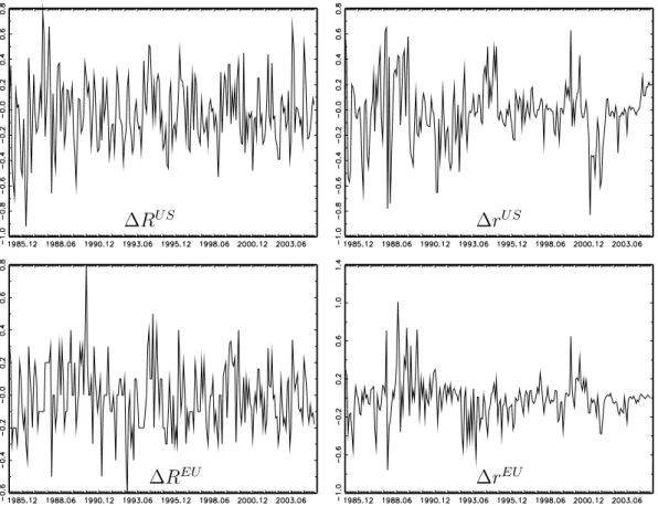
(18) ket rate rtU S and a US 10-year bond rate RtU S . Thus, yt = (RtU S , rtU S , RtEU , rtEU )0 . The sampling period is 1985M 1 − 2004M 12. Details on the data construction and their sources are also given in Appendix B of Lanne and Lütkepohl (2009). Brüggemann and Lütkepohl (2005) found that all four variables are I(1) and that both the expectations hypothesis of the term structure and the uncovered interest rate parity hold. Hence, stationarity of the two spreads RtU S − rtU S and RtEU − rtEU as well as the two parities RtU S − RtEU and rtU S − rtEU is supported. These four relations represent three linearly independent cointegration relations from which the fourth one can be derived by a linear transformation. Therefore Lanne and Lütkepohl (2009) considered a four-dimensional system with three known cointegration relations. They used a VECM for yt with a constant term, three lags of ∆yt (i.e., p = 4), a cointegrating rank of r = 3 and MN residuals to investigate the impact of monetary shocks in the US and in Europe. Again it is easy to think of arguments for a more general MS specification of the residuals and, hence, we have estimated the corresponding MS model and we have tested it against an MN model. Estimation and test results are given in Tables 4-6. They will be discussed in the following. Table 4: Estimates of MS-VECM for (RtU S , rtU S , RtEU , rtEU )0 with Lag Order p = 4, Cointegrating Rank r = 3 and Intercept Term (Sample Period: 1985M 1 − 2004M 12) unrestricted one trans. shock two trans. shocks Parameters Estimates Std.Dev. Estimates Std.Dev. Estimates Std.Dev. λ1 0.812 0.169 0.811 0.168 0.849 0.186 λ2 15.87 3.433 15.90 3.332 14.73 3.232 λ3 3.499 0.807 3.487 0.796 3.386 0.901 λ4 8.422 1.818 8.445 1.802 8.233 1.757 p00 0.904 0.036 0.905 0.036 0.911 0.038 p11 0.919 0.033 0.919 0.033 0.928 0.035 uncond. 0.459 0.458 0.448 state prob.s 0.541 0.542 0.552 log L/T 1.65305 1.65294 1.63751 NOTE: Standard errors are obtained from the inverse Hessian of the loglikelihood function. A test of our unrestricted MS model against an unrestricted MN model, i.e., of the restriction in (2.5) is reported in Table 6. The p-value is extremely small so that the MN model is rejected at any reasonable significance level. Hence, there is strong evidence that the MS model is preferable to the MN 13.

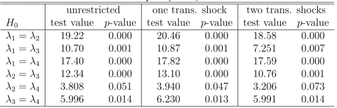
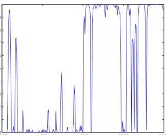
(19) Table 5: Wald Tests for Equality of λi ’s for Models from Table 4 unrestricted one trans. shock two trans. shocks H0 test value p-value test value p-value test value p-value λ1 = λ2 19.22 0.000 20.46 0.000 18.58 0.000 λ1 = λ3 10.70 0.001 10.87 0.001 7.251 0.007 λ1 = λ4 17.40 0.000 17.82 0.000 17.59 0.000 λ2 = λ3 12.34 0.000 13.10 0.000 10.76 0.001 λ2 = λ4 3.808 0.051 3.940 0.047 3.206 0.073 λ3 = λ4 5.996 0.014 6.230 0.013 5.991 0.014 Table 6: LR Tests of Models for (RtU S , rtU S , RtEU , rtEU )0 Assumed H0 H1 LR statistic distribution p-value MN MS 45.39 χ2 (1) 0.000 2 one trans. shock unrestricted 0.051 χ (1) 0.822 2 two trans. shocks unrestricted 7.335 χ (2) 0.026 model for the present data set. This result is not surprising given that the estimated transition probabilities p00 and p11 are both larger than 90% which indicates that the states have considerable persistence. The estimated probabilities of State 0, Pr(st = 0|YT ), are plotted in Figure 2. Three of the λi ’s associated with the unrestricted model in Table 4 are considerably larger than one while the remaining one is not much smaller than one. Hence, overall the volatility in the second state (State 1) is considerably larger than in the first state. The probabilities in Figure 2 are those of the low volatility state. Apparently, the second half of the sample is characterized by lower volatility of shocks to the system. Indeed, the first differences notably of the short-term interest rate series appear to have overall a smaller variability in the second part of the sample except for the period around the year 2000 (see Figure 3). The lower volatility periods correspond to the high probabilities of State 0 in Figure 2. Thus, the states reflect the change in volatility. For our purposes it is important to note that the MS model describes the data better than previous SVAR counterparts. Hence, it is of interest to study its implications for structural analysis. The estimated λi ’s of all the models in Table 4 are quite different. Onestandard error intervals around the estimates do not overlap. Again we have performed Wald tests to check equality of the λi ’s. The results of pairwise tests are presented in Table 5 and confirm distinct λi ’s. The p-values of all pairwise tests are smaller than 10% and most of them are even smaller than 14.

(20) 1 0.9 0.8. probability of state 0. 0.7 0.6 0.5 0.4 0.3 0.2 0.1 0 1985. 1990. 1995. 2000. 2005. Figure 2: Probabilities of State 0 (Pr(st = 0|YT )) for the unrestricted model for (RtU S , rtU S , RtEU , rtEU )0 from Table 4.. 1%. Thus, there is evidence that the λi ’s are distinct and, hence, the shocks can be identified by assuming that they are orthogonal and have identical instantaneous impacts in both states. Consequently, we can check some of the structural assumptions that were used by Brüggemann and Lütkepohl (2005) and Lanne and Lütkepohl (2009). One important conclusion of the previous studies was that there are two transitory shocks which were viewed as candidates for monetary shocks. Since there are three cointegration relations, there can be up to three transitory shocks and Lanne and Lütkepohl (2009) find that the data actually only support two such shocks in their MN framework. This issue is investigated by testing suitable zero restrictions on the matrix of long-term effects of the shocks. is known to be of the form ΞB, where Pp−1This matrix −1 0 0 Ξ = β⊥ [α⊥ (IK − i=1 Γi )β⊥ ] α⊥ and α⊥ and β⊥ signify orthogonal complements of α and β, respectively (e.g., Lütkepohl (2005, Section 9.2)). A shock is transitory if the corresponding column of this matrix consists of zeros. Such restrictions become testable in our MS models because the shocks are identified via the MS structure. LR tests are presented in Table 6. The restrictions associated with one transitory shock (one zero column in ΞB) are not rejected at conventional significance levels whereas two transitory shocks are rejected at the 5% level, the p-value being 0.026. Note that the number of degrees of freedom of the 15.

(21) ∆RU S. ∆rU S. ∆REU. ∆rEU. Figure 3: Changes in interest rates.. 16.

(22) asymptotic χ2 distribution of the LR statistic implied by restricting a column of ΞB to zero take into account the reduced rank of the matrix of long-run effects. In particular, since the cointegrating rank is three, the (4 × 4) matrix ΞB has rank one so that a zero column of ΞB stands for a single restriction. Thus, in our model, the data do not support the existence of two transitory shocks. Assuming one transitory shock only, we have also tested a number of alternative restrictions on its effects which did not help in determining a specific interpretation of this shock. In particular, we cannot identify it as a US or European monetary policy shock. Thus, we find little support for assumptions that allow us to explore the relation between US and European monetary shocks. Consequently, we do not find evidence for the hypothesis that US monetary policy has a more important impact on European monetary policy than vice versa. Thus, using the MS framework sheds doubt on whether the matter can be settled within a simple model of this type.. 4. Conclusions. In this study we have augmented VAR models by Markov switching to obtain identified shocks. We have shown that under general conditions it is enough to assume orthogonality of the shocks and invariance of the impulse responses across regimes to obtain identification. A main advantage of this setup is that the data are informative with respect to the additional conditions needed for identification. Moreover, other assumptions which are typically used in SVAR analysis become overidentifying in our framework and, hence, are testable. We have applied these ideas to two SVAR models from the literature where a MS structure in the residual volatility is plausible. In the first example a US macro system consisting of GDP, an interest rate and a stock price index is analyzed and it is found that in our framework previously assumed identifying restrictions can be confirmed. In the second example the interest rate linkage between the US and the euro area is investigated. The MS model is found to be a better description of the data than previous SVAR models. Thus, it makes sense to use our framework for testing previously made identifying assumptions against the data. It turns out that a crucial restriction cannot be confirmed in our framework. Overall our setup appears to be a useful tool to extract more information on identifying assumptions in SVAR analysis from the data. The limited knowledge on the statistical inference procedures in particular when cointegrated variables are considered offer directions for further 17.

(23) research. Moreover, the numerical challenges in estimating the models are nonnegligible if larger models with many variables and states are of interest. The algorithms proposed by Sims et al. (2008) may be useful in this context and may help to overcome numerical problems in difficult situations. Further investigations in this direction are also left for the future.. Appendix. A Uniqueness Result for Covariance Matrix Decomposition Proposition A. Let Σ0 = BB 0 and Σi = BΛi B 0 , where Λi = diag(λi1 , . . . , λiK ), i = 1, . . . , M , be nonsingular (K ×K) covariance matrices. Then the (K ×K) matrix B in the decomposition Σ0 = BB 0 is unique apart from sign reversal of its columns if for all k 6= j ∈ {1, . . . , K} there exists an i ∈ {1, . . . , M } such that λik 6= λij . ¤ Proof: Suppose Q = [qij ] is a (K × K) matrix such that Σ0 = BB 0 = BQQ0 B 0. (A.1). and Σi = BΛi B 0 = BQΛi Q0 B 0 ,. i = 1, . . . , M.. (A.2). To show the uniqueness of B up to multiplication of its columns by −1, we have to show that the only feasible matrix Q is a diagonal matrix with ±1 on the main diagonal. Pre- and post-multiplying (A.1) by B −1 and its transpose, respectively, implies that QQ0 = IK and, hence, Q must be orthogonal. Similarly, it follows from (A.2) that QΛi Q0 = λi or QΛi = Λi Q, i = 1, . . . , M . Consequently, λik qkl = λil qkl for all i = 1, . . . , M . Thus, qkl = 0 for k 6= l because λik 6= λil for at least one i ∈ {1, . . . , M }. In other words, Q is an orthogonal diagonal matrix and, hence, all diagonal elements of Q are ±1 because the diagonal elements of a diagonal matrix are its eigenvalues and the eigenvalues of a diagonal real orthogonal matrix are all ±1. This proves the proposition.. References Amisano, G. and Giannini, C. (1997). Topics in Structural VAR Econometrics, 2nd edn, Springer, Berlin. Binswanger, M. (2004). How do stock prices respond to fundamental shocks?, Finance Research Letters 1: 90–99.. 18.

(24) Blanchard, O. and Quah, D. (1989). The dynamic effects of aggregate demand and supply disturbances, American Economic Review 79: 655–673. Brüggemann, R. and Lütkepohl, H. (2005). Uncovered interest rate parity and the expectations hypothesis of the term structure: Empirical results for the U.S. and Europe, Applied Economics Quarterly 51: 143–154. Canova, F. and De Nicoló, G. (2002). Monetary disturbances matter for business fluctuations in the G-7, Journal of Monetary Economics 49: 1131–1159. Christiano, L. J., Eichenbaum, M. and Evans, C. (1999). Monetary policy shocks: What have we learned and to what end?, in J. B. Taylor and M. Woodford (eds), Handbook of Macroeconomics, Vol. 1A, Elsevier, Amsterdam, pp. 65– 148. Douc, R., Moulines, E. and Rydén, T. (2004). Asymptotic properties of the maximum likelihood estimator in autoregressive models with Markov regime, Annals of Statistics 32: 2254–2304. Faust, J. (1998). The robustness of identified VAR conclusions about money, Carnegie-Rochester Conference Series in Public Policy 49: 207–244. Francq, C. and Roussignol, M. (1997). On white noise driven by hidden Markov chains, Journal of Time Series Analysis 18: 553–578. Hamilton, J. D. (1989). A new approach to the economic analysis of nonstationary time series and the business cycle, Econometrica 57: 357–384. Hamilton, J. D. (1994). Time Series Analysis, Princeton University Press, Princeton, New Jersey. Johansen, S. (1995). Likelihood-based Inference in Cointegrated Vector Autoregressive Models, Oxford University Press, Oxford. King, R. G., Plosser, C. I., Stock, J. H. and Watson, M. W. (1991). Stochastic trends and economic fluctuations, American Economic Review 81: 819–840. Koop, G. (1992). Aggregate shocks and macroeconomic fluctuations: A Bayesian approach, Journal of Applied Econometrics 7: 395–411. Krolzig, H.-M. (1997). Markov-Switching Vector Autoregressions: Modelling, Statistical Inference, and Application to Business Cycle Analysis, SpringerVerlag, Berlin. Lanne, M. and Lütkepohl, H. (2008). Identifying monetary policy shocks via changes in volatility, Journal of Money, Credit and Banking 40: 1131–1149. Lanne, M. and Lütkepohl, H. (2009). Structural vector autoregressions with nonnormal residuals, Journal of Business & Economic Statistics, forthcoming.. 19.

(25) Lütkepohl, H. (1996). Handbook of Matrices, John Wiley & Sons, Chichester. Lütkepohl, H. (2005). New Introduction to Multiple Time Series Analysis, Springer-Verlag, Berlin. Pagan, A. R. and Pesaran, M. H. (2008). Econometric analysis of structural systems with permanent and transitory shocks, Journal of Economic Dynamics and Control 32: 3376–3395. Rapach, D. E. (2001). Macro shocks and real stock prices, Journal of Economics and Business 53: 5–26. Rigobon, R. (2003). Identification through heteroskedasticity, Review of Economics and Statistics 85: 777–792. Rubio-Ramirez, J. F., Waggoner, D. and Zha, T. (2005). Markov-switching structural vector autoregressions: Theory and applications, Discussion Paper, Federal Reserve Band of Atlanta. Sims, C. A. (1980). Macroeconomics and reality, Econometrica 48: 1–48. Sims, C. A., Waggoner, D. F. and Zha, T. (2008). Methods for inference in large multiple-equation Markov-switching models, Journal of Econometrics 146: 255–274. Sims, C. A. and Zha, T. (2006). Were there regime switches in U.S. monetary policy?, American Economic Review 96: 54–81. Uhlig, H. (2005). What are the effects of monetary policy on output? Results from an agnostic identification procedure, Journal of Monetary Economics 52: 381–419.. 20.

(26)

No results found