LOCALIZATION-FREE POWER CARTOGRAPHY
Yves Teganya, Luis M. Lopez-Ramos, Daniel Romero, and Baltasar Beferull-Lozano
WISENET Lab., Dept. of ICT, University of Agder, Grimstad, Norway
ABSTRACT
Spectrum cartography constructs maps of metrics such as channel gain or received signal power across a geographic area of interest using measurements of spatially distributed sensors. Applications of these maps include network plan-ning, interference coordination, power control, localization, and cognitive radio to name a few. Existing spectrum car-tography methods necessitate knowledge of sensor locations, but such locations cannot be accurately determined from pilot positioning signals (such as those in LTE or GPS) in indoor or dense urban scenarios due to multipath. To circumvent this limitation, this paper proposes localization-free cartography, where spectral maps are directly constructed from features of these positioning signals rather than from location esti-mates. The proposed algorithm capitalizes on the framework of kernel-based learning and offers improved prediction per-formance relative to existing alternatives, as demonstrated by a simulation study in a street canyon.
Index Terms— Spectrum cartography, localization-free cartography, kernel-based learning, spectrum map.
1. INTRODUCTION
Spectrum cartography constructs maps of a certain channel metric, such as received signal power, interference power, or channel gain over the geographical area of interest [1–3]. Spectral maps are of utmost interest in wireless networks, es-pecially for tasks such as network planning, interference coor-dination, power control, and dynamic spectrum access [4–6]. Further applications include source localization [2].
Existing approaches typically apply some spatial interpo-lation or regression technique to measurements collected by spatially distributed sensors. Examples of these approaches for mapping power over space include kriging [1, 7, 8], com-pressive sensing [3], matrix completion [9], dictionary learn-ing [10, 11], Bayesian models [12], and adaptive radial basis functions [13]. Schemes to map power spectral density (PSD) have also been devised by exploiting the sparsity of power dis-tribution over space and frequency [2] and by leveraging the
Dept. of ICT, University of Agder, Jon Lilletunsvei 3, Grim-stad, 4879 Norway. Emails:{yves.teganya,luismiguel.lopez,daniel.romero, baltasar.beferull}@uia.no. This work was supported by the FRIPRO TOPP-FORSK grant 250910/F20 and the INFRASTRUCTURE ReRaNP grant 245699/F50 from the Research Council of Norway.
frameworks of thin-plate spline regression [4, 14] and kernel-based learning [4]. Further schemes have been proposed to map alternative metrics such as channel gain [15–17].
Since all the aforementioned schemes rely on the knowl-edge of the sensor locations, they will be collectively referred to aslocalization-based cartography. In practice, location is seldom known and therefore it must be estimated from fea-tures such as the RSSI, the time (difference) of arrival, or the direction of arrival of positioning pilot signals transmitted by satellites (e.g. in GPS) or terrestrial base stations (e.g. in LTE or WiFi [18]). Unfortunately, accurate location estimates are often not available in practice due to propagation phenom-ena affecting those pilot signals such as multipath, which lim-its the applicability of existing cartography techniques, espe-cially in indoor and dense urban scenarios.
The main contribution of this paper is to circumvent this limitation by proposing localization-free cartography. The idea is that the localization step introduces significant errors in the spectrum map estimation when the aforementioned features are not reliable. Bypassing this step, the proposed approach obtains spectrum maps indexed directly by (or as a function of) the features of the received pilots. As a byproduct of skipping the localization step, the resulting car-tography algorithm is also computationally less expensive than its localization-based counterparts. For simplicity, this work focuses on constructing power maps, but the proposed algorithm carries over to other metrics. Such an algorithm is developed within the framework of kernel-based learning not only because of the high simplicity, flexibility, and per-formance of kernel-based estimators, but also because it has well-documented merits in spectrum cartography [4, 14].
The rest of this paper is organized as follows: Sec. 2 de-scribes the problem and reviews location-based cartography. Sec. 3 presents the main contribution of the paper, which is localization-free cartography. Simulations and conclusions are respectively provided in Sec. 4 and Sec. 5.
2. PRELIMINARIES
The goal is to determine the powerp(x)of a certain channel, termedchannel-to-map (C2M), at every locationx ∈ X of the geographical region X ⊂ R2 of interest. To this end, N sensors are deployed across X at locations{xn}N
n=1not
˜
pnof the powerp(xn)at its locationxn.
In localization-based cartography, a fusion center is ide-ally given pairs{(xn,p˜n)}Nn=1, which include the exact
sen-sor locations{xn}Nn=1, and obtains a function estimatepˆ(xq)
that provides the power of the C2M at any query location
xq ∈ X. With this function, a node at xq can determine
the power of the C2M if it knowsxq. In practice, however,
location is typically unknown and hence then-th sensor must estimatexnby relying on pilot signals{ym,n[k]}Mm=1, where ym,n[k]denotes thek-th sample of them-th pilot signal re-ceived by then-th sensor. For convenience, form theM×K
matrixYn whose (m, k)-th entry isym,n[k]. From Yn, the
n-th sensor computes an estimatexˆn(Yn)of xn by means
of some localization algorithm; see Sec. 4 for a specific ex-ample. The fusion center then uses{(ˆxn,p˜n)}Nn=1to obtain
an estimatepˆ(x)of the function p(x). Therefore, if the lo-cation estimates{xˆn}Nn=1 are noisy, so will be pˆ(x). If a
node at a query locationxqwishes to know the power of the
C2M, it will use the pilot signals Yq to obtain an estimate ˆ
xq := ˆx(Yq)of its location and will evaluate the map
esti-mate aspˆ(ˆxq). Here,Yq is a matrix whose(m, k)-th entry
is given by thek-th sample of them-th pilot signalym,q[k]
at the query locationxq. Thus, such an evaluation has two
sources of error: first, the location estimation error inxˆqand,
second, the map estimation error inpˆ(xq).
From a more general perspective, the function that is ac-tually learned in this approach can be expressed asp(Y) :=
p(ˆx(Y)), where xˆ(Y)denotes the output of the chosen lo-calization algorithm when the pilot signals are given byY. From this perspective, the problem that is being solved is: given{(Yn,p˜n)}Nn=1, find an estimatepˆ(Y)ofp(Y). Indeed,
localization-based cartography seeks an estimate for the latter function within a certain family of functions that can be ex-pressed asp(Y) =g(ˆx(Y))for some functiong :X →R.
The next section investigates estimates with alternative forms, which will be preferable wheneverxˆ(Y)is not an accurate estimator ofx.
Remark 1 One may argue that a node can determine the power of the C2M at its location more efficiently by measuring it rather than by locating itself and evaluating a map. While this may be the case for a single C2M, determining the power of many C2Ms, or other channel parameters such as the im-pulse response, may incur a higher cost. In these cases, the benefits of spectrum cartography would be more significant.
3. LOCALIZATION-FREE CARTOGRAPHY
This section proposes localization-free cartography, which bypasses the localization step involved in all existing raphy approaches. To this end, the localization-free cartog-raphy problem is formulated as a function estimation task in Sec. 3.1 and solved via kernel-based learning in Sec. 3.2.
3.1. Map Estimate as a Function Composition
From an abstract perspective, spectrum cartography amounts to learning a function p : CM×K →
R that provides the
powerp(Y)of the C2M at a location inX where the pilot signalsY are received. Thedirect approachto spectrum car-tography would be to learn such a function directly from data
{(Yn,p˜n)}Nn=1. Since learning a multivariate function up to
a reasonable accuracy generally requires the number of data points to be several times larger than the number of input vari-ables, the direct approach would needN to be significantly larger thanM K, which is prohibitively large sinceM K is typically in the order of hundreds or thousands. For this rea-son, existing (localization-based) cartography schemes do not follow such a direct approach. Instead, they avoid its com-plexity by confining the search for estimates ofp(Y)to those functions that can be expressed as the composition of a fixed functionxˆ : CM×K → X ⊂
R2, wherexˆ(Y)corresponds
to the output of a localization algorithm when the pilot sig-nals areY, and a map functiong :X ⊂R2→Rthat needs
to be determined; (cf. Sec. 2). Clearly, findingg requires a significantly smallerN than learning the general function
p: CM×K → Rsinceg has only two scalar inputs. When
ˆ
x(Y)is a reasonable estimate of the locationxat whichY
has been observed, such a localization-based approach works well. However, due to propagation effects impacting the pi-lot signals inY,xˆ(Y)may be very different fromxand it is easy to see that this drastically hinders the estimation of
g. From this observation, it can be concluded that the two scalar outputs ofxˆ(Y)fail to capture the relevant informa-tion inY: more outputs are needed. In summary, neither the above direct approach, which estimates a function withM K
inputs, nor the localization-based approach, which estimates a function of 2 inputs, are appropriate in presence of multipath effects, as is the case in indoors or urban scenarios.
To tackle this difficulty, the proposed approach is to es-timate a function whose number of inputs is larger than 2 and smaller thanM K. To answer the question on which in-puts should be used, it is worth delving further into why the above localization-based approach fails. Localization algo-rithms typically proceed in two steps: first, they extract some featuresfromY, and then they feed these features to an algo-rithmLthat exploits a spatial model to determine the location. Those features comprise e.g. estimates of distance, time (dif-ference) of arrival, or angle of arrival. Ifφ(Y) ∈ D ⊂RM
denotes the vector stacking theseMfeatures andl(φ)denotes the output of algorithmL, it follows thatxˆ(Y) =l(φ(Y)). The root of the problem is therefore that the model assumed byLis inaccurate: it typically assumes free space propaga-tion, which would imply a certain consistency between the features inφ(Y)that does not hold in presence of multipath. Combining these observations, a sensible approach is to (i) preserve the dimensionality reduction capability ofφ(from
one can seeklocalization-freefunction estimates of the form
ˆ
pLF(Y) = f(φ(Y))for somef : D ⊂ RM → R. In this
localization-free setup, φ(Y) comprises M features of the pilot signals, but they need not be those used by the localiza-tion algorithms (e.g. time (difference) or angle of arrival). In short, whereas localization-based cartography learns a func-tion of the spatial locafunc-tion estimated from features of the pi-lot signals, the proposed localization-free approach directly learns a function of such features.
3.2. Kernel-based Power Map Learning
This section provides a kernel-based learning algorithm to learn the function f introduced in Sec. 3.1. Given pairs
{(φn,p˜n)} N
n=1, whereφn:=φ(Yn), the regression problem
is informally to findf such thatf(φ(Y))≈p(Y)for allY. To address this problem, one must specify in which family of functions such anfmust be found. In kernel-based learning, one seeksf in a set known as areproducing-kernel Hilbert space(RKHS) and given by
F:= ( f :f(φ) = ∞ X i=1 αiκ(φ,φ¯i), φ¯i∈ D, αi ∈R ) ,
whereκ : D × D → R is a symmetric and positive def-inite function known as reproducing kernel [19]. A com-mon choice is the so-called Gaussian radial basis function
κ(φ,φ0) := exp
−kφ−φ0k2/(2σ2)
, whereσis a param-eter selected by the user. Like any Hilbert space,F has an associated inner product and norm. For an RKHS function
f(φ) =P∞
i=1αiκ(φ,φ¯i), the latter is given by kfk2F := ∞ X i=1 ∞ X j=1 αiαjκ( ¯φi,φ¯j). (1)
Kernel-based learning typically solves a problem of the form
ˆ f = arg min f∈F 1 N N X n=1 L(˜pn,φn, f(φn)) + Ω(kfkF), (2)
where Lis a loss function quantifying the deviation between the observations {˜pn}N
n=1 and the predictions {f(φn)}Nn=1
returned by a candidatef; andΩis an increasing function. The first term in (2) promotes function estimates that fit well the data whereas the second term promotes “smooth” esti-mates; where the notion of smoothness is determined by the RKHS normk · kF. Typical choices areL(˜pn,φn, f(φn)) = (˜pn −f(φn))2 and Ω(kfkF) = λkfk
2
F, where λ > 0 is termed regularization parameter and balances smoothness and goodness of fit. For this choice,fˆis termedkernel ridge re-gressionestimate [20], and is the one pursued here for sim-plicity. The goal is therefore to solve (2). However, since
F is infinite dimensional in general, (2) cannot be directly solved. Fortunately, one can invoke the representer theo-rem[19], which states that the solution to (2) is of the form
ˆ f(φ) = N X n=1 αnκ(φ,φn). (3) for some{αn}N
n=1. Although the representer theorem does
not provide the coefficients{αn} N
n=1, they can be obtained
by substituting (3) into (2) and solving the resulting problem with respect to these coefficients. Applying this procedure for kernel ridge regression results in the problem
ˆ α= arg min α 1 N k˜p−Kαk 2 +λα>Kα, (4) where α:= [α1, ..., αN]>,p˜ := [˜p1, ...,p˜N]>, andKis an
N×N matrix whose(n, n0)-th entry isκ(φn,φn0). Prob-lem (4) can be solved in closed form as
ˆ
α= (K+λNIN)−1p˜. (5)
The estimatefˆsolving (2) for kernel ridge regression can be recovered by substituting (5) into (3). To obtain the predicted power of the C2M at a query locationxqwhere the pilot
sig-nals are given byYq, one just evaluatespˆLF(Yq) = ˆf(φ(Yq)).
4. NUMERICAL TESTS
This section evaluates the performance of localization-free cartography in a scenario with multipath. The latter is aurban canyonorstreet canyon, which comprises two parallel verti-cal planes modeling the walls (or buildings) at each side of the street and a horizontal plane modeling the ground. Prop-agation is characterized by the so calledsix-ray model[21], which accounts for the direct path, the ground reflection, 2 first-order wall reflections, and 2 wall-to-wall second-order reflections. The sensors are spread uniformly at random over the street, which is250m long and30m wide.
For simplicity, the pilot signals are impulses centered at time 0 filtered to the pilot channel with bandwidth 5 MHz and carrier frequency 800 MHz, which implies thatYncomprises
the impulse responses of the bandlimited channels between theM transmitters of pilot signals and then-th sensor. For simplicity and robustness to timing errors, the features used by the proposed localization-free algorithm equal the cen-ter of mass of the corresponding impulse responses, that is,
[φn]m := PK k=1tk|ym,n[k]| 2/PK k=1|ym,n[k]| 2wheret k is
the time of thek-th sample.
The proposed algorithm, which uses Gaussian radial basis functions withσ = 30m, is compared with its localization-based counterpart, which is a special case of the estimators in [2, 4, 22] for estimating power maps. We use Gaussian RBFs because they are universal kernels [23], i.e., able to approximate arbitrary functions. For localization, the square-range-based least squares (SR-LS) algorithm [24] is applied to the time-of-arrival measurements obtained from the pilots {Yn}N
n=1. Function g (cf. Sec. 2) is
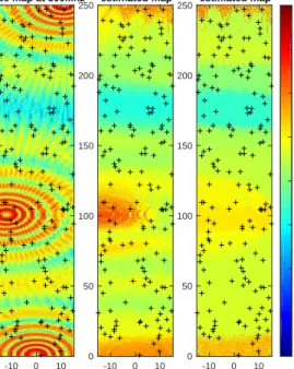
True map at 800Mhz -10 0 10 x[m] 0 50 100 150 200 250 y[m] Localization-free estimated map -10 0 10 x[m] 0 50 100 150 200 250 Localization-based estimated map -10 0 10 x[m] 0 50 100 150 200 250 -50 -45 -40 -35 -30 -25 -20 -15 -10 dBW
Fig. 1: (a) True map, (b) localization-free, and (c) localization-based estimated maps (λ= 3×10⁻³,N= 160).
localization-free algorithm: Given {(ˆxn,p˜n)} N
n=1, the
esti-mate ofgis given byg(ˆxq) =κ0>(ˆxq) ˆβwhere κ0(ˆxq) := [κ0(ˆxq,x1ˆ ), ..., κ0(ˆxq,xˆN)]>, βˆ = (K0+λNIN)−1p˜, and
K0is anN×N matrix with(n, n0)-th entryκ0(ˆxn,xˆn0)and
κis a Gaussian radial basis function withσ= 35m.
Quantitative evaluation will compare the normalized mean square error (NMSE) defined as NMSE=E{|p(x)−
ˆ
p(Y(x) +Υ,T)|2}/
E{|p(x)−p¯|2}whereY(x)comprises
the received pilot signals at locationx,Υrepresents noise,
¯
pis the spatial average of p(x), and T is the training set, defined asT := {(Yn +Υn,p˜n +n)}Nn=1 with Υn and
nrepresenting noise. Specifically,{n}Nn=1are independent
log-normal random variables with zero-mean and standard deviation 0.5 dB (p˜nis measured in dBW). FurthermoreE{·}
denotes expectation over a random location x uniformly distributed acrossX, the locations of the sensors, and noise.
The true map generated through the canyon model is de-picted to the left of Fig. 1. The middle and right panels re-spectively show the localization-free and localization-based map estimates, which are obtained by placing a query sen-sor at each location. Black crosses indicate the positions of the N sensors used to estimate the map. As expected, the estimation is better in areas with more sensors. Visually, the quality of the localization-free estimate is higher than that of the localization-based estimate due to multipath.
Fig. 2a shows the NMSE as a function ofN for differ-ent numbersM of pilot signals. Each point is obtained by
20 40 60 80 100 120 140 160 Number of sensors, N 0.6 0.8 1 1.2 1.4 NMSE M=1 M=2 M=3 20 40 60 80 100 120 140 160 Number of sensors, N 0.6 0.8 1 1.2 NMSE LocFree LocBased
Fig. 2: (a) Estimated map NMSE for different values of num-ber of features, M and sensors, N; and (b) Performance comparison between the localization-free cartography and the localization-based cartography (λ= 3×10⁻³,σ= 30m).
averaging 200 independent Monte Carlo iterations. As antici-pated, performance improves withN. Furthermore, for fixed
N, the NMSE is non-increasing withM, yetM = 2and3
yield roughly the same NMSE because of the geometry of the simulation setup.
Fig. 2b shows the NMSE as a function of the number of sensors N used to estimate pLF and pLB. With significant evidence, one may claim that the proposed localization-free cartography scheme outperforms its localization-based coun-terpart when N > 60 since the error bars in Fig. 2 span over 6 standard deviations of the NMSE across realizations. The reason for a poorer performance of the localization-based scheme is that multipath propagation can mislead the local-ization algorithm, inducing errors in location estimation that increase deviations in the map estimation as well.
5. CONCLUSIONS
Localization-free cartography has been proposed as an alter-native to classic localization-based schemes, which do not operate properly when multipath impairs the propagation of localization pilot signals. Kernel-ridge regression was ap-plied to estimate power maps from features of those pilot signals collected by a number of sensors. Simulations cor-roborate the merits of localization-free cartography relative to localization-based methods. Future research will include an extensive simulation study in indoor environments and de-velop distributed and online extensions.
6. REFERENCES
[1] A. Alaya-Feki, S. B. Jemaa, B. Sayrac, P. Houze, and E. Moulines, “Informed spectrum usage in cognitive ra-dio networks: Interference cartography,” inProc. IEEE Int. Symp. Personal, Indoor Mobile Radio Commun., 2008, pp. 1–5.
[2] J.-A. Bazerque and G. B. Giannakis, “Distributed spec-trum sensing for cognitive radio networks by exploiting sparsity,” IEEE Trans. Sig. Process., vol. 58, no. 3, pp. 1847–1862, Mar. 2010.
[3] B. A. Jayawickrama, E. Dutkiewicz, I. Oppermann, G. Fang, and J. Ding, “Improved performance of spec-trum cartography based on compressive sensing in cog-nitive radio networks,” inProc. Int. Conf. Commun.,, 2013, pp. 5657–5661.
[4] D. Romero, S.-J. Kim, G. B. Giannakis, and R. Lopez-Valcarce, “Learning power spectrum maps from quan-tized power measurements,” IEEE Trans. Sig. Process., vol. 65, no. 10, pp. 2547–2560, 2017.
[5] S. Grimoud, S. B. Jemaa, B. Sayrac, and E. Moulines, “A rem enabled soft frequency reuse scheme,” inProc. IEEE Global Commun. Conf., 2010, pp. 819–823. [6] E. Dall’Anese, S.-J. Kim, G. B. Giannakis, and
S. Pupolin, “Power control for cognitive radio networks under channel uncertainty,”IEEE Trans. Wireless Com-mun., vol. 10, no. 10, pp. 3541–3551, 2011.
[7] G. Boccolini, G. Hernandez-Penaloza, and B. Beferull-Lozano, “Wireless sensor network for spectrum cartog-raphy based on kriging interpolation,” inProc. IEEE Int. Symp. Personal, Indoor Mobile Radio Commun., 2012, pp. 1565–1570.
[8] W.C.M.V. Beers and J.P.C. Kleijnen, “Kriging interpo-lation in simuinterpo-lation: a survey,” inProc. IEEE Winter Simulation Conf., 2004, vol. 1, pp. 113–121.
[9] G. Ding, J. Wang, Q. Wu, Y.-D. Yao, F. Song, and T. A Tsiftsis, “Cellular-base-station-assisted device-to-device communications in tv white space,”IEEE J. Sel. Areas Commun., vol. 34, no. 1, pp. 107–121, 2016. [10] S.-J. Kim, N. Jain, G. B Giannakis, and P. A. Forero,
“Joint link learning and cognitive radio sensing,” in Proc. Asilomar Conf. Sig., Syst., Comput., 2011, pp. 1415–1419.
[11] S.-J. Kim and G. B. Giannakis, “Cognitive radio spec-trum prediction using dictionary learning,” in Proc. IEEE Global Commun. Conf., 2013, pp. 3206–3211. [12] D.-H. Huang, S.-H. Wu, W.-R. Wu, and P.-H. Wang,
“Cooperative radio source positioning and power map
reconstruction: A sparse bayesian learning approach,” IEEE Trans. Veh. Technol., vol. 64, no. 6, pp. 2318– 2332, 2015.
[13] M. Hamid and B. Beferull-Lozano, “Non-parametric spectrum cartography using adaptive radial basis func-tions,” in Proc. IEEE Int. Conf. Acoust., Speech, Sig. Process., 2017, pp. 3599–3603.
[14] J.-A. Bazerque, G. Mateos, and G. B. Giannakis, “Group-lasso on splines for spectrum cartography,” IEEE Trans. Sig. Process., vol. 59, no. 10, pp. 4648– 4663, Oct. 2011.
[15] S.-J. Kim, E. Dall’Anese, and G. B. Giannakis, “Co-operative spectrum sensing for cognitive radios using kriged kalman filtering,” IEEE J. Sel. Topics Sig. Pro-cess., vol. 5, no. 1, pp. 24–36, 2011.
[16] D. Romero, D. Lee, and G. B. Giannakis, “Blind chan-nel gain cartography,” inProc. IEEE Global Conf. Sig. Inf. Process., 2016, pp. 1110–1115.
[17] D. Lee, S.-J. Kim, and G. B. Giannakis, “Channel gain cartography for cognitive radios leveraging low rank and sparsity,” IEEE Trans. Wireless Commun., vol. 16, no. 9, pp. 5953–5966, 2017.
[18] M. Bshara, U. Orguner, F. Gustafsson, and L. Van Biesen, “Fingerprinting localization in wireless networks based on received-signal-strength measurements: A case study on wimax networks,” IEEE Trans. Veh. Technol., vol. 59, no. 1, pp. 283–294, 2010.
[19] B. Sch¨olkopf, R. Herbrich, and A. J. Smola, “A gen-eralized representer theorem,” inProc. Computational Learning Theory. Springer, 2001, pp. 416–426.
[20] C. M. Bishop,Pattern Recognition and Machine Learn-ing, Information Science and Statistics. Springer, 2006. [21] F. P´erez Font´an and P. Mari˜no Espi˜neira, Modeling the wireless propagation channel: a simulation approach with Matlab, Wiley, 2008.
[22] J.-A. Bazerque and G. B. Giannakis, “Nonparametric basis pursuit via kernel-based learning,”IEEE Sig. Pro-cess. Mag., vol. 28, no. 30, pp. 112–125, Jul. 2013. [23] C. A. Micchelli, Y. Xu, and H. Zhang, “Universal
ker-nels,” Journal of Machine Learning Research, vol. 7, no. Dec, pp. 2651–2667, 2006.
[24] A. Beck, P. Stoica, and J. Li, “Exact and approximate solutions of source localization problems,”IEEE Trans. Sig. Process., vol. 56, no. 5, pp. 1770–1778, 2008.