Statistical Methods in Metabolomics

(1)

University of London

Imperial College of Science, Technology and Medicine

Department of Epidemiology & Biostatistics

Statistical Methods in Metabolomics

Harriet Jane Muncey

Supervised by Dr Maria De Iorio & Dr Tim Ebbels

Submitted in part fulfilment of the requirements for the degree of

Doctor of Philosophy in Epidemiology & Biostatistics of the University of London and the Diploma of Imperial College, October 16, 2014

(2)

(3)

Declaration

The copyright of this thesis rests with the author and is made available under a Creative Commons Attribution Non-Commercial No Derivatives licence. Researchers are free to copy, distribute or transmit the thesis on the condition that they attribute it, that they do not use it for commercial purposes and that they do not alter, transform or build upon it. For any reuse or redistribution, researchers must make clear to others the licence terms of this work.

I herewith certify that all material in this dissertation which is not my own work has been properly acknowledged.

Harriet Muncey

(4)

(5)

Abstract

Metabolomics lies at the fulcrum of the system biology ‘omics’. Metabolic profiling offers researchers new insight into genetic and environmental interactions, responses to pathophysi-ological stimuli and novel biomarker discovery. Metabolomics lacks the simplicity of a single data capturing technique; instead, increasingly sophisticated multivariate statistical techniques are required to tease out useful metabolic features from various complex datasets. In this work, two major metabolomics methods are examined: Nuclear Magnetic Resonance (NMR) Spec-troscopy and Liquid Chromatography-Mass Spectrometry (LC-MS). MetAssimulo, an1_H-NMR metabolic-profile simulator, was developed in part by this author and is described in the Chap-ter 2. Peak positional variation is a phenomenon occurring in NMR spectra that complicates metabolomic analysis so Chapter 3 focuses on modelling the effect of pH on peak position. Analysis of LC-MS data is somewhat more complex given its 2-D structure, so I review existing pre-processing and feature detection techniques in Chapter 4 and then attempt to tackle the issue from a Bayesian viewpoint. A Bayesian Partition Model is developed to distinguish chro-matographic peaks representing useful features from chemical and instrumental interference and noise. Another of the LC-MS pre-processing problems, data binning, is also explored as part of H-MS: a pre-processing algorithm incorporating wavelet smoothing and novel Gaussian and Exponentially Modified Gaussian peak detection. The performance of H-MS is compared alongside two existing pre-processing packages: apLC-MS and XCMS.

(6)

(7)

Dedication

For Silvia; who showed me my strength.

(8)

(9)

Acknowledgements

I would like to thank Dr Maria De Iorio and Dr Timothy Ebbels for their invaluable expert guidance and patience during my PhD research. I would like to acknowledge Paul Benton, Imperial College London, for his expert advice in getting to grips with XCMS and Will Astle for his patient help in understanding NMR data.

I also thank Laura Egnash and Michael Reilly, formerly of the Department of Discovery Biomarkers, Pfizer Global R&D, Ann Arbor, MI, for providing the Synthetic Urine data used in testing the H-MS algorithm in Chapter 4. Alexander Amberg of Sanofi-Aventis Deutsch-land GmbH, DSAR Preclinical Safety, Frankfurt, Germany, is acknowledged for providing the Standard Dilution Series data also used in the testing of H-MS. Dr Elizabeth Want of Imperial College London enabled me access to the LC-MS datasets used in Chapter 4. Gregory Tredwell, Imperial College London, kindly provided the 1_{H-NMR data used in Chapter 3. My financial} support is acknowledged from an MRC Capacity Building PhD Studentship.

I am unbelievably grateful to my friends, in particular Lizzy, Laurie and Ratchet for their unfaltering support throughout my academic career. From extreme study sessions during my undergraduate degree to random nonsense and escapades in Durham, London and many other places; they have always been there to both support and distract me as well as keep me going. Highlights include The Sandwich of Dreams, Pie, Quiche and of course Flan. I would also like to thank my family for their love and understanding, and without whom I never would have got this far. Lastly, but by no means least, I wish to thank Silvia for showing me back to my path and helping me realise it was worth it.

(10)

(11)

List of Tables

3.1 Number of protonation sites for each metabolite studied. Where multiple reso-nances are used for a single metabolite these are labeled numerically. . . 47 3.2 Actual pKa values vs Posterior Mean pKa Estimates and Variance from MCMC

simulation using rjags package and MATLAB function nlinfit pKa Estimates with mean squared error (MSE) values. . . 57 3.3 Akaike Information Criterion values for 1, 2 and 3 Site Models fitted to all the

metabolites, alongside actual number of sites of each molecule. Smallest values are shown in bold, indicating chosen model. . . 57 3.4 Bayesian Information Criterion values for 1, 2 and 3 Site Models fitted to all the

metabolites, alongside actual number of sites of each molecule. Smallest values are shown in bold, indicating chosen model. . . 58 3.5 Deviance Information Criterion values for 1, 2 and 3 Site Models fitted to all the

metabolites, alongside actual number of sites of each molecule. Smallest values are shown in bold, indicating chosen model. . . 58 3.6 Actual number of free parameters for appropriate model andpD values (estimated

number of effective parameters) for each model. . . 59 3.7 Log Pseudo Marginal Likelihood values for 1, 2 and 3 Site Models fitted to all the

metabolites, alongside actual number of sites of each molecule. Largest values are shown in bold, indicating chosen model. . . 59

(16)

xiv LIST OF TABLES

3.8 Bayes Factors calculated using approximate marginal likelihoods, and showing preference for either the 2 or 3 Site Models over the 1 Site Model. . . 59

3.9 Actual pKa values vs Posterior Mean pKa Estimates and Variance for model with additive constant. . . 62

3.10 Akaike Information Criterion values for 1, 2 and 3 Site Models fitted to all the metabolites, alongside actual number of sites of each molecule. Smallest values are shown in bold, indicating chosen model. . . 63

3.11 Bayesian Information Criterion values for 1, 2 and 3 Site Models fitted to all the metabolites, alongside actual number of sites of each molecule. Smallest values are shown in bold, indicating chosen model. . . 63

3.12 Log Pseudo Marginal Likelihood values for 1, 2 and 3 Site Models fitted to all the metabolites, alongside actual number of sites of each molecule. Largest values are shown in bold, indicating chosen model. . . 64

3.13 Bayes Factors calculated using approximate marginal likelihoods, and showing preference for either the 2 or 3 Site Model. . . 64

3.14 Deviance Information Criterion values for 1, 2 and 3 Site Models fitted to all the metabolites, alongside actual number of sites of each molecule. Smallest values are shown in bold, indicating chosen model. . . 64

3.15 Actual number of free parameters for appropriate model andpD values (estimated number of effective parameters) for each model. . . 65

3.16 Actual pKa values vs Posterior Mean pKa Estimates and Posterior pKa Variance for Random Effects Model. . . 67

3.17 Deviance Information Criterion values for 1, 2 and 3 Site Models fitted to all the metabolites, alongside actual number of sites of each molecule. Smallest values are shown in bold, indicating chosen model. . . 67

(17)

LIST OF TABLES xv 3.18 Actual number of free parameters for appropriate model andpD values (estimated

number of effective parameters) for each model. . . 67

4.1 Overview of existing pre-processing algorithms for (LC-)MS data. . . 80

4.2 Chemical composition of synthetic urine sample and approximate concentration of analytes. Metabolites manually identified in LC-MS runs and those automat-ically detected by at least one algorithm indicated by ‘X’. . . 106

4.3 continued: Chemical composition of synthetic urine sample and approximate concentration of analytes. Metabolites manually identified in LC-MS runs and those automatically detected by at least one algorithm indicated by ‘X’. . . 107

4.4 Chemical composition of standards dilution series batch. ‘X’ indicates detected in any form (including dimers and adducts) in any replicate by any of the algo-rithms, with the detected forms also listed. . . 108

4.5 Mean and variance of number of peaks detected by apLC-MS over 10 replicates of noise datasets simulated using five different Poisson process rates, for a range of values for parameters min.run (minimum length of elution time for a series of grouped signals to be considered a peak), min.pres (minimum proportion of presence in the time period for a series of signals grouped by m/z to be considered a peak) and tol (m/z tolerance level for the grouping of data points expressed as a fraction of the m/z value). . . 109

4.6 Mean and variance of number of peaks detected by matchedFilter over 10 ‘shuf-fled’ datasets for a range of values for parameters fwhm (full width at half max-imum of Rt peak model), max (maxmax-imum number of peaks per Extracted Ion Chromatogram) and snthresh (signal-to-noise threshold). . . 110

(18)

4.7 Mean and variance of no. of peaks detected by apLC-MS over 10 ‘shuffled’ datasets for a range of parameters: min.run (min. length of Rt for a series of grouped signals to be considered a peak), min.pres (min. proportion of presence in the time period for a series of signals grouped by m/z to be considered a peak) and tol (m/z tolerance for the grouping of data points expressed as a fraction of the m/z value). . . 110 4.8 Average total number of detected and average number of matched peaks for

centWave and H-MS algorithms for each dilution level. . . 115 4.9 R2 _{for linear model fitted to dilution curves of peaks detected by both H-MS and}

centWave across all dilution levels. . . 117 4.10 R2 _{for linear model fitted to dilution curves of peaks detected by H-MS but not}

centWave across all dilution levels. . . 118 4.11 R2 for linear model fitted to dilution curves of peaks detected by centWave but

not H-MS across all dilution levels. . . 118

(19)

List of Figures

1.1 Example of a NMR multiplet signal resulting from spin-spin coupling. . . 4

1.2 A typical1_{H NMR spectrum of a human urine sample with some labelled} metabo-lite resonances, where the x-axis is ppm (parts per million) relative to some internal standard and the y-axis gives the signal intensity. . . 5

1.3 A high level view of the LC-MS workflow taken from [1]. The sample enters the liquid chromatography where compounds are separated in the time domain, then the sample is ionized and passed to the mass spectrometer where compounds are further separated by their mass. This results in a 2-dimensional dataset where signals are described by a (retention time (Rt), mass-to-charge ratio, intensity) triplet. . . 9

1.4 A 2-D Intensity map of LC-MS Data from [2]. x and y axes give the Retention Time (Rt) and mass-to-charge ratio (m/z) and z axis gives the intensity (ion count) detected. . . 12

1.5 A chromatographic peak split across three bins due to drift in m/z. . . 12

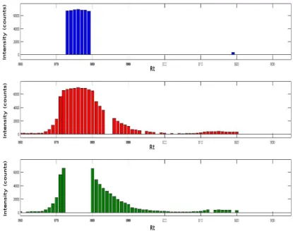
1.6 An isotopic cluster (proteomic data acquired on a low-resolution spectrometer) as it is visualized in a D map from [3]. The x-axis and y-axis of this noise-filtered 2-D map represent the chromatography and MS dimensions, respectively. Relevant mass spectrum and mass chromatogram are represented as cross-sections. A contour plot of the 2-D map is shown in the inset. . . 13

(20)

xviii LIST OF FIGURES

2.1 A high level flow chart of the MetAssimulo algorithm. . . 23

2.2 (a) Real normal urine 1_{H-NMR spectrum, (b) Mean of simulated normal urine} 1_{H-NMR spectra produced using MetAssimulo.} _{. . . .} ₃₁

2.3 (a) Mean simulated normal urine 1_{H-NMR spectrum, (b) Mean simulated} 1 H-NMR spectrum of urine in paraquat poisoning produced using MetAssimulo. . 34

2.4 (a) PCA scores plot of the first two principal components for the simulated nor-mal and diseased datasets show clear separation, (b) Loadings on PC1 indicating metabolite resonances that describe a large portion of the difference between the normal and diseased datasets, (c) Loadings on PC2 indicating metabolite that has a large within-group variance. . . 34

2.5 Simulated1_{H-NMR spectral peak shift for the two aromatic singlets of histidine.} ₃₅

2.6 Correlation matrix used to demonstrate MetAssimulo correlation functionality. . 35

2.7 Inter and intra-metabolite correlations: (i) Complete correlation matrix and in-sets (ii)-(v) showing strong negative inter-metabolite correlation between citrate and creatinine and positive between 2-oxoglutarate and creatinine (ii),(iii) and strong positive intra-metabolite correlations for creatinine (iv) and citrate (v). Colour scale indicates the level of Pearson correlation. . . 35

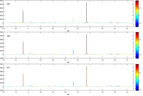
2.8 Pairwise correlation coefficients mapped as a colour code onto the mean spec-trum. Correlations to (a) citrate 2.65ppm, (b) creatinine 4.08ppm, (c) 2-oxoglutarate 2.44ppm. . . 36

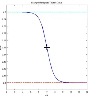
3.1 An example monoprotic titration curve modeled by the Henderson Hasselbach Equation is shown in blue. ThepKavalue is 7 and the inflection point is indicated with a black cross. The acid and base asymptotic limits are given by cyan and red dashed lines respectively. . . 39

(21)

LIST OF FIGURES xix 3.2 An example polyprotic titration curve model for a two site molecule is shown

in blue. The pKa values are 3 and 8 with the inflection points indicated by black crosses. The acid/base asymptotic limits are given by cyan, green and red dashed lines. . . 41

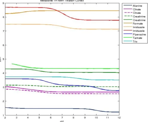
3.3 Metabolite 1_{H NMR titration curves showing varying effects of pH on several} different labelled metabolite resonances. . . 47

3.4 Metabolite 1H NMR titration curve for Imidazole 1 (a one site molecule with

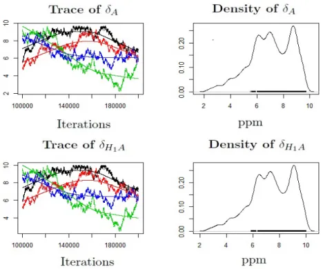
pKa = 6.95) . . . 49 3.5 MCMC trace and density plot for pKa of Imidazole using 1 site model. 4 chains

run with 100,000 iterations after a burn-in of 100,000 and thinning parameter of 10. . . 49

3.6 MCMC trace and density plot for acid and base limits of Imidazole using 1 site model. 4 chains run with 100,000 iterations after a burn-in of 100,000 and thinning parameter of 10. . . 50 3.7 MCMC trace and density plot for acid and base limits of Imidazole using 1

site model. 4 chains run with 500,000 iterations after a burn-in of 500,000 and thinning parameter of 100. . . 51

3.8 MCMC trace and density plot for acid and base limits of Imidazole using 1 site model with prior N(5,1)I(0,10). Multiple chains run for 100,000 iterations after a burn-in of 100,000 and thinning parameter of 10. . . 51

3.9 MCMC trace and density plot for acid and base limits of Imidazole using 1 site model with prior N(5,1)I(0,10). Multiple chains run for 500,000 iterations after a burn-in of 500,000 and thinning parameter of 50. . . 52

3.10 MCMC trace and density plot for acid and base limits of Imidazole using 1 site model with prior N(5,2)I(0,10). 4 chains run for 100,000 iterations after a burn-in of 100,000 and thinning parameter of 10. . . 53

(22)

xx LIST OF FIGURES

3.11 MCMC trace and density plot for pka of Piperazine using 2 site model. 4 chains run for 100,000 iterations after a burn-in of 100,000 and thinning parameter of 10. . . 54

3.12 MCMC trace and density plot for acid and base limits of Piperazine using 2 site model. 4 chains run for 100,000 iterations after a burn-in of 100,000 and thinning parameter of 10. . . 55

3.13 MCMC trace and density plot for acid and base limits of Piperazine using 2 site model with stronger prior N(5,2)I(0,10). 4 chains run for 100,000 iterations after a burn-in of 100,000 and thinning parameter of 10. . . 56

3.14 Polyprotic model fit for 1 Site molecule Formate (top), 2 Site molecule Creatinine (middle) and 3 Site molecule Citrate (bottom). Model1, Model2 and Model3 are polyprotic models withq= 1,2,3 sites respectively shown from left to right. The data is shown in blue, the fit and 95% credible intervals are indicated by black lines. . . 60

3.15 nlinfit model fit for 1 Site molecule Formate (left), 2 Site molecule Creatinine (middle) and 3 Site molecule Citrate (right) with data given in blue and the fit shown in black. The fit is so close as to be barely distinguishable by eye. . . 60

4.1 Examples of two commonly used wavelet functions (a) Daubechies 4, (b) Symm-let 8 [4] . . . 71

4.2 (a) Identified Peaks in m/z domain with SNR >3, (b) CWT coefficients of the signal at different scales, (c) ’Ridge Lines’ constructed from joining the location of local maxima at different scales and indicate where ’important’ features persist over multiple scales.[5] . . . 75

(23)

LIST OF FIGURES xxi 4.4 Plot of test data (red), posterior mean of distribution within each partition

(blue), marginal posterior probability of each data point being a change point (green line) and those points with a Bayes Factor>10are represented by dots at the top of the diagram. . . 90

4.5 Figure shows the signal data modelled (blue scatter plot), the marginal posterior probability of each data-point being a change point (red line plot) correctly indicating the change points, trace plot of K over the run (blue line plot) and the posterior distribution of K (blue histogram). The run was 6,000 iterations long including 5,000 burn-in. Prior mean on θ was 20 and initial value of K was set to 20. Prior parameters p and q were set to 0.5 and 20 respectively and prior parameters d and s were set to 50 and 20 respectively. Despite the data being noisy, the model converges quickly to the correct answer. . . 91

4.6 Figure shows the signal data modelled (blue scatter plot), the marginal posterior probability of each data-point being a change point (red line plot) correctly indicating the change points, trace plot of K over the run (blue line plot) and the posterior distribution of K (blue histogram). The run was 6,000 iterations long including 5,000 burn-in. Prior mean on θ was 20 and initial value of K was set to 20. Prior parameters p and q were set to 0.5 and 20 respectively and prior parameters d and s were set to 50 and 20 respectively. Despite there being relatively few data-points, the model again converges quickly to the correct answer. 92

(24)

xxii LIST OF FIGURES

4.7 Figure shows the signal data modelled (blue scatter plot), the marginal posterior probability of each data-point being a change point (red line plot) correctly indicating the change points, trace plot of K over the run (blue line plot) and the posterior distribution of K (blue histogram). The run was 10,000 iterations long including 5,000 burn-in. Prior mean on θ was 20 and initial value of K was set to 20. Prior parameters p and q were set to 0.5 and 20 respectively and prior parameters d and s were set to 50 and 20 respectively. Given there was considerable noise and few data-points, the model took slightly longer to converge but still did so relatively quickly and to the correct answer. . . 93

4.8 Sensitivity Analysis for prior parameter (a) p and (b) q on k indicating that increasing variance for prior on k allows greater number of change points to be fitted. . . 94

4.9 Sensitivity Analysis for prior parameters (a) d and (b) s indicating that increases of d or s correspond to higher mean and variance allowing greater variability of intensity within each partition and so fitting fewer change points. . . 95

4.10 Shows the real data (red) overlaid with the posterior mean (blue) and the marginal probability of a change point (green). Blue dots indicate points with a Bayes Factor >10. The inset shows a close-up of a relatively low intensity peak. 96 4.11 An example Total Mass Spectrum (with zoomed inset) showing raw data in black

and the wavelet-smoothed data in red. . . 98

4.12 Candidate peaks accepted by smoothing spline shape test using (a) Gaussian model and (b) Exponentially Modified Gaussian model. Blue circles indicate raw data points, red line indicates Gaussian fit, black line indicates EMG fit and green line indicates smoothing spline fit. . . 101

(25)

4.13 A 3-Hydroxycinnamic Acid peak intensity plot (a) of the raw data, with the colour scale indicating intensity and bin edge locations shown for H-MS (red lines) and apLC-MS (cyan lines). Also plotted are chromatograms of the H-MS bin (b) and the two apLC-MS bins (c, d). . . 111 4.14 A Creatine peak intensity plot (a) of the raw data, with the colour scale indicating

intensity and bin edge locations shown for H-MS (red lines) and apLC-MS (cyan lines). Also plotted are chromatograms of the H-MS bin (g) and the five apLC-MS bins (b-f). . . 112 4.15 Raw intensity plots, with colour scale indicating intensity, of 6 detected

metabo-lite peaks. Peak parameters shown for H-MS (red) and centWave (black) as boxes. (a) 4-Aminohippuric acid gives an example of centWave excluding high intensity data-points but H-MS captures the whole peak. For 3-Hydroxycinnamic acid in (b) we see a substantial drift in m/z value within a peak. H-MS includes all of the peak, whilst centWave detects two separate peaks. (c) Pimelic acid demonstrates where H-MS has defined a tighter area than centWave, including less noise. (d) Xanthine and (e) Riboflavin shows where H-MS excludes some relatively high intensity data-points that are captured by centWave. In (f) H-MS includes some lower intensity datapoints surrounding the Isocitric acid peak which perhaps should not be included as per the centWave parameters. . . 114 4.16 Intensity curves for all peaks detected by both a) H-MS and b) centWave across

the entire dilution series. The legend gives the molecule names, with the number in front indicating the replicate sample (1, 2 or 3). Strong linear trends give confidence that metabolites have been accurately identified and matched. . . . 116 4.17 Intensity curves for all peaks detected by either H-MS, a) with closeup b), and

centWave only, c) with closeup d), across the entire dilution series. The legend gives the molecule names, with the number in front indicating the replicate sample (1, 2 or 3). Lack of linear trend may be due to ion suppression or saturation effects. . . 116

(26)

4.18 Raw intensity plots, with the colour scale indicating intensity (ion count) at a particular data point, of (a) Hippuric acid-d2+H peak detected by both H-MS and centWave in replicate 1, (b) acetylcarnitine-d3+Na peak detected by centWave in replicate 1 and (c) 2-acetylcarnitine-d3+H peak detected by H-MS in replicate 2. Peak output parameters shown for H-MS (red) and centWave (black) as boxes. . . 117

(27)

Chapter 1 Introduction

1.1 Metabolomics

In the post-genomic era there has been a massive growth in ‘omics’ techniques investigating different levels of biological organisation. At the core of systems biology research is metabolic profiling, commonly known as metabolomics. Metabolomics focuses on high-throughput identi-fication and quantiidenti-fication of metabolites, small molecules (≤1500Da) involved in metabolism [6]. When attempting to relate genes to the overall function of a system, the metabolome (the complete set of metabolites of an organism) more closely reflects the activities of the organism at a functional level than, for example, the transcriptome [7]. Metabolic fluxes are not only regulated by gene expression, but also by additional factors, which include the abundance of metabolites as substrates (molecules acted upon by enzymes) and products (the output of a re-action or process) [8]. Therefore metabolic profiling adds another dimension to our understand-ing of biological systems. Figure 1.1 illustrates, somewhat simplistically, how metabolomics fits into the ‘omics’ structure of systems biology. In reality, the interactions between omics are not one-way only and much research is devoted to understanding the complex ’inter-omics’ mechanisms in order to build up a holistic view of an organism’s function. The omics research areas mentioned here are by no means an exhaustive list and the depth and breadth of omics

(28)

2 Chapter 1. Introduction

specialities is continuously expanding.

Genomics → Transcriptomics → Proteomics → Metabolomics (1.1)

With the relatively recent development of systems biology comes the promise of ‘personalised health-care solutions’ and an improved understanding of molecular epidemiology [9]. The ap-plications of accurate metabolic profiling reach from studying drug toxicity and pharmacology to disease-screening for conditions such as diabetes or cancer [10, 11, 12, 13, 14]. Metabolomics, as an expression of genetic and environmental factors, is key to furthering our knowledge of how humans and other organisms function as individuals and interacting complex systems. There are generally considered around 2000 major metabolites for humans, however this number increases significantly when secondary metabolites are explored [15, 16]. Although the terms ‘metabonomics’, ‘metabolomics’, metabolic ‘fingerprinting’ or ‘profiling’ were assigned subtly different definitions originally, they are usually used interchangeably today. Metabolomics can be formally defined as ‘the comprehensive quantitative analysis of all the metabolites of an organism or specified biological sample’, typically involving ‘the quantitative measurement of the multi-parametric time-related metabolic responses of a complex (multi-cellular) system to a pathophysiological intervention or genetic modification’ [9].

1.2 Technologies

Metabolomics lacks a definitive data-acquisition technique, with a variety of methods offering different advantages and disadvantages depending on the aims or priorities of a study or ex-periment. However, the two main techniques for capturing metabolite data are 1H Nuclear Magnetic Resonance (NMR) Spectroscopy and Mass Spectrometry (MS) [17, 18]. Metabolites in biofluids are in dynamic equilibrium with those in cells and tissues so their metabolic profile reflects changes in the state of an organism due to disease or environmental effects. NMR is highly reproducible, offering the advantage of being non-destructive, and is able to give a nearly global metabolite profile including structural information enabling the identification of

(29)

1.2. Technologies 3 the most abundant metabolites. MS boasts a significantly superior sensitivity [19, 17], but has great variability of results as consequence which is exacerbated by time-consuming and error-prone sample preparation procedures. There are efforts under way within the metabolomic community to marry the merits of both NMR and MS and forge a multi-platform approach to metabolomics research [20, 21, 22]. Whilst NMR spectra are typically characterised by a 1-dimensional signal whose intensity varies in proportion to metabolite concentrations detected across a scale of ‘parts per million’ (ppm) of an internal standard, MS is usually paired with a chromatographic technique such as liquid or gas chromatography (LC-MS or GC-MS [23]) resulting in a 2-dimensional dataset of intensities varying in both retention time (Rt) and along the mass-to-charge ratio scale (m/z). Metabolites present as ‘peaks’ in the data, where the instrument has registered the presence of a molecular species within the biofluid. NMR ma-chines are typically more expensive with faster running time, but LC-MS mama-chines certainly have more widespread availability. Use of GC-MS has largely been superseded by LC-MS due to more convoluted sample preparation, limitations on the size and type of molecules that can be measured as well as slow speed of data acquisition. Despite this, GC-MS is still used in plant metabolomics.

1.2.1

1

H Nuclear Magnetic Resonance Spectroscopy

1_{H-NMR spectroscopy gives an almost global metabolic profile as it has the potential to detect} nearly all proton-containing metabolites and allows metabolites to be detected simultaneously without pre-selection. Biofluids contain thousands of metabolites, but a typical NMR spec-trum will only contain signals from a few hundred of the most abundant metabolites. Despite relatively poor sensitivity in comparison with analytical methods such as mass spectrometry, NMR spectroscopy requires minimal sample preparation meaning the process is highly repro-ducible, and is able to measure concentrations as low as 100µM [24] and even lower with recent techniques such as cryoprobe technology [25]. NMR spectroscopy utilises the fact that under a magnetic field, the atomic nuclei (in this case,1_{H) absorb at a frequency proportional to the} strength of the field, by detecting the resonance of hydrogen nuclei. When placed in a magnetic

(30)

field, the magnetic moment of the hydrogen atom adopts one of the two permitted orientations of different energy. The difference in energy of these two states depends on the strength of in-teraction between the magnetic moment of the nucleus and the field [26]. This energy difference can be measured by applying electromagnetic radiation of a certain frequency which causes the nuclei to shift between states. ‘Chemical shift’ is defined as the effect of the chemical structure of the molecule on the resonance frequency of the nuclei. Therefore the NMR spectrum for each metabolite is comprised of a characteristic pattern of peaks or resonances, derived from three main factors:

1. The chemical shift (δ) of each resonance is dependent upon the local magnetic field ex-perienced by each nucleus. This local field is dependent on the degree to which molecular orbitals shield the influence of the external spectrometer field. Thus the chemical shift re-flects the chemical structure and bonding configuration of the metabolite. Whilst Hz is the fundamental energy unit of NMR, the frequency reported is dependent on the magnetic field strength so the position of each peak is measured relative to that of an internal standard and given in a scale of parts per million (ppm) instead [26]. A commonly used internal standard is 3-(Trimethylsilyl)-Propionic acid-D4 (TSP).

2. Spin-spin coupling (also known as scalar coupling or J-coupling) is the phenomenon of magnetic interactions between nearby nuclei. This means a proton has more than one resonant frequency resulting in a juxtaposition of peaks called a ‘multiplet’ as shown in Figure 1.1, with the pattern determined by the chemical structure of the molecule.

(31)

1.2. Technologies 5 3. Integrated peak area for a given metabolite is proportional to the number of observed 1H nuclei (assuming there are no differential relaxation effects) and allows quantification of the metabolite concentrations.

The resulting dataset consists of a series of resonance intensity measurements taken over a grid of frequencies, with the x-axis corresponding to the resonant frequency (usually plotted to increase from right to left) and the y-axis gives the resonance intensity (see Figure 1.2). The spectrum of a pure compound will consist of a ‘signature’ of peaks reflecting the factors described. Under ideal conditions, each peak takes the form of a Lorentzian curve, represented by the following equation:

lγ(x) =

2γ

π(4x2 ₊_γ2₎ (1.2)

where γ is referred to as the ‘linewidth’ (or ‘peak-width at half-height’). The NMR spectrum

Figure 1.2: A typical1H NMR spectrum of a human urine sample with some labelled metabolite resonances, where the x-axis is ppm (parts per million) relative to some internal standard and the y-axis gives the signal intensity.

of a complex mixture can be well approximated by a linear combination of the spectra of pure compounds, i.e a biofluid spectra containing K different metabolites can be treated as

K-dimensional objects, in which each dimension represents the concentration signal of a single metabolite [27]. This superposition of peaks and multiplets results in a complex spectrum of overlapping signature patterns. These spectra can be further complicated by peak positional variation, due to matrix effects or differences in experimental conditions as well as variation in the chemical properties of the sample, e.g pH value and the strength of other ionic species in the

(32)

mixture [28]. These problems, along with background noise and the presence of contaminants, make peak identification very difficult particularly for automated algorithms.

Pre-processing is typically performed to provide a dataset that is more informative for sta-tistical modelling. The data is usually transformed into a matrix of m variables (metabolite concentrations or metabolic signals) bynsamples. This may be achieved by first identifying in-dividual metabolite signals and quantifying them (both non-trivial tasks), or by ‘binning’ (also referred to as ‘bucketing’) the spectra into equal regions (typically 0.04ppm wide). Binning is often preferred to using the entire chemical shift resolution as not only does it reduce the dimension of the data, but may also limit the effect of peak positional variation. Alternatively, variation in peak position can be reduced by using an alignment procedure [29]. Normalisation of the matrix rows may be performed with the aim of removing variation between samples by multiplying by a constant. The samples may be normalised relative to an internal standard or the total integrated intensity across the spectrum, depending on whether it is more impor-tant to determine absolute or relative levels of metabolite concentrations. Another option is to normalise the spectra with respect to a selected ‘reference’ spectra using probabilistic quotient normalisation or histogram normalisation for example, but knowledge of the biological context of the data is essential when choosing a normalisation method [30, 29]. Sometimes the columns of the data matrix will also be scaled, allowing more emphasis to be placed on low intensity signals. Variables are often scaled to unit variance, or alternatively Pareto or Log scaling may be used [25]. Another typical pre-processing step is to remove the spectral region worst affected by the unwanted water signal, since suppression of these large resonances is usually imperfect. The next step in the statistical analysis of metabolic NMR data is to perform both unsupervised (exploratory) and supervised (e.g. classification/regression) analysis, with the aim of identifying and characterising important differences between classes resulting from the presence of external or internal stimuli to the organism. Classical methods (employed in metabolomic analysis across technologies) include Principle Components Analysis (PCA) and Partial Least Squares (PLS) regression, which aid interpretation of the data by projecting onto lower dimension spaces corresponding to either the highest variance, or highest covariance between the scores of the data and the response variable. Typically the analysis workflow will include firstly unsupervised

(33)

1.2. Technologies 7 clustering such as PCA and then be followed by a supervised method (PLS-DA etc.) to enhance this separation and understand which variables are responsible for the differences between datasets.

PCA is a useful exploratory analysis tool. PCA transforms a dataset consisting of observations of several variables into a set of orthogonal ’principal components’. The principal components are ordered in such a way that the first accounts for the as much variance in the data set as possible and the last accounts for the least, whilst maintaining orthogonality between the components. PCA scores correspond to a linear combination of the original variables and can be defined as the transformed variable values corresponding to a particular data point. Loadings describe the weight that each original variable contributes to the component score. Usually, the dimensionality of the problem is reduced by considering only the first two or three principal components as they will typically account for most of the variability of the data. This technique is particularly relevant for metabolomics given the original variables are highly collinear.

PLS is a broad class of techniques for modelling relations between variable sets using latent vari-ables. Generally speaking PLS creates orthogonal score vectors (or components) that maximise covariance between different sets of variables by projecting both the predictors and outcomes to a new space. It is particularly useful when the variables outnumber the observations and are highly collinear. Whilst PCA chooses the x-axis scores to explain as much factor variation as possible, PLS chooses x and y scores so that the relationship between successive pairs of scores is as strong as possible as expressed by covariance of scores. As such, PLS scores reflect the covariance structure between predictors and response, with the aim being to maximise covari-ance between the response variable and component scores. Extensions of these methods, for example PLS regression, Orthogonal (O/O2-PLS) PLS and Discriminant Analysis (PLS-DA), are also used throughout the metabolomic community. Alternative approaches include Sup-port Vector Machines, Genetic Algorithms and Programming, kernel methods and tree-based classifiers (e.g. Random Forests) [30, 25].

Statistical Spectroscopy is a collection of tools that has been rapidly expanding since the de-velopment of Statistical Total Correlation Spectroscopy (STOCSY) [31]. STOCSY utilizes

(34)

correlation analysis to construct a pseudo-2D spectrum providing useful information on cor-related metabolic signals in 1_{H NMR. This is useful for identifying signals belonging to the} same compound (some molecules have more than one signal for each measurement) as well as highlighting correlated metabolites which may be part of the same metabolic pathway. The methods used by STOCSY have now been extended to tackle analysis across other technologies, for example Statistical Hetero-Spectroscopy (SHY) aims to incorporate information obtained using MS data [32]. 2D-NMR methods employing an additional NMR nuclei, e.g. 13C, are often used similarly in metabolomic analysis with the advantage of providing further informa-tion useful in elucidating the chemical structure and identifying unknown molecules, as well as signal dispersion in the additional dimension [33].

Identification of metabolite signals present in NMR data is greatly aided by the development of several databases dedicated to documenting metabolite data. Two of the largest are the Biological Magnetic Resonance Bank (BMRB) [34] and the Human Metabolome Database (HMDB) [35]. Although the BMRB includes information on molecules including peptides, proteins, and nucleic acids, the HMDB focusses specifically on small molecule metabolites found in the human body. Whilst these databases are valuable tools, there exist several challenges in curating the ‘ideal’ data resources. Two major problems are the unknown abundance of unknown metabolites within the human metabolome meaning the databases are inherently limited in their coverage, and also the relevance of acquisition conditions, for example there may be much variation in pH, use of solvents etc for different metabolite data. In addition to the metabolite databases for particular technologies there are useful resources linking metabolites to particular pathways, for example Kyoto Encyclopedia of Genes and Genomes (KEGG) [36], MetaCyc [37] and ConsensusPathDB [38].

The methods for processing and interpreting metabolic 1_{H NMR data are many and varied.} In Chapter 2, a package for simulating human urine 1_{H NMR metabolic profiles is introduced,} whilst Chapter 3 tackles the problem of modelling pH-induced peak positional variation.

(35)

1.2. Technologies 9

1.2.2 Liquid Chromatography - Mass Spectrometry

Most biologically interesting chemicals are present as isomers: molecules having exactly the same mass but a different structure. Using a separation technique, such as chromatography, before using mass spectrometry can help tackle this problem by further dispersing the signal in an additional dimension. Another advantage of separation is that it limits the amount of analytes being ionized simultaneously and thus reduces the possibility of ion suppression effects. Ion suppression can also be a result of the sample matrix used and is unpredictable, impairing detection capability, quantification and reproducibility [39, 40]. After elution, the mobile phase

Figure 1.3: A high level view of the LC-MS workflow taken from [1]. The sample enters the liquid chromatography where compounds are separated in the time domain, then the sample is ionized and passed to the mass spectrometer where compounds are further separated by their mass. This results in a 2-dimensional dataset where signals are described by a (retention time (Rt), mass-to-charge ratio, intensity) triplet.

passes through an interface before moving to the mass spectrometer. This interface either attempts to remove the mobile phase, or pumps the solution straight into the mass spectrometer in order to minimize contamination. Figure 1.3 illustrates the LC-MS work-flow.

Liquid Chromatography works by pumping a ‘mobile phase’ solution through the ‘stationary phase’ or ‘column’, where the time taken from injection to elution at the detector is dependent on the interaction between the analyte and the mobile and stationary phases. The mobile phase is a solution containing the sample and any solvents or buffers used. Solvents are used in order to control the strength of interaction different molecules have with the chromatographic column, whilst buffers manage the degree of ionization of the analyte. Even high-purity solvents

(36)

and buffers can contribute contaminant signals to background noise. The mobile phase is then delivered into the column under high pressure in order to sustain a constant flow rate and thus ensure reproducibility. Separation occurs when elements of the sample mixture interact to different extents with either or both of the mobile and stationary phases and so take different amounts of time to traverse the column. There are many different configurations of column and mobile phases that give widely varying results depending on the physiochemical properties of the molecules analysed [41]. Gradient elution, for example, actually varies the composition of the mobile phase during the experiment in an attempt to achieve higher resolution separation. LC technology is fast evolving and advances in methodology means that the peak capacity of a single scan is ever-increasing. HPLC (High Performance Liquid Chromatography) has been a widely used technique since the 1990s. HPLC utilises the fact that employing smaller particles for the stationary phase of the column and injecting the mobile phase at high pressure increases both the speed of elution and the number of peaks resolved per unit time in gradient separations, resulting in both improved sensitivity and resolution. More recently UPLC (Ultra Performance Liquid Chromatography, pioneered by Waters MS Technologies, Ltd., Manchester, U.K.) has become the fore-running technique using yet smaller particles to improve performance even further. The enhanced resolution and sensitivity means that run times are quicker and reproducibility is better than for normal HPLC.

Mass spectrometers differentiate compounds within a complex mixture by measuring their molecular mass-to-charge ratio. Upon entering the mass spectrometer, the sample is ionized using one of a variety of techniques : electron or chemical ionization, fast-atom bombard-ment (FAB), thermospray (TSP), electrospray (ESI) etc, with ESI the most commonly used in metabolomics. ESI is a relatively ‘soft’ ionization technique that causes minimal fragmentation and can be run in positve and negative modes in order to capture both sets of analytes. Then, ions of different mass-to-charge ratios (m/z) are separated and the counts of each group of ions is measured. There are several different methods for mass analysis, for instance Quadrupole Mass Analysers vary the voltage between two pairs of rods in order to bring ions of different m/z to the detector as required. This instrument has high sensitivity for targeted analysis [42]. Another type of mass analyser common within metabolomics is Fourier Transform Ion

(37)

1.2. Technologies 11 Cyclotron Resonance (FT-ICR), which determines the m/z value based on the cyclotron fre-quency (dependent on mass) of the ions trapped in a fixed magnetic field. The signal is Fourier Transformed to the frequency domain in order to calculate the mass spectrum [43]. FT-ICR has a very high mass accuracy so is particularly useful for identifying unknown analytes. Per-haps the simplest mass separation device is the Time-Of-Flight (TOF) analyser. The ions are first accelerated by an electromagnetic field. TOF then utilizes the fact that regardless of the ionization technique, all the ions are given the same kinetic energy meaning that the velocity of each is inversely proportional to the square root of its mass. Thus, the m/z of the ion can be deduced according to how long the ion takes to traverse the flight tube of the instrument [42]. Due to its simplicity and fast scanning capability, TOF is being used increasingly in LC-MS instrumentation to produce high-resolution spectra for untargeted applications.

Mass analysers can also be run in tandem with an alternative mass analyser (or indeed more than one), for example QTOF mass analysers combine the strengths of Quadropole mass anal-ysis with those of Time-Of-Flight analanal-ysis simultaneously to improve sensitivity and accuracy. These tandem mass spectrometers can also be used to produce additional structure information about compounds by fragmenting ions and identifying the fragments. The Quadropole analyser may be used to select a mass range which is then measured by the TOF, or alternatively for fragmenting ions which are then detected in the TOF analyser.

The whole process results in a 2-dimensional data set: an intensity for each retention time (Rt) and mass-to-charge ratio (m/z) pair, as shown in Figure 1.4 [42, 44]. Metabolite quantification relies on the fact that peak intensity (or peak volume) is usually proportional to the concen-tration of a molecule [45]. A ‘mass spectrum’ is defined as the ions detected for one particular retention time value, i.e. a slice in the retention time dimension, whilst slicing at constant m/z gives a ‘chromatogram’ (Extracted Ion Chromatogram or EIC) for each m/z value. In constructing chromatograms, one can either use the maximum intensity (resulting in a ‘Base Peak Chromatogram’) or the total intensity at each Rt point in the slice (EIC). However, com-plications arise in defining a m/z ‘bin’ for each chromatogram since there can be drift in the measurement of m/z (see Figure 1.5) and this problem will be examined more closely in Chapter 4. The characteristics of peaks in the m/z direction or ‘MS peaks’ are largely determined by the

(38)

Figure 1.4: A 2-D Intensity map of LC-MS Data from [2]. x and y axes give the Retention Time (Rt) and mass-to-charge ratio (m/z) and z axis gives the intensity (ion count) detected.

Figure 1.5: A chromatographic peak split across three bins due to drift in m/z.

instrument used. Gaussian curves are commonly used for MS peak modelling, although other shapes may perform better [23]. The LC peak shape is dependent on a complex interaction of factors, not entirely understood, such as solvent concentration, separation gradient etc. Again, many use a Gaussian curve for simplicity [46, 47], but it is acknowledged that peaks usually have a long tail and are sometimes even bi-modal [41, 48]. Chromatographic peaks often re-quire alignment between successive samples due to the difficulty ensuring the reproducibility of the process resulting in non-linear distortions of the Rt axis. The chromatographic domain

(39)

1.2. Technologies 13 is usually used in order to discriminate between analyte and noise peaks [45].

The signal is complicated further by isotope patterns (often predictable if the compound iden-tity is known) due to the abundance of naturally occurring isotopes, such as C13_{. This means} multiple peaks may be registered for a single molecular species in mass spectra at different m/z locations. Figure 1.6 shows an example of protein MS. The mono-isotopic peak registers at (54.7s, 526.6m/z), and at least two well-defined smaller isotopic peaks are present at 527.5m/z and 528.3m/z. In addition to this, heavy molecules such as proteins may generate a group of related peaks with different charge states[41]. However, metabolites are relatively small by comparison (<1500Da) producing few, if any multiply charged ions so this is not generally a big problem within metabolomics [42]. Other complications include fragmentation of molecules

Figure 1.6: An isotopic cluster (proteomic data acquired on a low-resolution spectrometer) as it is visualized in a 2-D map from [3]. The x-axis and y-axis of this noise-filtered 2-D map represent the chromatography and MS dimensions, respectively. Relevant mass spectrum and mass chromatogram are represented as cross-sections. A contour plot of the 2-D map is shown in the inset.

during the ionisation process, resulting in a parent and correlated daughter ions being detected. Linking fragments (co-eluting peaks) using statistical post-processing techniques can be helpful in identifying unknown molecules. Sometimes dimerization can occur, where two molecules of the same species combine and so are detected as a single ion at twice the m/z value. Ionization can also result in adducts, for example protonated or deprotonated alkali metals binding

(40)

to-14 Chapter 1. Introduction

gether as well as neutral losses (water CO2 etc.) for metabolites. The mechanism behind this process is not fully understood but given the small size of metabolites adduct formation can significantly alter m/z values [49].

There exist numerous obstacles to overcome when interpreting LC-MS data. Tailing peaks can often be mistaken for multiple consecutive peaks, and quantification for one peak can contain contaminating information from a confounding overlap of signals [50]. This can be overcome somewhat by modelling the spectra as a sum of peaks, each represented in some parametric form and then performing deconvolution, but this can introduce new errors. The signal can be corrupted by ionization and ion-suppression effects, usually arising when polar contaminants are competing with the target analyte present for available ions, as well as by impurities from the buffers and solvents used [17].

Noise is usually characterized by high frequency, low intensity, narrow peaks, and is generally more prevalent at the beginning and end of elution. Most molecules elute with an intensity markedly greater than the expected level of noise, but molecules eluting with a low abundance makes them extremely difficult to identify. Feature detection is hampered further by non-linear drifts in retention time (and sometimes m/z values as mentioned earlier). In addition, aligning spectra across many samples is complicated by peaks that are missing or simply undetected in some samples, providing another huge challenge beyond the scope of this thesis [45].

Similarly to NMR there exist reference databases for MS spectra, such as MassBank [51] and METLIN [52]. However, since the between-sample variation of elution times for even the same instrument can be so large, no Rt index is currently available for LC-MS [53]. In adition to spec-tral library matching, a combination of techniques, such as NMR, are usually required to gain enough structural information to confirm a metabolite identity. Sample preparation method, choice and configuration of LC-MS instrumentats and algorithm/software employed for data processing can result in widely varying datasets even from the same sample. Pharmaceutical regulators are moving to introduce standard protocols in an effort to make results more stan-dardised and comparable (Metabolomics Standard Initiative) and use of pilot studies, internal standards, QCs and other ’quality assurance’ measures are widely used in order to tackle the

(41)

1.3. Bayesian Inference 15 issue of reproducibility and robustness of results.

1.3 Bayesian Inference

Both NMR and LC-MS require sophisticated statistical techniques in order to perform inference on the data obtained. Within statistics there are two main inferential frameworks: ‘frequentist’ and ‘Bayesian’. Frequentist inference is based upon the assumption that the observed data can be considered as one instance of a series of infinitely repeatable experiments [54] and standard frequentist methodologies include statistical hypothesis testing and calculating confidence in-tervals. Whilst frequentists tend to consider the probability of the observed data arising given a hypothesis, Bayesians are more converned with the probability of a hypothesis given the observed data. Bayesian inference is derived from Bayes’ Theorem (Equation 1.3):

p(θ|y, φ) = p(y|θ)p(θ|φ)

p(y|φ) (1.3)

where p(y|θ) is the likelihood of the data given the model parameters, θ is a parameter of the likelihood distribution with prior θ ∼ p(θ|φ), φ is a hyper-parameter of the distribution of θ,

p(y|φ) is the marginal likelihood:

p(y|φ) = Z

θ

p(y|θ)p(θ|φ)dθ (1.4) and p(θ|y, φ) is the posterior probability of parameter θ.

Practically speaking this means setting up a full probability model, conditioning on the ob-served data (y) in order to calculate the posterior distribution (the conditional probability distribution of the unobserved quantities of interest, given the observed data) and then evalu-ating the model fit [55]. Frequentist ‘results’ are usually true or false conclusions drawn from significance tests, whereas Bayesian results more often take the form of probability distributions for parameters that attempt to describe the data. Bayesian methodology is employed widely within metabolomics for a variety of different purposes, for example variable

(42)

selection/dimen-16 Chapter 1. Introduction

sion reduction, latent variables analysis, network/pathway analysis and spectral deconvolution among many others.

When practicing Bayesian inference, it is often useful to be able to calculate posterior estimates of characteristics of the model parameters. In the case of multi-parameter models, where θ = (θ1, ..., θk), this requires averaging over ‘nuisance’ parameters (parameters on which one is not concerned with performing inference). Supposing the parameter of interest isθ1, the conditional distributionp(θ1|y) must be derived from the joint posterior distributionp(θ|y) = p(θ1, ..., θk|y). Averaging over the nuisance parameters gives:

p(θ1|y) = Z θk ... Z θ2 p(θ1, ..., θk|y)dθ2...dθk (1.5) or alternatively p(θ1|y) = Z θk ... Z θ2 p(θ1|y, θ2, ..., θk)p(θ2, ..., θk|y)dθ2...dθk (1.6) However, these posterior distributions are often high dimensional and very difficult to calculate either analytically or numerically. The problem of making inferences on this type of distribution is addressed by using Markov Chain Monte Carlo (MCMC) methods. MCMC enables simula-tion of random draws from a complex probability distribusimula-tion, say f(x). MCMC methods are based on Markov Chains, which are stochastic processes Xt, t= 0,1,2, ...such that:

P(Xn =xn|X0 =x0, ..., Xn−1 =xn−1) = P(Xn=xn|Xn−1 =xn−1) (1.7) i.e. the current observation only depends on the previous one and not the entire observation history [54]. MCMC methods essentially involve constructing a Markov Chain whose target distribution is the distribution of interestf(x). Once a large enough sample has been simulated, the functionals of interest can be calculated to any degree of accuracy.

There are numerous methods for building the required Markov Chain. For example Metropolis-Hastings uses a ‘proposal distribution’ q(x) to propose a candidate value Y for Xt+1, possibly

(43)

1.3. Bayesian Inference 17 depending on Xt, and accepts it with probabilityα(Xt, Y) where

α(Xt, Y) =min(1,

f(Y)q(Xt|Y)

f(Xt)q(Y|Xt)

) (1.8)

and f(x) is the function of interest. A special case of the Metropolis-Hastings is the Gibbs sampler. Suppose draws ofθ= (θ1, ..., θk) must be obtained from the joint distribution function

f(θ1, ...θk). Then for each drawt = 1,2, ..., eachθ (t)

i is sampled from the conditional distribution given by p(θ_i(t)|θ₁(t), ..., θ(t)_i−1, θ(t−1)_i+1 , ..., θ_k(t−1)) (proportional to the joint distribution) so that each variable is sampled using the most recently updated values of the other variables. There are many variations on these samplers, so-called ‘adaptive’ modifications aimed to increase the sampling efficiency of the algorithms.

A ‘burn-in’ period is usually utilised (i.e. the first M iterations are discarded) as we accept we are unlikely to choose good starting conditions and thus the initial estimates are likely to be poor. Thinning is the practice of saving only every n-th iteration sometimes with the aim of speeding up post-processing or reducing required memory but also as an attempt to remove auto-correlation. For example, to obtain a run of 10,000 iterations one would run n×10,000 simulations and save only every n-th one. However it has been argued that if the entire chain is long enough, the auto-correlation has likely averaged out anyway and thinning provides little additional benefit to this end [56].

Convergence of MCMC is a major concern for Bayesian statisticians with the parameters es-timated often correlated with themselves over the iterations or with each other making con-vergence slow and difficult to execute. Despite much theoretical research into concon-vergence computations, there is limited benefit thus far for practical applications. Although it remains impossible to be certain that your MCMC sample is truly representative of the target distri-bution, there are many diagnostic measures and techniques to help somewhat evaluate success. Indeed Cowles and Carlin provide thorough reviews of these[57].

One of the simplest checks is visualisation of how well your chains are ‘mixing’ or moving around the sample space. Plotting traces (parameter value vs. iteration number) can show

(44)

you if your parameter gets stuck or moves poorly. ‘Running mean plots’ (plotting the sample mean up to each iteration vs. iteration number) can also be useful to this end. Investigating the auto-correlation can also provide clues as to the convergence of your chain. A ‘k-th lag auto-correlation’ can be computed and we would expect the correlation to decrease as the lag increases. Persistently high auto-correlation for high k is again indicative of poor mixing.

One commonly used convergence diagnostic is the ‘Gelman and Rubin Multiple Sequence Di-agnostic’ which is calculated using multiple chains per parameter. Consider the ‘potential scale reduction factor’: ˆ R = s ˆ V ar(θ) W (1.9)

where V arˆ (θ) is the estimated variance of the target distribution as a weighted average of the within-chain, W, and between-chain, B, variances:

ˆ

V ar(θ) = (1− 1

n)W +

1

nB (1.10)

When ˆR is high (> 1.1 or so) this indicates the chains should be run longer to improve con-vergence. A ‘Gelman plot’ shows how the potential scale reduction factor changes through the iterations and is another useful diagnostic.

There are several software packages available for automating the Bayesian analysis of models via MCMC methods. WinBUGS (arising from the BUGS - ‘Bayesian inference Using Gibbs Sampling’ project based in the MRC Biostatistics Unit at Cambridge, England) is one of the most popular [58]. It provides a framework for defining Bayesian hierarchical models and a library of sampling routines to perform inference. Several extensions have been developed allowing construction and analysis of ever more complicated models. One such alternative, JAGS (Just Another Gibbs Sampler), was developed with the objective of being an open-source engine for the BUGS language [59]. JAGS is highly extensible and allows users to develop new libraries and add-ons. Both WinBUGS and JAGS can interface to R, making them useful tools

(45)

1.4. Aims 19 in the arsenal of any Bayesian statistician. Whilst MATLAB was used extensively during the development of this thesis to write new algorithms, both WinBUGS and JAGS were used (via R) to perform Bayesian statistical analyses.

Bayesian methods are used throughout ‘omics’ analysis from processing and analysing NMR [60], LC-MS [61, 62] and GC-MS [63] data among others, to elucidating metabolic pathways [64]. Within metabolomics, particularly when modelling data that is driven by some complex physio-chemical reaction, the Bayesian framework allows us to incorporate prior knowledge of this underlying mechanism whilst allowing the observed data to speak to us about the other unknown interactions occurring that result in both structured and unstructured variability.

1.4 Aims

The major bottlenecks within metabolomics research can be broadly categorised as metabolite identification, data processing and interpretation of results. Metabolite identification depends on the robustness of the data capture, ability to match with standards and is complicated by the great variability of molecular structures and abundance. Data processing and reduction techniques are complex and often bespoke depending on the focus area of a given laboratory, meaning that different results can be produced from a single dataset by using alternative software or statistical methods hampering reproducibility and validation by different research groups. In addition to this, manufacturers’ processing software is often tied to their particular spectrometer, although open source software developers and researchers attempt to produce algorithms that perform competitively whilst being compatible with multiple machine types used across different labs. Further downstream in the data flow, all these issues greatly affect the ability to assign biological significance to experimental results, i.e. the ultimate aim of most metabolomic investigations. Given the complex nature of the numerous statistical challenges facing metabolomics research, this thesis sets out to tackle a few of these problems.

• In order to fulfil the need within metabolomics for simulated 1_{H-NMR data with which} to develop and test new techniques for statistical inference, Chapter 2 presents a novel

(46)

package ‘MetAssimulo’, designed to draw on data from the Human Metabolome Database (HMDB) and an NMR Standard Spectra Database (NSSD) in order to simulate realistic human urine spectra [65]. It also allows inclusion of peak shift and inter-metabolite correlations.

• Chapter 3 aims to further demystify 1_{H-NMR metabolic profile data by Bayesian} mod-elling of the relationship between pH and peak positional variation. Being able to estimate peak shift parameters would be of great use in the deconvolution of NMR spectra and also accurately simulating peak shift using MetAssimulo.

• In Chapter 4 I move on to the challenges faced in the processing of LC-MS data, taking a look at existing algorithms and the variety of techniques used. A Bayesian Change Point Model is also explored for this application. H-MS, a novel method for data-binning and peak detection, is described and its performance is compared to an adaptive technique apLC-MS [66] and a commonly used package XCMS [46].

(47)

Chapter 2 Simulation of Realistic

1

H-NMR

Metabolic Profiles: MetAssimulo

Metabolic NMR spectra are highly complex and the field benefits greatly from the application of machine learning and other statistical tools to extract information. Pattern recognition analyses such as Principal Components Analysis (PCA) have long been combined with NMR to investigate normal and pathological metabolic states [67]. Data processing methods are being developed to extract metabolite information and concentrations from raw spectra, allowing automation of spectral processing. Development of advanced mathematical, statistical and computational methods are also essential for characterisation of the metabolic state, delineation of metabolic changes over time and the efficient identification of potential biomarkers. There are a wide variety of diseases where key changes in metabolites have been deduced e.g. cancer, diabetes, hypertension etc. [68, 69, 14]. However, as algorithms and methods are developed, they need to be refined and validated to ensure results will be biologically meaningful. It is hard to effect this without using test datasets where the true answers are known; this can be accomplished using simulation techniques. An alternative approach is to design artificial mixtures of metabolites which are prepared and analysed in identical fashion to real samples. However this is expensive in terms of man power and instrument time, and offers few advantages over in silico simulation when assessment of analytical procedures is not required.

(48)

22 Chapter 2. Simulation of Realistic1_{H-NMR Metabolic Profiles: MetAssimulo} The purpose of MetAssimulo is to simulate datasets of realistic NMR spectra with known

parameters in order to test data analysis techniques, hypotheses and experimental designs. Few methods for generating simulated NMR datasets have appeared in the literature to date [70, 71]. Most model a limited number of metabolites, make no attempt to reproduce real-istic levels of metabolites, and do not allow for between-metabolite or ‘inter-metabolite’ cor-relations ([71] excepted) and do not always model peak positional shifts. It is common to fit Lorentzian peak shapes in an attempt to characterize spectral peaks, e.g [70]. However, this ignores the fact that peak shapes in real NMR profiles are variable and can be far from ideal. Here a novel approach is outlined: making use of individual standard metabolite data extracted from the Human Metabolome Database (HMDB) [35] and a local NMR standard spectra database (NSSD). Many metabolic profiling labs host their own NSSD appropriate to the biological systems and sample types they work with and thus the simulations can be tailored to virtually any sample type or organism as required. In this work human urine is used as the example biofluid as it is one of the most widely used in the field and, in healthy subjects, has no protein or lipid content, both of which make the simulation more complex. MetAssimulo is written in MATLAB with a graphical interface allowing the user to alter pro-cessing parameters and add new standard spectra as needed. The software is freely available along with an example NSSD of 48 metabolites commonly found in normal human urine (at

http://cisbic.bioinformatics.ic.ac.uk/metassimulo/). It must be stressed that this list of metabolites and their concentration means and standard deviations does not constitute a

definitive description of human urine; such a goal is beyond the scope of this chapter. It is provided for the sole purpose of demonstrating the capabilities of the software.

MetAssimulo was initially developed by a student Rebecca Jones. Rebecca worked on the first version of MetAssimulo able to simulate peak shifts. The author’s work built on this: bug fixes, incorporating metabolite correlations, extracting data from the HMDB and increasing efficiency which required a substantial amount of recoding. This chapter is based on the MetAssimulo article published in BMC Bioinformatics [65].

(49)

2.1. Implementation 23

2.1 Implementation

MetAssimulo performs various functions accessed though the Graphical User Interface (GUI): pre-processing the pure spectra, simulating metabolite concentrations, incorporating peak shifts and creating the final mixture spectrum, shown in Figure 2.1. By default it produces two groups of spectra based on different metabolite mixtures; these could represent controls (normal) and cases (diseased) subjects. Each metabolite has a characteristic pattern of peaks on a linear

Figure 2.1: A high level flow chart of the MetAssimulo algorithm.

scale, the chemical shift, given by δ in ppm. The signal intensity, y(δ), in a spectrum of metabolites k= 1, .., K (whereK is the total number of metabolites in the mixture) at a given

δincreases proportionally to the concentration of each metabolite,ck, present in the sample and their number of observed protons, pk. The different metabolite spectra are summed together to produce the overall mixture spectrum. Normally distributed additive noise(δ)∼N(0, σ2) (see