Development of Constraint Force Equation Methodology for Application to Multi-Body Dynamics Including Launch Vehicle Stage Seperation

(1)

NASA/TP–2016-219326

Development of Constraint Force Equation

Methodology for Application to Multi-Body

Dynamics Including Launch Vehicle Stage

Separation

Bandu N. Pamadi, Matthew D. Toniolo, Paul V. Tartabini, Carlos M. Roithmayr,

Cindy W. Albertson and Christopher D. Karlgaard

Langley Research Center, Hampton, Virginia

(2)

Since its founding, NASA has been dedicated to the advancement of aeronautics and space science. The NASA scientific and technical information (STI) program plays a key part in helping NASA maintain this important role.

The NASA STI program operates under the auspices of the Agency Chief Information Officer. It collects, organizes, provides for archiving, and disseminates NASA’s STI. The NASA STI program provides access to the NTRS Registered and its public interface, the NASA Technical Reports Server, thus providing one of the largest collections of aeronautical and space science STI in the world. Results are published in both non-NASA channels and by NASA in the NASA STI Report Series, which includes the following report types:

• TECHNICAL PUBLICATION. Reports of completed research or a major significant phase of research that present the results of NASA

Programs and include extensive data or theoretical analysis. Includes compilations of significant scientific and technical data and information deemed to be of continuing reference value. NASA counter-part of peer-reviewed formal professional papers but has less stringent limitations on manuscript length and extent of graphic presentations.

• TECHNICAL MEMORANDUM. Scientific and technical findings that are preliminary or of specialized interest, e.g., quick release reports, working

papers, and bibliographies that contain minimal annotation. Does not contain extensive analysis. • CONTRACTOR REPORT. Scientific and

technical findings by NASA-sponsored contractors and grantees.

• CONFERENCE PUBLICATION.

Collected papers from scientific and technical conferences, symposia, seminars, or other meetings sponsored or

co-sponsored by NASA.

• SPECIAL PUBLICATION. Scientific,

technical, or historical information from NASA programs, projects, and missions, often

concerned with subjects having substantial public interest.

• TECHNICAL TRANSLATION. English-language translations of foreign scientific and technical material pertinent to NASA’s mission.

Specialized services also include organizing and publishing research results, distributing specialized research announcements and feeds, providing information desk and personal search support, and enabling data exchange services. For more information about the NASA STI program, see the following:

• Access the NASA STI program home page at http://www.sti.nasa.gov

• E-mail your question to [email protected] • Phone the NASA STI Information Desk at

757-864-9658 • Write to:

NASA STI Information Desk Mail Stop 148

NASA Langley Research Center Hampton, VA 23681-2199

(3)

NASA/TP–2016-219326

Development of Constraint Force Equation

Methodology for Application to Multi-Body

Dynamics Including Launch Vehicle Stage

Separation

Bandu N. Pamadi, Matthew D. Toniolo, Paul V. Tartabini, Carlos M. Roithmayr,

Cindy W. Albertson and Christopher D. Karlgaard

Langley Research Center, Hampton, Virginia

National Aeronautics and

Space Administration

Langley Research Center

Hampton, Virginia 23681

(4)

Available from:

NASA STI Program / Mail Stop 148 NASA Langley Research Center

Hampton, VA 23681-2199 Fax: 757-864-6500

The authors wish to thank Anne C. Rhodes for her meticulous typing, graphic

illustrations and artwork, Nathaniel J. Hotchko for help in developing CFE test cases, Jamshid Samareh for Space Shuttle SRB separation hypercube aerodynamic database, Peter F. Covell for help with Space Shuttle input data and bimese mass properties, Kay Forrest and Staci Altizer for technical editing.

The use of trademarks or names of manufacturers in this report is for accurate reporting and does not constitute an official endorsement, either expressed or implied, of such products or manufacturers by the National Aeronautics and Space Administration.

(5)

Abstract

The objective of this report is to develop and implement a physics based method for analysis and simulation of multi-body dynamics including launch vehicle stage separation. The constraint force equation (CFE) methodology discussed in this report provides such a framework for modeling constraint forces and moments acting at joints when the vehicles are still connected. Several stand-alone test cases involving various types of joints were developed to validate the CFE methodology. The results were compared with ADAMS®_{and Autolev, two different industry}

stand-ard benchmark codes for multi-body dynamic analysis and simulations. However, these two codes are not designed for aerospace flight trajectory simulations. After this validation exercise, the CFE algorithm was implemented in Program to Optimize Simulated Trajectories II (POST2) to provide a capability to simulate end-to-end trajectories of launch vehicles including stage separation. The POST2/CFE method-ology was applied to the STS-1 Space Shuttle solid rocket booster (SRB) separation and Hyper-X Research Vehicle (HXRV) separation from the Pegasus booster as a fur-ther test and validation for its application to launch vehicle stage separation problems. Finally, to demonstrate end-to-end simulation capability, POST2/CFE was applied to the ascent, orbit insertion, and booster return of a reusable two-stage-to-orbit (TSTO) vehicle concept. With these validation exercises, POST2/CFE software can be used for performing conceptual level end-to-end simulations, including launch vehicle stage separation, for problems similar to those discussed in this report.

(6)

(7)

List of Tables

Table 1. Direction Cosine Matrices. ... 15

Table 2. CFE Test Cases. ... 18

Table 3. Mass Properties for Test Case 1. ... 19

Table 10. Flight Parameters at SRB Separation... 86

Table 11. POST2CFE Simulation Parameters. ... 87

Table 12. Flight Parameters at Staging. ... 102

(9)

List of Figures

Figure 1. Schematic Illustration of CFE methodology. ... 4

Figure 2. Unconstrained planar motion of two bodies A and B in inertial reference system. ... 13

Figure 3. Constrained planar motion of bodies A and B in inertial reference system. ... 15

Figure 4. Test Case 1, two rigid bodies, A and B, connected by a fixed joint. ... 18

Figure 5. Test Case 1, Body A: Inertial velocity components of mass center. POST2/CFE as circles, AUTOLEV as lines. ... 20

Figure 6. Test Case 1, Body B: Inertial velocity components of mass center. ... 21

Figure 7. Test Case 1, Body A: Body axes angular velocity components. POST2/CFE as circles, AUTOLEV as lines. ... 21

Figure 8. Test Case 1, Body B: Body axes angular velocity components. POST2/CFE as circles, AUTOLEV as lines. ... 22

Figure 9. Test Case 1: Comparison of constraint forces required to hold bodies together. Joint release occurs at t = 10 sec. POST2/CFE as circles, AUTOLEV as lines. ... 23

Figure 10. Test Case 1: Comparison of constraint torques. POST2/CFE as circles, AUTOLEV as lines. ... 23

Figure 11. Test Case 1: Joint displacement in x, y, and z directions. ... 24

Figure 12. Test Case 2: Spherical. ... 25

Figure 13. Comparison of mass center inertial displacements between ADAMS®_{and POST2/CFE for the spherical joint. ... 26}

Figure 14. Inertial velocity component comparison between ADAMS®_{and POST2/CFE for the spherical joint. ... 27}

Figure 15. Test Case 2: Euler angle (1-3-2 sequence) comparison between ADAMS®_{and POST2/CFE for the spherical joint. ... 28}

Figure 16. Body frame angular velocity comparison between ADAMS®_{and POST2/CFE for the spherical joint. ... 29}

Figure 17. Test Case 2: Box 2 body frame constraint force (at the joint) comparison between ADAMS®_{and POST2/CFE for the spherical joint. ... 30}

Figure 18. Box 2 body frame constraint torque (at the joint) comparison between ADAMS®_{and POST2/CFE for the spherical joint. ... 30}

Figure 19. Relative joint separation between the connection points of Box 1 and 2, represented in the body frame of Box 1. ... 31

Figure 20. Test Case 3: Revolute joint. ... 32

Figure 21. Inertial position comparison between ADAMS® and POST2/CFE for the revolute joint. ... 33

Figure 22. Inertial velocity comparison between ADAMS® and POST2/CFE for the revolute joint. ... 34

Figure 23. Box 1 Euler angle (1-3-2 sequence) comparison between ADAMS and POST2/CFE. ... 35

(10)

Figure 24. Inertial angular velocity comparison between

ADAMS®_{and POST2/CFE for the revolute joint. ... 36}

Figure 25. Box 1 body frame constraint force (at the joint) comparison between ADAMS®_{and POST2/CFE for the revolute joint. ... 37}

Figure 26. Box 2 body frame constraint torque (at the joint) comparison between ADAMS®_{and POST2/CFE for the revolute joint. ... 37}

Figure 27. Relative joint separation between Box 1 and 2 for the revolute joint. ... 38

Figure 28. Relative joint orientation error between Box 1 and 2 for the revolute joint. ... 38

Figure 29. Test Case 4: Translational joint. ... 39

Figure 30. Inertial position comparison between ADAMS® and POST2/CFE for the translational joint. ... 40

Figure 31. Inertial velocity comparison between ADAMS® and POST2/CFE for the translational joint. ... 41

Figure 32. Euler angle (1-3-2 sequence) comparison between ADAMS®_{and POST2/CFE for the translational joint. ... 41}

Figure 33. Brick body axis angular velocity comparison between ADAMS®_{and POST2/CFE for the translational joint. ... 42}

Figure 34. Constraint force (at the joint) comparison between ADAMS®_{and POST2/CFE for the translational joint. ... 42}

Figure 35. Constraint torque (at the joint) comparison between ADAMS®_{and POST2/CFE for the translational joint. ... 43}

Figure 36. Relative x and y separation distances between the rail and the brick. ... 43

Figure 37. Relative joint orientation error between the joint connections of the rail and brick. ... 44

Figure 38. Test Case 5: Cylindrical joint test case. ... 45

Figure 39. Inertial position comparison between ADAMS® and POST2/CFE for the cylindrical joint... 46

Figure 40. Inertial velocity comparison between ADAMS® and POST2/CFE for the cylindrical joint... 46

Figure 41. Euler angle. _ψ (rotation about z axis) comparison between ADAMS®_{and POST2/CFE for the cylindrical joint. ... 47}

Figure 42. Brick inertial angular velocity comparison between ADAMS®_{and POST2/CFE for the cylindrical joint. ... 47}

Figure 43. Brick body axis constraint force (at the joint) comparison between ADAMS®_{and POST2/CFE for the cylindrical joint. ... 48}

Figure 44. Brick body axis constraint torque (at the joint) comparison between ADAMS®_{and POST2/CFE for the cylindrical joint. ... 48}

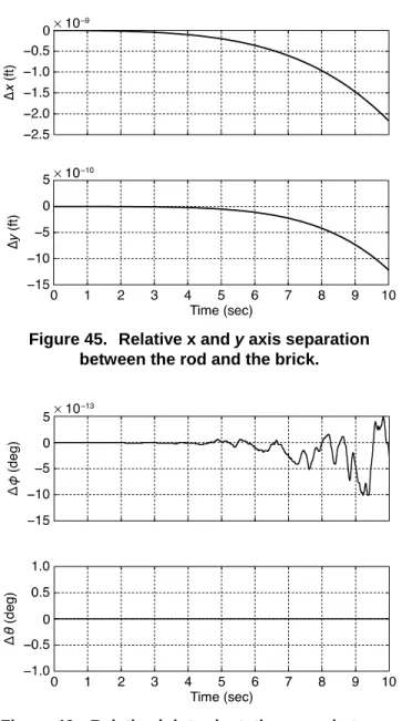
Figure 45. Relative x and y axis separation between the rod and the brick. ... 49

Figure 46. Relative joint orientation error between the joint connections of the rod and brick. ... 49

(11)

Figure 48. Inertial position comparison between ADAMS®

and POST2/CFE for the universal joint. ... 51 Figure 49. Inertial velocity comparison between ADAMS®

and POST2/CFE for the universal joint. ... 52 Figure 50. Euler angle (1-3-2 sequence) comparison between

ADAMS®_{and POST2/CFE for the universal joint. ... 53}

Figure 51. Body axis angular velocity comparison between

Figure 52. Constraint force (at the joint) comparison between

Figure 53. Constraint torque (at the joint) comparison between

Figure 54. Relative joint separation between the connection

points of Box 1 and 2 for universal joint... 56 Figure 55. Relative joint orientation error between the joint

connections of Box 1 and 2 for universal joint. ... 56 Figure 56. Test Case 7: Planar joint test case. ... 57 Figure 57. Cylinder inertial position comparison between

ADAMS®_{and POST2/CFE for the planar joint. ... 58}

Figure 58. Cylinder inertial velocity comparison between

Figure 59. Euler angle (1-3-2 sequence) comparison between

Figure 60. Cylinder body axis angular velocity comparison between

Figure 61. Constraint force (at the joint) comparison between

Figure 62. Constraint torque (at the joint) comparison between

Figure 63. Relative joint separation between the cylinder and table

connection points, represented in inertial frame components. ... 61 Figure 64. Relative joint orientation error between the joint

connections of the table and cylinder. ... 62 Figure 65. Box 1 inertial position comparison between POST2/CFE

standard spherical joint and generalized joint. ... 63 Figure 66. Box 1 inertial velocity comparison between POST2/CFE

standard spherical joint and generalized joint. ... 64 Figure 67. Box 1 Euler angle (1-3-2 sequence) comparison between

POST2/CFE standard spherical joint and generalized joint. ... 65 Figure 68. Box 1 body axis angular velocity comparison between

(12)

Figure 69. Constraint force comparison between POST2/CFE

standard spherical joint and generalized joint. ... 67

Figure 70. Constraint torque comparison between POST2/CFE standard spherical joint and generalized joint. ... 68

Figure 71. Relative joint separation between the connection points of Box 1 and 2, represented in the body frame of Box 1. Universal Joint. ... 69

Figure 72. Box 1 inertial position comparison between POST2/CFE standard universal joint and generalized joint. ... 70

Figure 73. Box 1 inertial velocity comparison between POST2/CFE standard universal joint and generalized joint ... 71

Figure 74. Box 1 Euler angle (1-3-2 sequence) comparison between POST2/CFE standard universal joint and generalized joint. ... 72

Figure 75. Box 1 body axis angular velocity comparison between POST2/CFE standard universal joint and generalized joint. ... 73

Figure 76. Constraint force comparison between POST2/CFE standard universal joint and generalized joint ... 74

Figure 77. Constraint torque comparison between POST2/CFE standard universal joint and generalized joint. ... 75

Figure 78. Relative joint separation between the connection points of Box 1 and 2. ... 76

Figure 79. Relative joint orientation error between the joint connections of Box 1 and 2. ... 76

Figure 80. Cylinder inertial position comparison between POST2/CFE standard planar joint and generalized joint. ... 77

Figure 81. Cylinder inertial velocity comparison between POST2/CFE standard planar joint and generalized joint. ... 78

Figure 82.

Cylinder Euler angle (1-3-2 sequence) comparison between POST2/CFE standard planar joint and generalized joint. ... 79

Figure 83. Cylinder body axis angular velocity comparison between POST2/CFE standard planar joint and generalized joint. ... 80

Figure 84. Constraint force comparison between POST2/CFE standard planar joint and generalized joint. ... 81

Figure 85. Constraint torque comparison between POST2/CFE standard planar joint and generalized joint. ... 82

Figure 86. Relative joint separation between the cylinder and table connection points, represented in inertial frame components. ... 83

Figure 87. Relative joint orientation error between the joint connections of the table and cylinder. ... 83

Figure 88. Space Shuttle vehicle configuration. ... 84

Figure 89. Schematic illustration of Space Shuttle staging events. ... 85

Figure 90. Attachment of SRBs to OET. ... 86

(13)

Figure 92. Variation of relative distances Δx, Δy and Δz

with time during SRB separation, STS-1. ... 88

Figure 93. Variation of OET linear acceleration components (excluding gravity) during separation. ... 89

Figure 94. Variation of LSRB linear acceleration components (excluding gravity) during separation. ... 90

Figure 95. Variation of RSRB linear acceleration (excluding gravity) components during separation. ... 91

Figure 96. Variation OET of angular velocity components during separation, STS-1. ... 92

Figure 97. LSRB: Angular velocity components during separation, STS-1. ... 93

Figure 98. RSRB: Angular velocity components during separation, STS-1. ... 94

Figure 99. Artistic rendering of X-43A (RV) separation from HXLV booster. ... 95

Figure 100. Dimensioned drawing of mated X-43A Research Vehicle and Hyper-X Launch Vehicle. ... 95

Figure 101. CFE modeling of piston contact for X-43A separation problem. ... 95

Figure 102. Comparison of joint displacement in x, y, and z directions for CFE and spring model. ... 97

Figure 103. Comparison of relative angular displacement between POST2/CFE and spring model. ... 97

Figure 104. Comparison of constraint forces computed by POST2/CFE and spring model. ... 98

Figure 105. Comparison of constraint (torques) computed by POST2/CFE and spring model. ... 98

Figure 106. Simulation versus flight data comparison of angle of attack and angle of sideslip profiles. ... 99

Figure 107. Simulation versus flight data comparison of x, y, and z accelerations in the local body frame. ... 100

Figure 108. Hyper-X simulation versus flight data comparison of body roll, pitch, and yaw rate profiles. ... 100

Figure 109. Schematic of the bimese booster and orbiter configuration. ... 101

Figure 110. Booster and orbiter dimensions and attachments (dimensions in feet). ... 102

Figure 111. Flight profile for the bimese configuration. ... 102

Figure 112. Velocity profile for the complete mission. ... 103

Figure 113. Altitude profile for the complete mission. ... 103

Figure 114. Relative separation distances between orbiter and booster. ... 109

Figure 115. Angle-of-attack variation during separation. ... 109

Figure 116. Comparison of separation distances between orbiter and booster. ... 109

Figure 117. Comparison of booster and orbiter angles of attack during separation. ... 109

(14)

(15)

Nomenclature

A*, B* mass centers of body A and body B

ax , ay , az sensed acceleration components along body axes (excludes gravity) in Space

Shuttle SRB separation problem, ft/sec2 a

^ _{acceleration vectors with components a}

x , ay , az

a

^

1, a^2, a^3 unit vectors fixed in body A b

^

1, b^2, b^3 unit vectors fixed in body B

, generic unit vectors fixed in body A and in body B f generalized force matrix

(CON) _{joint constraint force vector with components F}

x , Fy , Fz

(EXT)_, (EXT) _{external force vectors acting on body}_A_{and body}_B,_{Euclidean vectors}_,

independent of reference frame

g Baumgarte constraint function

I A ,IB inertia dyadic of body A and body B

Ixx , Iyy , Izz moment of inertia about body x, y, and z axes, slugs ft2

lref vehicle reference length, ft

M generalized mass matrix as defined in Eq. (29) and Eq. (71)

m A , mB mass of body A and body B, slugs n

^

1, n^2, n^3 unit vectors fixed in inertial reference frame

p, q, r angular velocity components along x, y and z body axes, deg/s

qi generalized coordinates, i = 1, 2,….

∗

inertial position vector of mass center of body A, ft

∗

inertial position vector of mass center of body B, ft

̅ ̿ _{position vector from ̅ to ̿, ft}

(CON) _{joint constraint torque vector with components}

Tx , Ty , Tz

generalized motion variable matrix with elements , i = 1, 2, 3….

v mass center velocity vector, with components

v

x

, v

y

, v

z

Δx, Δy, Δz joint displacements in x, y, z direction, also separation distance between OET and SRBs in x, y, z directions, ft

α angular acceleration vector, rad/sec2

α matrix defined in Eq. (30)

φ, _θ, _ψ Euler angles in roll, pitch and yaw, deg

Δφ, _Δθ, _Δψ joint rotational constraint errors, deg

γ matrix defined in Eq. (31)

(16)

ω angular velocity vectors relative to an inertial reference frame with components ωx , ωy , ωz,, rad/sec

η Baumgarte parameter

Suffixes

A, B body A, body B

b body axes system

Acronyms

Abs Max Diff absolute maximum difference

CFE constraint force equation CG center of gravity

ConSep Conceptual Separation DOF degrees of freedom

ET external tank

HXLV Hyper-X launch vehicle

IRVE Inflatable Reentry Vehicle Experiment LGBB Langley Glide Back Booster

LSRB left solid rocket booster

NASA National Aeronautics and Space Administration NGLT next generation launch technology

OET Orbiter and external tank

POST2 Program to Optimize Simulated Trajectories II RKF45 Runge-Kutta-Fehlberg 45 (MATLAB®_function)

RSRB right solid rocket booster RV research vehicle

SRB solid rocket booster SSME Space Shuttle main engine SSTO single-stage-to-orbit

STS space transportation system SVDS Shuttle vehicle dynamic simulation TSTO two-stage-to-orbit

(17)

Section 1. Introduction

The problems with the dynamic separation of multiple bodies within the atmosphere are complex and challenging. A few problems that have received significant attention in the literature are the store separation from aircraft (ref. 1), and the separation of the X-15 research vehicle from the B-52 carrier aircraft (ref. 2). For both of these cases, the store and the X-15 vehicle are much smaller in size than the parent vehicle. The other class of stage separation problem involves the separation of two vehicles of comparable sizes as in the case of multi-stage reusable launch vehicles where the integrity of each stage is important after separation. Reference 3 presents a method for computing six degrees of freedom (DOF) trajectories of hinged/linked vehicles. Reference 4 reports a summary of stage separation capabilities in the 1960s and 1970s.

NASA studies on stage separation of multistage reusable launch vehicles date back to the 1960s (refs. 5–9). More recently, Naftel et al. (refs. 10–12) considered the staging of two wing-body vehicles. NASA’s Next Generation Launch Technology (NGLT) Program identified stage separation as one of the critical technologies needed for the successful development and operation of next generation multistage reusable launch vehicles (ref. 13). In response to this directive, the stage separation analysis and simulation tool called Conceptual Separation (ConSep) was developed (ref. 14). ConSep is a MATLAB®_{based front end to the ADAMS}®_{solver, which is an industry standard}

commercial software for solving dynamics problems involving multiple bodies connected by joints. References 14 and 15 discuss applications of ConSep for two-body (two-stage-to-orbit, TSTO) and three-body (Space Shuttle solid rocket booster, SRB) separations. However, for performing seam-less end-to-end simulations of complete launch vehicle trajectories including stage separation, as recommended by the X-43A (Hyper-X) Return-To-Flight Review Board (ref. 16), ADAMS® _{has to be}

linked to a trajectory simulation code like the Program to Optimize Simulated Trajectories II (POST2) because POST2 cannot model internal forces and moments at the joints. However, linking ADAMS®_{(ref. 17) with POST2 for end-to-end simulations is user-intensive and requires elaborate}

pre and post processing to run ConSep as an interface to ADAMS®_{. Moreover, linking codes is not}

generic and typically involves extensive customization for analysis of each stage separation prob-lem. Instead, it would be preferable to have a built-in generic multi-body dynamics simulation capability, including stage separation, as an integral part of trajectory simulation and optimization software like POST2. The availability of such a capability greatly facilitates end-to-end simulation of launch vehicle trajectories and eliminates any chance for possible hand-off errors.

This report discusses application of the constraint force equation (CFE) method for calculating internal constraint forces and constraint moments associated with ideal joints that connect multiple rigid bodies belonging to a flight vehicle. Constraint forces and constraint moments are applied as though they were external forces and moments. The calculations are based on a well-known approach involving Lagrange multipliers, sometimes referred to as undetermined multipliers (refs. 18-20), where the scalar multipliers have very clear relationships to the force and moment vectors as established in ref. 21. Thus, with application of the CFE methodology, the problem of the motion of multiple bodies connected by joints is reduced to one of multiple free body motions subject to the applied external forces and moments and the additional constraint forces and moments computed by CFE. When the joints connecting the vehicles are released, these additional forces and moments vanish, and the vehicles are in free motion. Basically, CFE methodology properly simulates the motion of these bodies in close proximity and assigns proper initial conditions for the free, unconstrained motion of multiple vehicles following joint release. To demonstrate the CFE methodology, several individual test cases were developed featuring various

(18)

types of simple joints. To validate CFE methodology, the test case results were compared with those predicted using the ADAMS®_{solver, except for fixed joint case, where the CFE results were}

compared with those predicted using AUTOLEV (ref. 22), which is another industry standard software. Having tested and validated each of these cases individually, the concept of a generalized joint was developed that greatly facilitates the use of CFE because the user can simply assign proper DOFs to joints connecting multiple bodies without needing to know the details of CFE methodology.

The CFE methodology discussed in this report is generic and can be implemented and inte-grated in any trajectory optimization software. This report discusses the implementation of CFE in POST2 (ref. 23), an industry-standard trajectory simulation and optimization software package de-veloped in the early 1970s. Since then, POST2 has been under continuous development and im-provement. POST2 can be used to simulate three and six DOF motion for multiple, unconnected free-flying vehicles. For the simulation of launch vehicle staging, it is necessary to model two or more vehicles connected by simple joints, the release of those joints, and the subsequent free flight motion of each body. The current version of POST2 does not have the capability to model internal joint forces and moments prior to separation when the separating bodies are still connected. With CFE implementation, POST2 will have the capability for seamless and efficient end-to-end simula-tion of launch vehicle trajectories including stage separasimula-tion. This approach allows the user to use all modeling and optimization features of POST2.

The POST2/CFE methodology has been applied to launch vehicle stage separation problems. Three cases are discussed: (i) the Space Shuttle SRB separation from the Orbiter and external tank (OET), (ii) the Hyper-X research vehicle separation from the Pegasus booster, and, (iii) the end-to-end simulation of a conceptual TSTO Bimese vehicle. For the first two cases, the POST2/CFE predic-tions are compared with available flight test data. The objective of the third case is to demonstrate the convenience of POST2/CFE for the seamless end-to-end simulation of launch vehicle trajecto-ries including stage separation.

It should be noted that even though emphasis in this report is on the application of CFE meth-odology to multi-body separation problems, it is not necessary that the bodies become separated during the simulation. The basic CFE methodology is applicable to multiple bodies that stay con-nected throughout the simulation. Such an application of the CFE algorithm to the IRVE (Inflatable Reentry Vehicle Experiment) vehicle is discussed in ref. 24.

(19)

Section 2. Constraint Force Equation Methodology and

Implementation in POST2

The basic concept of CFE methodology can be illustrated with the help of an example involving the motion of two rigid bodies and connected by a single revolute joint, as shown in Fig. 1(a). The set of external forces acting on is equivalent to a force ( ) applied at ∗_{, the mass center}

of , together with a couple whose torque is ( ); this set typically includes gravitational, aerodynamic, and propulsive forces. Similarly, the set of external forces acting on is equivalent to a force ( ) applied at ∗_{, the mass center of , together with a couple whose torque is} ( )_.

The constraints imposed by the joint are satisfied when a set of internal forces is applied by body to body . The set is equivalent to a single constraint force ( )_{applied at a single point of}

con-tact, together with a couple whose torque is ( )_{, as shown in Fig. 1(b). According to the law of}

action and reaction, a force of equal magnitude and opposite direction, − ( )_{, is applied by to}

, along with a couple whose torque is − ( )_{. The objective of the CFE algorithm is to compute} ( )_and ( )_{; they depend on the type of joint and the external forces acting on and .}

Figure 1(c) illustrates the way in which the CFE algorithm can be implemented in trajectory simula-tion software like POST2. At each integrasimula-tion time step, POST2 computes all the external forces and moments acting on each vehicle. This information, along with specific geometric information about the joint, is passed to the CFE algorithm, which works in parallel with POST2. The CFE algorithm computes the internal constraint forces and moments and passes the data back to POST2, which applies them as additional external forces and moments on each body. Thus, the net external forces and moments on each vehicle are the sum of the usual external forces and moments and the joint loads applied to each vehicle as additional external forces and moments. Then, POST2 computes the rotational and translational accelerations of each body, and the solution is propagated in the usual manner with POST2 communicating to CFE at each time step. Consequently, the CFE joint model simply augments the vehicle’s external loads and does not require major modification to the equations of motion built in POST2. If the joint connecting the two bodies is released, the constraint forces and moments vanish, and the two bodies move independently of each other.

Two approaches to the CFE method are presented in what follows. The first approach, dis-cussed in Sec. 2.1, is a variation of what the authors reported in Refs. 25 and 26. (Some of the no-menclature and notation in this report differs from what is in Refs. 25 and 26.) In general, it in-volves a number of unnecessary equations used to indicate an absence of constraint forces and/or constraint torques in certain directions. In contrast, there are no more equations than absolutely necessary in the second approach; it is presented in Sec. 2.2, and is known as the conventional Lagrange multiplier method. In this study, we employ the more computationally efficient Lagrange multiplier method.

(20)

(a) External forces and moments. (b) Internal forces and moments.

(c) Revolute joint implementation. (d) Translational joint implementation. Figure 1. Schematic Illustration of CFE methodology.

(21)

2.1 Method

I

When two rigid bodies and are connected by a single revolute joint as shown in Fig. 1(c), dynamical equations governing constrained motion in an inertial reference frame can be expressed in terms of vectors (denoted by boldface symbols) as follows. For body ,

( )₋ ₍ ₎₌ ₍₁₎

( )₋ ∗ _̅

× ( )₋ ( )₌ _∙ ₊ _× _⋅ ₍₂₎

where is the mass of , is the angular velocity of in an inertial reference frame, is the angular acceleration of in an inertial reference frame, is the acceleration in an inertial reference frame of ∗_{, the mass center of , and where is the inertia dyadic of with respect}

to ∗_{. The position vector from} ∗_{to ̅, the joint location of body , is denoted by} ∗ _̅

. Like-wise, the corresponding equations for body are

( )₊ ₍ ₎ ₌ ₍₃₎

( )₊ ∗

× ( )₊ ( )₌ _⋅ ₊ _× _⋅ ₍₄₎

where ∗ represents the position vector from ∗_{, the mass center of , to , the joint location}

of .

Suppose that the revolute joint is replaced by a joint that permits relative translation between body and body as shown in Fig. 1(d). In that case the contact point fixed in does not in general remain coincident with ̅, and ̿ denotes the point of that is instantaneously coinci-dent with . Because the constraint force − ( )_{is presumed to be applied to at ̿, the}

mo-ment of this constraint force about ∗_{is simply} ∗ ̿_{× [−} ( )_{], and Eq. (2) is replaced with}

( )₋ ∗ _̿

× ( )₋ ( )₌ _⋅ ₊ _× _⋅ ₍₅₎

In the case of unconstrained motion, ( )_and ( )_{are identically zero and Eqs. (1), (3),}

(4), and either (2) or (5) reduce to standard dynamical equations of motion for two independent rigid bodies, yielding a total of 12 scalar equations for 12 unknown quantities, namely, three scalars associated with each of the accelerations, and , and the angular accelerations, and . The present method is based on the assumption that during constrained motion there are three additional unknown scalar quantities associated with each of ( ) and ( )_{. (In fact, it is}

well established in the literature that the required number of additional unknowns is equal to the number of independent constraint equations that characterize a joint, and that this number is always less than six.) Hence, we are in search of six additional scalar equations, and they are obtained by considering the joint constraints in the following way. First, form linearly independent constraint equations that describe restrictions imposed by the joint on relative translation and/or relative rotation. Second, consider the translation or rotation that is permitted by the joint, assume the joint is ideal (with perfectly smooth, frictionless bearing surfaces), and write equations that state certain components of ( ) and/or ( )_{are zero.}

(22)

When a joint constrains relative translation, the distance in a particular direction between ̅ and must remain zero; that is,

( − ̅) ⋅ = 0 (6)

where is the position vector to from a point fixed in an inertial reference frame, ̅ is the position vector from to ̅, and where is taken to be a unit vector fixed in in a direction for which translational motion is prohibited by the joint. One relationship having the form of Eq. (6) is needed to account for each direction in which translation is constrained. For example, a fixed joint constrains translation in three orthogonal directions; therefore, three relationships hav-ing the form of Eq. (6) are required. In each such equation, the role of is played by one of three mutually orthogonal unit vectors fixed in . For a prismatic (sliding) joint that permits translation in only one direction (and restricts translation in two perpendicular directions), two expressions having the form of Eq. (6) are required.

A constraint on relative rotation can be viewed as a requirement that two unit vectors, and , must remain perpendicular to each other throughout the constrained motion; is fixed in body , and is fixed in body , such that they are each perpendicular to the axis about which rotation would take place if the constraint were not present. The constraint is expressed by setting the scalar product of the two unit vectors equal to zero,

⋅ = 0 (7)

One relationship having the form of Eq. (7) is required for each direction about which rotation is constrained; no more than three such relationships are associated with any one joint.

Equations (6) and (7) must be differentiated twice with respect to time so that the resulting constraint equations involve the unknown mass center accelerations and , and angular ac-celerations and , that appear in Eqs. (1), (3), (4), and either (2) or (5). Thus, the second derivatives requiring development are

− ̅ ⋅ = 0 (8)

( ⋅ = 0) (9)

It is convenient to form the required derivatives by differentiating each vector with respect to time in an inertial reference frame.

Now, the position vector ̅ can be written as ∗+ ∗ ̅, where ∗ ̅ is a vector fixed in . The time derivative in an inertial reference frame of ∗ is , the velocity of ∗_{in an inertial}

reference frame. The time derivatives in an inertial reference frame of ∗ ̅ and are ×

∗ _̅

and × , respectively. The time derivatives of and can be treated similarly. Hence, the result of differentiating Eq. (6) once is

(23)

The second differentiation yields

+ × ∗ + × × ∗ − − × ∗ ̅− × × ∗ ̅ ⋅

+ 2 + × ∗ − − × ∗ ̅ ⋅ ( × )

+ − ̅ ⋅ ( × + × × ) = 0 (11)

An alternative form of Eq. (11) will prove useful in Sec. 2.3. It is obtained by making use of re-lationships involving position vectors,

− ̅ = (12)

∗ _̅

+ = ∗ (13)

and identities for scalar triple products,

⋅ × = × ⋅ = − × ⋅ = − ⋅ × (14) to write − ̅ ⋅ ( × ) = ⋅ ( × ) = − × ⋅ (15) and − × ∗ ̅ ⋅ + − ̅ ⋅ ( × ) = − × ∗ ̅ ⋅ − × ⋅ = − × ∗ ̅+ ⋅ = − × ∗ ⋅ (16)

Hence, Eq. (11) can also be expressed as

+ × ∗ + × × ∗ − − × ∗ − × × ∗ ̅ ⋅

+ 2 + × ∗ − − × ∗ ̅ ⋅ ( × )

+ ̅ ⋅ ( × × ) = 0 (17) As for the rotational constraint, differentiating the terms in Eq. (7) once with respect to time yields

( × ) ⋅ + ⋅ ( × ) = 0 (18)

In view of identities for scalar triple products, the two terms in the left-hand member can be written as

( × ) ⋅ = ⋅ × (19)

(24)

⋅ ( × ) = − ⋅ × (20) Hence, Eq. (18) can be restated as

( − ) ⋅ ( × ) = 0 (21)

Differentiating once more gives

( − ) ⋅ ( × ) + ( − ) ⋅ [( × ) × + × ( × )] = 0 (22) When relative translation is permitted in a certain direction, an equation having the form of Eq. (11) is not applicable in that direction. Likewise, when relative rotation is allowed, a relationship having the form of Eq. (22) is not applicable. Instead, the required equations can be obtained using the condition that the constraint force or torque is zero in those directions (with the assumption that the surfaces of the joint are perfectly smooth) in which free translation or rotation is permit-ted. Thus, for a joint that permits translation in a certain direction parallel to the vector ,

( )_{⋅ = 0} ₍₂₃₎

Similarly, when a joint permits relative rotation about an axis parallel to the vector ,

( )_{⋅ = 0} ₍₂₄₎

As may be noted in Sec. 2.2, the Lagrange multiplier method does not require the use of equations having the form of (23) and (24).

In summary, equations having the form of (11) and (22)–(24) provide, in combination, a total of six remaining equations.

The 18 scalar equations formed from Eqs. (1), (3), (4), (11), (22)–(24), and either (2) or (5), are linear in 18 unknowns. Three variables represent each of the two mass center accelerations, each of the two rigid body angular accelerations, the constraint force, and the constraint torque, for a total of 18 unknowns. These equations can be expressed in matrix form as = (where the column matrix contains the 18 unknown parameters) and solved using standard matrix inversion techniques. A variation of this formulation was presented in Refs. 25 and 26 and applied to the case of two bodies connected by a fixed joint, as well as the problem of separation of the Hyper-X vehicle from the Pegasus booster. Both of these cases are included in this report and discussed in Secs. 3.1.1 and 4.2, respectively.

2.2 Method II: Lagrange Multiplier Method

As mentioned in connection with Eqs. (1)–(5), dynamical equations governing the uncon-strained motion of bodies and can be expressed in vector form as

( )₌ ₍₂₅₎

(25)

( )₌ ₍₂₇₎

( )₌ _⋅ ₊ _× _⋅ ₍₂₈₎

In general, the collection of dynamical differential equations governing unconstrained motion of , , and other rigid bodies can be written in matrix form as

= (29)

where is a square generalized mass matrix, is a column matrix containing generalized accelerations, and is a column matrix containing generalized forces, nonlinear terms arising from gyroscopic torque, etc. The object of the CFE method is to modify Eqs. (29) such that they become applicable when rigid bodies are connected by joints. The modification is carried out using a well-known approach involving Lagrange multipliers, sometimes referred to as undetermined multipliers,

= + (30)

where is a column matrix containing the multipliers. Linearly independent equations describing the constraints imposed by the joints are written in matrix form as

+ = 0 (31)

where is a column matrix, and the right-hand member is a column matrix whose elements are all zero. The matrix appearing in Eqs. (30) is the transpose of the coefficient matrix in Eqs. (31). (Bold font and a subscript are used to distinguish angular acceleration, for example, from the coefficient matrix .) The product is a column matrix containing generalized constraint forces. Equations (30) can be solved for ,

= ( + ) (32)

and substitution from Eqs. (32) into (31) yields

( + ) + = 0 (33)

or

= −( + )

Hence,

= −( ) ( + ) (34)

The number of multipliers in the matrix λ is exactly equal to the number of constraint equations (31).

(26)

2.3 Constraint Equations in Matrix Form

Constraint equations given in vector form in Sec. 2.1 can be rewritten in matrix form as stated in Eqs. (31). Examples are now given using the acceleration-level relationships for a translational constraint, Eq. (11), and a rotational constraint, Eq. (22). A system of two bodies performing uncon-strained motion in an inertial reference frame possesses 12 degrees of freedom; thus, for two constraints, is a 2 × 12 matrix, is a 12 × 1 column matrix, and is a 2 × 1 column matrix.

Let n^

r (r = 1,2,3) be a set of right-handed, mutually orthogonal unit vectors fixed in an inertial

reference frame, and let unit vectors a^_r_and_b^

r (r = 1,2,3) be two similar sets fixed in and in ,

respectively. The velocity of the mass center of in an inertial reference frame can be written in terms of n^

1, n^2, and n^3,

= + + (35)

The angular velocity of in an inertial reference frame can be expressed in terms of a^

1, a^2,

and a^

3 ,

= + + (36)

The acceleration of the mass center of in an inertial reference frame is then given by

= + + (37)

The angular acceleration of in an inertial reference frame is

= + × = + = + + (38)

where ( / ) represents differentiation with respect to time in reference frame . Correspond-ing quantities associated with are written similarly,

= + + = + + (39)

= + + = + + (40)

A constraint on translation is chosen as the first constraint in the present example. Upon substitution from Eqs. (35)–(40) into (17), one can inspect the result to identify the coefficient _, of for = 1, … ,12 to form the first row of the matrix .

, = − ⋅ , = − ⋅ , = − ⋅ (41) , = − × ∗ ⋅ , = − × ∗ ⋅ , = − × ∗ ⋅ (42) , = ⋅ , = ⋅ , = ⋅ (43) , = × ∗ ⋅ _, = × ∗ ⋅ _, = × ∗ ⋅ (44)

(27)

The first element of the matrix consists of all terms in Eq. (17) that do not involve , … , .

= × × ∗ − × × ∗ ̅ ⋅

+ 2 + × ∗ − − × ∗ ̅ ⋅ ( × )

+ ⋅ ( × × ) (45) In the current example a constraint on rotation is chosen as the second constraint, and substitution from Eqs. (35)–(40) into (22) yields a result that is inspected to identify the coefficient _, of for = 1, … ,12 to form the second row of the matrix .

, = 0 , = 0 , = 0 (46)

, = − ⋅ × , = − ⋅ × , = − ⋅ × (47)

, = 0 , = 0 , = 0 (48)

, = ⋅ × , = ⋅ × , = ⋅ × (49)

The second element of the matrix consists of all terms in Eq. (22) that do not involve , … , .

= ( − ) ⋅ [( × ) × + × ( × )] (50)

2.4 Baumgarte Constraint Stabilization Method

The matrices , , , and are used together with Eqs. (34) to determine values of the mul-tipliers needed to enforce the constraints at any instant of time. With the column matrix con-taining the generalized constraint forces in hand, constrained motion can be simulated by perform-ing numerical integration of Eqs. (30) and an appropriate set of kinematical differential equations. However, the numerical solution is sensitive to computational errors and initial joint misalignment errors. The accumulation of the numerical errors may lead to a significant joint displacement or misalignment over time, an artifact referred to as constraint drift. In order to control constraint drift, the CFE algorithm employs a technique known as Baumgarte stabilization (Ref. 27), which is applicable to methods I and II.

The constraint equations (31) can be expressed as

+ = = 0 (51)

where 0 is a column matrix whose elements are all zero, and where is a column matrix contain-ing the left-hand members of (non-differentiated) configuration constraint relationships obtained from Eqs. (6) and (7). The stabilization technique is implemented by augmenting Eqs. (51) with terms involving the once-differentiated and non-differentiated forms of :

(28)

Thus, the new constraint relations in Eqs. (52) make use of all three forms of the constraint equa-tions to produce behavior of damped, second-order systems with a damping ratio of 1. The stiff-ness, which determines frequency, is represented by , a scalar constant whose value is selected by the analyst to control the constraint drift. Reference 27 suggests values of ranging from 0 to 10. Substitution from Eqs. (51) into (52) yields

+ + 2 + = 0 (53)

In other words, the Baumgarte method consists of replacing Eqs. (31) with relationships expressed as

+ = 0 (54)

where

= + 2 + (55)

As in Sec. 2.3, a translational constraint and a rotational constraint can be used as examples to demonstrate how to form 2 × 1 column matrices , , and . In the case of a translational con-straint, refer to Eq. (6) to write the position-level constraint as

( ) = − ̅ ⋅ = 0 (56)

Refer to Eq. (10) to express the corresponding velocity-level constraint as

( ) = + × ∗ − − × ∗ ̅ ⋅ + − ̅ ∙ ( × ) = 0(57)

Finally, the acceleration-level constraint is obtained from Eq. (11),

( ) = + × ∗ + × × ∗ − − × ∗ ̅− × × ∗ ̅ ⋅

+ 2 + × ∗ − − × ∗ ̅ ⋅ ( × )

+ − ̅ ⋅ ( × + × × ) = 0 (58) Similarly, the rotational constraint at the position, velocity, and acceleration levels are obtained from Eqs. (7), (21), and (22), respectively.

( ) = ⋅ = 0 (59)

( ) = ( − ) ⋅ ( × ) = 0 (60)

(29)

2.5 Planar Motion of Two Bodies Constrained by Slider Joint

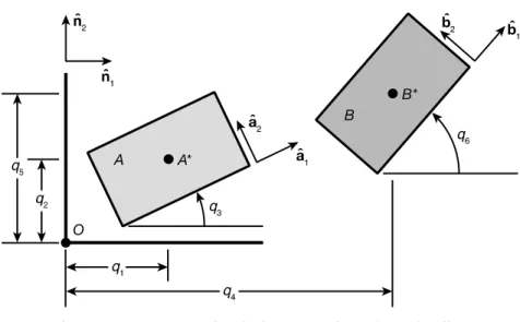
Use of the relationships presented in the preceding sections is illustrated with an example involving planar motion of two rigid bodies connected by a slider joint. Let n (r = 1,2,3) be a set of right-handed, mutually orthogonal unit vectors fixed in an inertial reference frame such that n and n lie in the plane of motion, as shown in Fig. 2, and n is perpendicular to the plane. Let unit vectors a and b (r = 1,2,3) be two similar sets fixed in A and in B, respectively, with a and b each parallel to a central principal axis of inertia of the body in which it is fixed.

Motion of is regarded as unconstrained when the mass center ∗_{can translate in the plane,}

and the body can rotate about an axis parallel to . Likewise, is unconstrained when it can move completely independently of . Thus, the unconstrained system possesses six degrees of freedom in an inertial reference frame, and six generalized coordinates , … , are required to specify the configuration of the system. These coordinates are defined operationally by writing

∗

≜ + ⋅ ≜ cos (62)

∗

≜ + ⋅ ≜ cos (63)

where, ∗ and ∗ denote the position vectors to ∗_and ∗_{, respectively, from a point fixed}

in an inertial reference frame. Translational coordinates , , , and are indicated in Fig. 2, as are angles and . It will prove useful in what follows to refer to direction cosine matrices that indicate how unit vectors and , respectively, are related to ( = 1,2,3).

Figure 2. Unconstrained planar motion of two bodies A and B in inertial reference system.

Six motion variables , … , can be defined with the kinematical differential equations

(30)

and subsequently used to write

= + = = (65)

= + = = (66)

= + = = (67)

= + = = (68)

The external forces ( ) and ( ), as well as the external torques ( ) and ( ), can be expressed as

( ) ₌ ₊ ( )₌ ₌ ₍₆₉₎

( ) ₌ ₊ ( ) ₌ ₌ ₍₇₀₎

This brings one into position to use Eqs. (25) and (26) for , together with Eqs. (27) and (28) for , to identify the matrices , , and appearing in Eqs. (29),

= 0 0 0 0 0 0 0 0 0 0 0 0 0 0 0 0 0 0 0 0 0 0 0 0 0 0 0 0 0 0 = = (71)

and then to express the dynamical equations of unconstrained motion represented by Eqs. (29), as

0 0 0 0 0 0 0 0 0 0 0 0 0 0 0 0 0 0 0 0 0 0 0 0 0 0 0 0 0 0 = (72)

where is the central principal moment of inertia of for an axis parallel to , and is the central principal moment of inertia of for an axis parallel to .

We now regard body as attached to body with a slider joint that permits relative transla-tion in the directransla-tion of , but prevents relative translation in the direction of , and prohibits relative rotation about = . In this case, the constrained system possesses four degrees of freedom in an inertial reference frame. Points ̅ and are chosen as material points of and , respectively, that lie on the axis of the sliding joint as shown in Fig. 3. In the interest of simplicity they are chosen such that

∗ _̅

(31)

where and are positive constants. It is worth keeping in mind that ∗ = ∗ ̿ because ̿ is the point of that is instantaneously coincident with .

Figure 3. Constrained planar motion of bodies A and B in inertial reference system.

A translational constraint equation is obtained by letting play the role of in Eq. (6).

= ( ) = − ̅ ∙ a = 0 (74)

The position vectors from to ̅ and to can be expressed as

̅₌ ∗

+ ∗ ̅ = + + (75)

= ∗+ ∗ = + − (76)

Hence, Eq. (74) can be restated as

= ( − )( ∙ ) + ( − )( ∙ ) − − ∙ = 0 (77)

Table 1. Direction Cosine Matrices.

cos q3 –sin q3 0 cos q6 –sin q6 0

sin q3 cos q3 0 sin q6 cos q6 0

0 0 1 0 0 1

After referring to Table 1 to obtain the dot products

(32)

one can write

= − ( − )sin + ( − ) cos − − cos( − ) = 0 (79) The derivatives and can be obtained either by differentiating Eq. (79) successively with respect to time, or by appealing to Eqs. (57) and (58), respectively. In either case, one obtains

= [ − − ( − ) ] cos − [ − + ( − ) ] sin + ( − ) sin ( − ) = 0 (80) and = [ − − 2( − ) − ( − ) − ( − ) ] cos − [ − + 2( − ) + ( − ) − ( − ) ] sin + [( − ) sin ( − ) + ( − ) cos ( − )] = 0 (81)

A rotational constraint equation is obtained from Eq. (7) by letting and play the parts of and , respectively.

= ( ) = ⋅ = sin ( − ) = 0 (82)

The derivatives and can be obtained by employing Eqs. (60) and (61) respectively. How-ever, a significant amount of labor can be saved by simply differentiating Eq. (82) successively with respect to time to produce

= ( − ) cos ( − ) = 0 (83)

and

= ( − ) cos ( − ) − ( − ) sin ( − ) = 0 (84)

The reason for retaining sin(q3-q6) in Eq. (84) is that, due to constraint drift, Eq. (82) may not be

satisfied identically. The error in sin (q3 - q6) is controlled by the Baumgarte method, as indicated in

Eqs. (52), (53), and (55). Inspection of Eqs. (81) and (84) for the coefficients of , … , allows one to identify the elements of the matrix α in Eqs. (54). For convenience, the transpose of α is recorded as

=

sin 0

− cos 0

−( − ) sin − ( − ) cos + sin ( − ) cos ( − )

− sin 0

cos 0

− sin ( − ) − cos ( − )

(85)

The 2 × 1 matrix in Eqs. (55) is constructed with the terms in Eqs. (81) and (84) that do not involve , … , and with Eqs. (79), (80), (82), and (83).

(33)

= −2 [( − ) cos + ( − ) sin ] + [( − ) sin − ( − ) cos ] + ( − ) cos ( − )

+ 2 [ − − ( − ) ] cos − [ − + ( − ) ] sin + ( − ) sin ( − )

+ [( − ) cos − ( − ) sin − − cos ( − )] (86)

= −( − ) sin ( − ) + 2 ( − ) cos ( − ) + sin ( − ) (87)

In this example, two independent equations (74) and (82) describe the constraint imposed by the slider joint. Hence, precisely two unknown multipliers ( ) and ( ) are all that are neces-sary to characterize the set of internal forces associated with the joint. The two multipliers in the matrix are determined at any instant of time by using Eqs. (34) and the matrices , , , and . Subsequently, the generalized constraint forces are formed as

=

sin − cos

[−( − ) sin − ( − ) cos + sin ( − )] + cos ( − ) − sin

cos

− sin ( − ) − cos ( − )

(88)

These generalized constraint forces are added to the right-hand member of Eqs. (72), as required by Eqs. (30), to form dynamical equations governing constrained motion of and . The dynam-ical equations, together with the kinematdynam-ical differential equations (64) and initial values of and , can be integrated numerically to obtain time histories of the generalized coordinates and motion variables ( = 1, … ,6). The accuracy of the numerical solution can be measured by the extent to which the translational and rotational constraints are unsatisfied; that is, by how much ( ) and ( ) differ from zero.

The rotational constraint equation (82) is satisfied when = ; as long as the constraint is satisfied, sin ( − ) can be replaced with 0, and cos ( − ) can be replaced with 1 in Eqs. (88).

As discussed in Refs: 21, 28 and 29, the constraint force ( )_{applied to at can be}

determined by inspecting Eq. (10) and is given by

( ) ₌ ₌ ₍₈₉₎

Similarly, the constraint torque T( )_{applied to B is identified by inspecting Eq. (21),}

( )₌ ₍ _{× ) =} ₍ _{× ) = −} ₍₉₀₎

(34)

Section 3. Test Cases

3.1 CFE Test Cases

A series of test cases was selected to validate the CFE methodology as listed in table 2. These cases include simulation models involving two rigid bodies connected by various types of simple joints. For test case 1, the geometrical shape of the two rigid bodies is defined as discussed below. However, for test cases 2–6, the geometrical shape is arbitrary and only schematic representations are shown for convenience. It is possible that depending on the geometrical shape selected for the two bodies having the same mass properties and subject to the same external force/moment as selected here, the two bodies may collide during the selected duration of simulation. Since the focus of this report is on the estimation of joint constraint loads and how they compare with ADAMS® _for

test/validation of CFE methodology, collision between two bodies, if any, are ignored.

Table 2. CFE Test Cases.

Case # Name of the Joint Description

1 Fixed Two boxes fixed to each other

2 Spherical Two boxes connected by a spherical joint

3 Revolute Two boxes connected by a revolute joint

4 Translational A box sliding along a fixed rail that is rectangular in cross section

5 Cylindrical A box sliding along a fixed rod that is circular in cross section

6 Universal Two boxes connected by a universal joint

7 Planar A thin disk sliding along a table top

3.1.1 Test Case 1: Fixed Joint

This test case involves two rectangular rigid bodies, denoted as bodies A and B with dimensions as shown, connected by a fixed joint (fig. 4). The fixed joint is a mathematical concept but serves as a rigorous test case for the CFE methodology because one knows that the joint displacement (linear and angular) must be insignificantly small (ideally zero) when the two bodies are rigidly connected, and there is no relative motion. The mass centers A*, B* and S* are respectively the centroids of body A, body B and the combined body (prior to release).

(35)

Table 3. Mass Properties for Test Case 1. Body A Body B m 1 slug 4/10 slug Ixx 5/12 slug-ft2 1/6 slug-ft2 Iyy 26/12 slug-ft2 1/6 slug-ft2 Izz 29/12 slug-ft2 4/15 slug-ft2

Table 3 shows the mass properties for each body. The fixed joint constrains the point ̅ fixed in A

to remain coincident with the point fixed in B. The three translational constraint equations have the form of Eq. (7) and can be written as

− ̅ ∙ = 0 (91)

where the role of eA in Eq. (7) is played in turn by , , and , members of a set of three

right-handed, mutually orthogonal unit vectors fixed in A at its mass center A* as shown in fig. 4. Let , , and be a similar set of unit vectors fixed in B at its mass center B* such that points in the same direction as (r = 1, 2, 3) when A and B are attached to each other. The fixed joint constrains unit vectors fixed in A to remain perpendicular to certain unit vectors fixed in B resulting in the following three constraint equations in the form of Eq. (8):

∙ = 0 (92)

∙ = 0 (93)

∙ = 0 (94)

Thus, all six constraint equations (91)–(94) characterize the fixed joint, which is the maximum number of constraint equations that can be specified for a joint. These constraint equations need to be differentiated twice to construct the matrix that contains the generalized constraint forces as illustrated earlier for the sliding joint.

3.1.1.1 Numerical Simulation

The bodies A and B are assumed to be rigidly connected to each other for first 10 sec and then “released” instantaneously. Throughout the duration of this simulation, all external forces or moments including gravity were assumed equal to zero. Because there are no external forces or moments, integrals involving linear and angular momentum must remain constant. Since the linear momentum of the combined body prior to separation is zero, after separation, the mass centers of

A and B must travel in straight lines with constant velocities such that the net linear momentum is zero and the system mass center remains at rest.

This problem was set up such that the inertial reference frame coincides with the combined body frame at t = 10 sec just prior to the joint release, the linear velocity of the combined body is zero, and the angular velocity components of the combined body were selected as (0, 2.0, 0.5) rad/sec or (0, 114.5454, 28.6363) deg/sec. Then, working backwards, the initial (t = 0) angular velocity, = 63.02 − 82.32 + 80.25 deg/sec in the body frame was deduced. With these

(36)

derived initial conditions, the simulation can be done as usual with forward integration in time releasing the joint at 10 sec and terminating the simulation at 20 sec.

To verify and validate POST2/CFE simulation results, a simulation was also created with AUTOLEV (ref. 22) an interactive program designed specifically for the kinematic and dynamic analysis of mechanical systems. For this test case, AUTOLEV was used to create a computer program to simulate the motions of A and B and determine the constraint forces required to hold them together for the first 10 seconds. The AUTOLEV results were generated using a variable step integrator with an absolute error limit of 1 × 10−8_{and a relative error limit of 1}_×₁₀−7_{. The}

POST2/CFE method employed a fixed step integrator with a step size of 0.0001 sec. The CFE routine also used a Baumgarte (ref. 27) constraint stabilization factor = 5.0.

Time histories for the inertial x, y, and z components of linear velocity of the mass centers of body A and B are shown for 20 sec in Figs. 5 and 6. Prior to release, even though the combined body has zero linear velocity, bodies A and B have nonzero linear velocity components because their mass centers A* and B* are offset from the combined mass center S*. However, the com-bined sum of each of the three components of linear momentum should be zero. This fact can be checked using mass properties from table 2 and velocity component data presented in fig. 5 and 6. The magnitudes of each of the three linear velocity components for body A and B oscillate during the first 10 sec because their body axes angular velocity components vary as shown in fig. 7 and 8. After release, the linear velocity components for each body remain constant because each body is now spinning about its own mass center. Note that x component of linear velocity for both body A

and B is zero at t = 10 sec because the inertial frame was set to coincide with body frame at this point and the center of gravities of both body A and B are located along X axis.

Figure 5. Test Case 1, Body A: Inertial velocity components of mass center. POST2/CFE as circles, AUTOLEV as lines.

(37)

Figure 6. Test Case 1, Body B: Inertial velocity components of mass center.

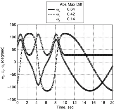
Figure 7. Test Case 1, Body A: Body axes angular velocity components. POST2/CFE as circles, AUTOLEV as lines.

(38)

Figure 8. Test Case 1, Body B: Body axes angular velocity components. POST2/CFE as circles, AUTOLEV as lines.

For t = 0 to 10 sec, when the bodies are connected, the angular velocity of each body is equal to that of the combined body. After release, the angular velocities vary such that total angular mo-mentum of body A and B remains constant and equal to that of the combined body. The change in the angular velocity components of body B are more noticeable than those for body A because B

is smaller in size compared to body A. Further, for body B, the moments of inertia about x and y

body axes were selected to be equal so that

= − = 0 (95) As a result, remains constant after release.

Figures 9 and 10 show the main results of the CFE method, which are the constraint forces and torques (moments). As said previously, these constraint forces/torques are applied as additional external loads for each body A and B within POST2. The results of this exercise show that the constraint forces/torques determined by CFE agree well with the AUTOLEV results.

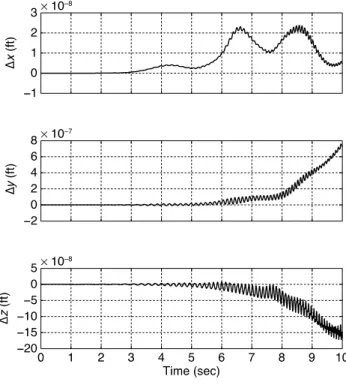
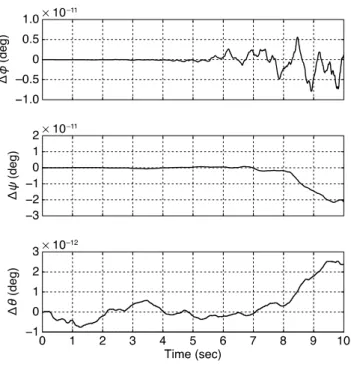
The relative joint displacement between the two bodies when they are supposed to stay con-nected is a basic metric to assess the accuracy of the POST2/CFE methodology. This parameter is computed as the position vector from ̅ to and should be ideally zero while the joint constraint is imposed for the first 10 sec. Hence, any deviation from zero is a measure of accuracy of the CFE algorithm. In the CFE algorithm the constraints are expressed at the acceleration level. However, as with all algorithms of this type, the constraints at the velocity and position levels are subject to numerical integration errors. Such errors depend on the step size in a fixed-step integration scheme or the error limits in a variable-step approach. Baumgarte stabilization (ref. 27) helps to control these errors from growing arbitrarily large during a simulation.

The choice of step size and Baumgarte factor (_η) for this problem was a reasonable balance be-tween CPU time and error buildup. Figure 11 shows the joint translational displacement as a