Florida International University
FIU Digital Commons
Department of Mathematics and Statistics
College of Arts, Sciences & Education
5-3-2013
Bayes multiple decision functions
Wensong Wu
Department of Mathematics and Statistics, Florida International University, [email protected]
Edsel A. Pena
University of South Carolina
Follow this and additional works at:
http://digitalcommons.fiu.edu/math_fac
Part of the
Physical Sciences and Mathematics Commons
This work is brought to you for free and open access by the College of Arts, Sciences & Education at FIU Digital Commons. It has been accepted for inclusion in Department of Mathematics and Statistics by an authorized administrator of FIU Digital Commons. For more information, please contact [email protected].
Recommended Citation
Wu, Wensong; Peña, Edsel A. Bayes multiple decision functions. Electron. J. Statist. 7 (2013), 1272--1300. doi:10.1214/13-EJS813. http://projecteuclid.org/euclid.ejs/1367585004.
Vol. 7 (2013) 1272–1300 ISSN: 1935-7524 DOI:10.1214/13-EJS813
Bayes multiple decision functions
Wensong Wu
Division of Statistics, Department of Mathematics and Statistics Florida International University, Miami, Florida 33199
e-mail:[email protected]
and Edsel A. Pe˜na Department of Statistics
University of South Carolina, Columbia, SC 29208 e-mail:[email protected]
Abstract: This paper deals with the problem of simultaneously making many (M) binary decisions based on one realization of a random data ma-trix X.M is typically large andX will usually haveM rows associated with each of theM decisions to make, but for each row the data may be low dimensional. Such problems arise in many practical areas such as the biological and medical sciences, where the available dataset is from mi-croarrays or other high-throughput technology and with the goal being to decide which among of many genes are relevant with respect to some phe-notype of interest; in the engineering and reliability sciences; in astronomy; in education; and in business. A Bayesian decision-theoretic approach to this problem is implemented with the overall loss function being a cost-weighted linear combination of Type I and Type II loss functions. The class of loss functions considered allows for use of the false discovery rate (FDR), false nondiscovery rate (FNR), and missed discovery rate (MDR) in assessing the quality of decision. Through this Bayesian paradigm, the Bayes multiple decision function (BMDF) is derived and an efficient algo-rithm to obtain the optimal Bayes action is described. In contrast to many works in the literature where the rows of the matrixXare assumed to be stochastically independent, we allow a dependent data structure with the associations obtained through a class of frailty-induced Archimedean copulas. In particular, non-Gaussian dependent data structure, which is typical with failure-time data, can be entertained. The numerical imple-mentation of the determination of the Bayes optimal action is facilitated through sequential Monte Carlo techniques. The theory developed could also be extended to the problem of multiple hypotheses testing, multiple classification and prediction, and high-dimensional variable selection. The proposed procedure is illustrated for the simple versus simple hypotheses setting and for the composite hypotheses setting through simulation stud-ies. The procedure is also applied to a subset of a microarray data set from a colon cancer study.
Keywords and phrases:Archimedean copula, Bayesian framework, de-cision theoretic framework, false discovery rate, frailty, multiple testing, sequential Monte Carlo.
Received December 2012.
1. Introduction
The advent of computer-automated high-throughput data-gathering technology, epitomized by the microarray, has led to the generation of so-called “large M, small n” data sets, which are those characterized by a large number, M, of variables (hereon called genes for historical reasons), which are observed or measured on a relatively small number, n, of subjects or units. Examples of such data sets in different scientific fields could, for instance, be found in [10] and [6].
For such data sets a typical goal is to choose an action,am, associated with genem, from a set of possible actions,Am, for each of theM genes. For example,
in a two-group microarray data set, one may want to decide, for each gene, whether it is differentially expressed between the two groups (action is a= 1), or whether it is not differentially expressed between the two groups (action is
a = 0). This situation corresponds to the problem of simultaneously testing multiple pairs of null and alternative hypotheses.
In this paper we shall focus on these two-point action spaces for each of the genes, that is, those withAm={0,1}. Of interest therefore is to choose a vector
of actions
a= (a1, a2, . . . , aM)T∈ A={0,1}M
based on the observed “largeM, smalln” data set. For themth gene there will be associated aθm ∈ {0,1}, which is unknown, representing thecorrect action to take. Thus, for the M genes there will be an unknown vector
θ= (θ1, θ2, . . . , θM)T∈Θ ={0,1}M
representing the vector of actions thatoughtto be taken. Thisθwill be referred to as thestate of reality. In light of this state of reality vectorθ, a chosen action vectorawill have consequences quantified through a loss. That is, there will be a mapping
(a,θ)7→L(a,θ)
where L(a, θ) is the loss that is incurred with the action a when reality is θ. Such a loss must take into account the loss incurred when the action isa = 1 when reality is θ = 0, called a Type I error, as well as the loss incurred when the action is a = 0 when reality isθ = 1, called a Type II error. There could be a variety of ways of measuring the overall Type I and Type II errors in such multiple decision problems, which will be formally described in Section 2.
These multiple decision problems appertaining to such “large M, small n” data sets lend naturally to a decision-theoretic framework discussed in more detail in Section 2. In addition to this decision-theoretic framework, we imple-ment a Bayesian approach to decision-making by putting a prior probability distribution on the unknown state of reality θ. Coupled with the appropriate loss function, we obtain the Bayes multiple decision action. To achieve this, we obtain the mathematical form of the Bayes multiple decision function, abbre-viated BMDF, and describe an efficient computational implementation of this BMDF under varied combinations of loss functions and data structures.
A decision-theoretic and a Bayesian approach to these multiple decision problems with high-dimensional data is certainly not new as can be seen in [15, 21, 20, 4, 3, 17]. Other approaches are in [22, 23] and [18]. See also the monograph [7]. An innovative major contribution of this paper is the use of a general class of loss functions that encompasses many of the loss functions that have been used in earlier works, thereby leading to a unified treatment of the multiple decision problem. For instance, the general class of loss functions introduced in Section 2 includes as special cases those that involve false posi-tives and false negaposi-tives as well as the commonly-used false discovery rates and false nondiscovery rates. Another major contribution is an efficient algorithm for computationally finding the Bayes multiple decision action, an algorithm that has computational order of at mostO(M2logM). Many papers have dealt with
the situation where the observables from each of the genes are stochastically in-dependent. We go beyond this usual assumption by incorporating dependencies among these observables, with the dependence structure induced by frailty-type models, which also takes the form of Archimedean copulas. This dependent modeling approach utilizes ideas from survival analysis where frailty and copula models have been used to model associations (see, for instance, [11]).
The statistical models governing these multiple decision problems in fact possess more complications than the simplistic description above. This is so since, even though the parameter of main interest is the state of reality vector θ, there will be unknown model parameters that are present which are nuisance, and we need to deal with them in constructing Bayes multiple decision functions and specifying prior probabilities. In our development of the BMDF we therefore first consider the situation of a simple null hypothesis versus a simple alternative hypothesis setting, wherein the distributional model for the random observable for the mth gene is completely known under either θm = 0 or θm = 1. We then utilize the results for this setting to solve the problem for a composite null hypothesis versus a composite alternative hypothesis setting, which are settings with nuisance parameters. An interesting development is the use of Sequential Monte Carlo (SMC) techniques to numerically approximate the Bayes multiple decision action especially in the presence of associations among the observables and in the prior probability specification.
We outline the contents of this paper. In Section 2 we will introduce the mathematical setting and elements of the multiple decision problem, including the general class of loss functions. Section3 will demonstrate the general form of the BMDF along with a computationally efficient algorithm of finding this BMDF in both simple and composite hypotheses testing settings. Section 4
will give the expressions of the BMDF under three concrete loss functions. We will introduce the frailty-based dependent data models in Section 5, and in Section 6 we will discuss computational aspects of the posterior calculations under the dependent models, and give algorithms using Sequential Importance Sampling (SIS). In Section 7 we will illustrate the BMDF in some concrete multiple decision problems, and compare the performance with currently used procedures via simulation studies. We will also apply the BMDF to a subset of a microarray data set. We will conclude the paper in Section8with some remarks.
2. Elements of decision theory
2.1. Multiple decision problem
Let (Ω,F,P) be a basic statistical model withPbeing a collection of probability measures on (Ω,F). Form= 1,2, . . . , M, where M ≥1 is a known integer, let
Xm: (Ω,F)→(Xm,Bm), whereXm is some space and Bm is an associatedσ
-field of subsets ofXm. In applications,Xmrepresents the vector of observables
for the mth gene. Let X = (X1, X2, . . . , XM) : (Ω,F) → (X,B), where X = NM
m=1Xm is the product sample space and B is the associated product σ
-field. A realization X = x will be called a (sample) data. For any P ∈ P, the induced joint probability measure ofXisQ=PX−1, whereas the marginal
probability measure ofXm isQm=P X−1
m . LetQ={PX−1 :P ∈ P} denote
the collection of all probability measures ofXinduced byP. Consider a mapping
ϑ = (ϑ1, ϑ2, . . . , ϑM)T : Q → {0,1}M, where ϑm : Q → {0,1} only depends
on the mth marginal probability measure. In essence, the parameter of main interest is ϑ(Q) = θ = (θ1, θ2, . . . , θM)T, which takes values in the parameter
space Θ = {0,1}M. Observe that Q can be decomposed via Q = U
θ∈ΘQθ, where Qθ = {Q ∈ Q : ϑ(Q) = θ},∀θ ∈ Θ. Let a = (a1, a2, . . . , aM)T be an
action in the action spaceA={0,1}M. LetL◦:A × Q →Rbe a loss function such that L◦(a, Q) =L(a,ϑ(Q)),∀a ∈ A,∀Q∈ Q, where L:A ×Θ→R is a loss function belonging to a class Ldiscussed in Section2.2.
Since we are implementing a Bayesian framework we may restrict the space of decision functions, D, to be nonrandomized [2]. Such decision functions are measurable maps δ from X to A with δ(x) = (δ1(x), δ2(x), . . . , δM(x)) being
the action taken when observed data is x. For a δ∈ D, its risk function (with respect to Q) is R◦(δ, Q) = X θ∈Θ Z X L(δ(x),θ)Q(dx) I(ϑ(Q) =θ).
We shall assume that for anyθ ∈ Θ,Qθ is an identifiable parametric class given by Qθ ={Qθ(·;γθ) :γθ∈Γθ}, whereγθ is a nuisance parameter. This implies that Q is an identifiable model with respect to the parameter (θ, γθ) which belongs to the enlarged parameter space Θ◦=∪
θ∈Θ[{θ} ×Γθ]. Then, for anyδ∈ DandQ∈ Q, the risk function is given by
R◦(δ, Q) = X θ∈Θ R(δ,(θ, γθ))I(ϑ(Q) =θ, Q=Qθ(·;γθ)), where R:D ×Θ◦→Ris given by R(δ,(θ, γθ)) =EX∼Qθ(·;γθ)L(δ(X),θ) = Z X L(δ(x),θ)Qθ(dx;γθ). Furthermore, the decomposition ofQ becomes
Q= ] θ∈Θ n Qθ(·;γθ) :ϑ(Qθ(·;γθ)) =θ, γθ∈Γθ o .
A prior probability measure on Q can be constructed by specifying a prior probability measure on (Θ◦, σ(Θ◦)), where σ(Θ◦) is the σ-field generated by a semi-ringC={{θ}×Cθ:Cθ∈σ(Γθ),θ∈Θ}withσ(Γθ) aσ-field on Γθ. Define a probability measure Π∗ onC such that for anyθ
0∈Θ and anyCθ0 ∈σ(Γθ0),
Π∗(θ=θ0, γθ∈Cθ0) = Π(θ0)
Z
Cθ0
Pθ0(dγθ0) = Π(θ0)Pθ0(Cθ0),
where Π(·) is a prior probability measure on Θ andPθ(·) is a prior probability measure on Γθ. This induces, by Caratheodory’s extension theorem, a prior probability measure Π◦ on (Θ◦, σ(C) = σ(Θ◦)). Since the elements of Q are identified by (θ, γθ), there is a one-to-one and onto mapping h: Θ◦→ Q with (θ, γθ)
h
↔ Qθ(·;γθ). Therefore, Π◦ determines a prior probability measure on (Q, σ(Q)), whereσ(Q) =h σ(Θ◦).The Bayes risk function of a decision function
δ∈ Dfor the prior Π◦ is defined via
rΠ◦(δ) =EQ∼Π◦R◦(δ, Q) = Z Θ Z Γθ R(δ,(θ, γθ))Pθ(dγθ)Π(dθ). A decision functionδ∗ is called a Bayes multiple decision function (BMDF) if
δ∗= arg min
δ∈D
rΠ◦(δ).
The multiple decision problem is to find the BMDF, which is the Bayes optimal procedure for choosing theM-dimensional action vector. More practically, there is the issue of finding the Bayes optimal action, which is the realization ofδ∗, in a computationally efficient manner.
2.2. Class of loss functions
The value L(a,θ) of a loss function L : A ×Θ→ R quantifies the error that is committed when action a is chosen and θ is the state of reality. We shall consider a class of cost-weighted loss functions whose members are of form
L(a,θ) =C0L0(a,θ) +C1L1(a,θ), (1)
where C0 ≥ 0 and C1 ≥0 are pre-determined costs for loss functions L0 and L1, respectively. L0 will quantify the loss from the Type I errors, whereas L1
will quantify the loss from the Type II errors. The general forms ofL0and L1
are, respectively,
L0(a,θ) = [α0(aT1)g0(a)]T[β0(θT1)h0(θ)]; L1(a,θ) = [α1(aT1)g1(a)]T[β1(θT1)h1(θ)],
where αj : R → R, βj : R → R, gj : A → A, and hj : Θ →Θ for j = 0,1. We assume further that, for j = 0,1, gj is τj-invariant with respect to the
Table 1
Some examples of loss functions used in this paper. FP and FDP are Type I loss functions, while FN, MDP, FNP and AMDP are Type II loss functions
Descriptive Name Abbreviation L(a,θ)
False Positive Proportion FP a
T(1−θ)
M
False Negative Proportion FN (1−a)
Tθ
M
False Discovery Proportion FDP a
T(1−θ)
(aT1)∨1
Missed Discovery Proportion MDP (1−a)
Tθ
(θT1)∨1
False Nondiscovery Proportion FNP (1−a)
Tθ
((1−a)T1)∨1
Adjusted Missed Discovery Proportion AMDP (1−a)
Tθ
(θT1) + 1
sub-action space Ak ≡ {a∈ A : aT1=k} for k ∈ M ≡ {0,1, . . . , M}, in the
sense that there exists a mapping τj : M → M associated with gj such that
a∈ Akimpliesgj(a)∈ Aτj(k). Examples ofτ include the identity mapping with τ0(k) =kand alsoτ1(k) =M−k. Theng0withg0(a) =aisτ0-invariant, while
g1 with g1(a) =1−a is τ1-invariant. With a∨b = max(a, b), some examples
of loss functionsL0 andL1 onA ×Θ are given in Table1.
Besides the aforementioned properties ofL0andL1, we also assume thatL0
andL1possess a complementarity property given by
g1(a) =a0−A1g0(a)
for some a0 ∈ Aand withA1 >0. In the multiple hypotheses testing settings
considered in this paper, we will haveA1= 1,a0=1, andg0(a) =a. This
prop-erty describes a relation betweenL0 and L1 which indicates that they are loss
functions having complementary behaviors. For example, FP and FDP are pro-portions of false discoveries, where a discovery at the mth coordinate is having
am= 1, whereas FN, MDP, and FNP are proportions of false nondiscoveries. In the sequel, we will consider the pairs (FP, FN), (FDP, FNP), and (FDP, MDP) for (L0, L1) in the multiple decision problem. The cost constantsC0andC1will
generally be determined by the decision maker or subject matter specialist, and they reflect the consequences of false discoveries and false nondiscoveries.
2.3. Multiple testing problems 2.3.1. Simple hypotheses setting
The simple-versus-simple multiple hypotheses testing problem is a particular case of this multiple decision problem. Suppose that the marginal probability distribution of Xm satisfies Qm ∈ {Qm0, Qm1} with Qm0 6= Qm1, and the
parameter vector is θ = (I(Qm = Qm1), m = 1,2, . . . , M). We may consider
simultaneously the M pairs of simple versus simple hypotheses Hm0 : Qm = Qm0 versus Hm1 : Qm = Qm1 for m = 1,2, . . . , M. In this case, for m =
1,2, . . . , M, θm = 1(0) indicates whether Hm1 is (not) true, and the action
am= 1(0) means rejecting (not rejecting) Hm0.
Usually, independent Bernoulli priors are assigned toθ. Letπm0, πm1∈(0,1)
be such that πm0+πm1 = 1 form = 1,2, . . . , M. The prior probability mass
function πonθ is specified by π(θ) = M Y m=1 πm1−0θmπmθm1I(θm∈ {0,1}). (2)
In this situation, the Bayes risk function of a decision functionδfor a prior mass function πofθ is
rπ(δ) =Eθ∼πEX∼QθL(δ(X),θ),
associated with a loss functionL∈ L, whereQθis the joint probability function ofX, givenθ, and whosemth marginal distribution function isQm=Qmθm. 2.3.2. Composite hypotheses setting
Suppose thatQm, the marginal distribution ofXm, is in a class of distributions
Qm given byQm ={Qm(·;γm, ξm) : γm ∈Γm, ξm ∈Ξm}; Assume, for m =
1,2, . . . , M, Γm= Γm0∪Γm1 and Γm0∩Γm1=∅. ThenQmhas two subclasses
denoted by
Qm0={Qm(·;γm, ξm) :γm∈Γm0, ξm∈Ξm}
Qm1={Qm(·;γm, ξm) :γm∈Γm1, ξm∈Ξm}.
Consider theM pairs of composite hypothesesHm0 : Qm∈ Qm0 versusHm1: Qm ∈ Qm1, for m = 1,2, . . . , M. Note that Γm0, Γm1, or Ξm could be the
same for all m, though in general they may be different. Let θ = (I(Qm ∈ Qm1), m= 1,2, . . . , M) = (I(γm∈Γm1), m= 1,2, . . . , M)∈Θ ={0,1}M, γ=
(γ1, γ2, . . . , γM)∈ Γ ≡NMm=1Γm, and ξ = (ξ1, ξ2, . . . , ξM) ∈Ξ ≡NMm=1Ξm.
Also, for anyθ∈Θ, let Γθ≡NMm=1Γmθm. Then the extended parameter vector
is
(θ,γ,ξ)∈Θ◦≡ ]
θ∈Θ
{{θ} ×Γθ×Ξ}, (3) whereθ∈Θ is the parameter of main interest in the multiple decision problem, while (γ,ξ)∈Γ×Ξ are nuisance parameters. Note that the value ofγdetermines
the value of θ, but we only want to determine whetherγm∈Γm0or γm∈Γm1
rather than estimating the exact values of γms. The parameterθ ∈Θ and the actiona∈ Ahave the same interpretation in this composite hypotheses testing problem as in the simple-vs-simple hypotheses setting.
Assume that the prior distribution on the enlarged parameter space Θ◦ is
π(θ,γ,ξ) =
M Y
m=1
(πm0pm0(γm, ξm))1−θm(πm1pm1(γm, ξm))θm, (4)
wherepm0andpm1are prior densities on Γm0×Ξmand Γm1×Ξm, respectively,
and with πm0, πm1 ∈ (0,1) and πm0+πm1 = 1. The Bayes risk function of
a decision function δ for a prior density π of (θ,γ,ξ) associated with a loss function L∈ Lis
rπ(δ) =E(θ,γ,ξ)∼πEX∼Qθ(·;γ,ξ)L(δ(X),θ),
where Qθ(·;γ,ξ) is the joint probability function of X, given (θ,γ,ξ), and the marginal probability measures are Qm = Qm(·;γm, ξm), m = 1,2, . . . , M. To indicate that the marginalQm∈ Qmθm, we shall denote it byQmθm(·;γm, ξm).
3. Bayes multiple decision functions
3.1. BMDF in simple hypotheses
Let π(·) be a prior probability mass function of θ ∈ Θ. Then the Bayes risk function ofδfor the priorπis given by
rπ(δ) =Eθ∼πR(δ,θ) =EθEX|θL(δ(X),θ) =EXEθ|XL(δ(X),θ), where Eθ|X is the expectation with respect to the posterior distribution of θ givenX. Fora∈ AandX=x∈ X, define the posterior expected loss by
˜
L(a,x) =Eθ|X=xL(a,θ), (5)
and denote the optimal action whenX=xby
a∗(x) = arg min a∈A ˜ L(a,x). (6) Then the BMDF is δ∗(X) =a∗(X). (7)
Notice that finding the optimal actiona∗, and thus the BMDFδ∗, via equa-tion (6) involves searching for the minimizer of the function ˜L among all 2M
elements of A. When M is relatively large, the number of operations required to find the optimal action (hereon called the searching order) is of orderO(2M),
which would be practically infeasible to implement. Furthermore, note that this computational problem does not yet include the problem of computing the pos-terior distribution of θgivenX=x.
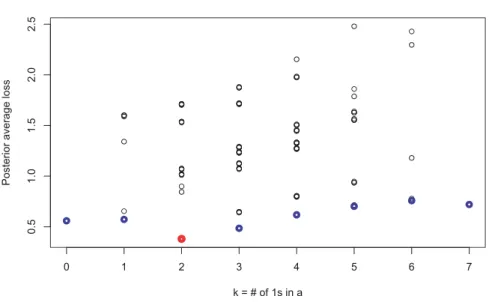
0 1 2 3 4 5 6 7 0. 5 1. 0 1. 5 2. 0 2. 5 k = # of 1s in a
Posterior average loss
Fig 1. Graph of k = aT1 versus the posterior average loss functions when M = 7 for a
simulated data. Blue circles are restricted optimal actions within sub-action spaces; Red circle is the optimal action. Black circles represent all other actions.
The idea for obtaining a computationally efficient algorithm to find the opti-mal action is to first find the restricted optiopti-mal action over the sub-action space
Ak ={a ∈ A:aT1=k} for each k∈ M, and then to find the optimal action
among these restricted optimal actions. Figure1 shows an example for a simu-lated data whenM = 7. The 2M = 128 actions in the action spaces are stratified
into eight sub-action spaces according to k =aT1= 0,1, . . . ,7. The search of each restricted optimal action with the least ˜Lwithin each sub-action space is computationally easier because of the form of the loss function, so that a direct search of the optimal action with the least ˜L among all actions is not needed.
Before presenting the results, we first define some relevant quantities that will be used. With the notation of the lossL∈ L described in Section2.2, for
k∈ M, let
d0(k,x) =C0α0(k)Eθ|X=x[β0(θT1)h0(θ)]; (8)
d1(k,x) =C1α1(k)Eθ|X=x[β1(θT1)h1(θ)]; (9)
e(k,x) =d0(k,x)−A1d1(k,x); (10)
and letr(k,x) = (rm(k,x), m= 1,2, . . . , M) be the rank vector ofe(k,x). Also, define H(k,x) =aT 0d1(k,x) + M X m=1 I(rm(k,x)≤τ0(k))em(k,x), (11)
where we recall that τ0 : M → M is a mapping such that a ∈ Ak implies
Theorem 1. For a multiple decision problem with loss function L ∈ L and prior probability mass function π onθ, let k∗:X → M be defined via
k∗(x) = arg min
k∈M
H(k,x), x∈ X,
where H :M × X → Ris defined in (11). Then the BMDF is of the form (7) with a∗(x) satisfying g0(a∗(x)) = I{rm(k∗(x),x)≤τ0(k∗(x)}, m= 1,2, . . . , M . (12)
The searching order for obtaining the Bayes optimal action associated with the BMDF is no more than O(M2logM).
Proof. Associated with the loss function L, ˜L defined in equation (5) has a specific form given by
˜ L(a,x) = 1 X j=0 Cj[αj(aT1)g j(a)]TEθ|X=x[βj(θT1)hj(θ)]. RestrictingaonAk, ˜ L(a,x) =g0(a)Td0(k,x) +g1(a)Td1(k,x) =aT0d1(k,x) +g0(a)T[d0(k,x)−A1d1(k,x)] =aT0d1(k,x) +g0(a)Te(k,x),
where d0(k,x),d1(k,x), ande(k,x) are as defined in (8)-(10).
Since for a ∈ Ak, g0(a)T1 = τ0(k), the optimal action on Ak, denoted by
a∗
k(x), which minimizes ˜L(a,x) fora∈ Ak, therefore satisfies
g0(a∗k(x)) = I{r1(k,x)≤τ0(k)}, I{r2(k,x)≤τ0(k)}, . . . , I{rM(k,x)≤τ0(k)} T ,
where we recall that, form= 1,2, . . . , M,rm(k,x) is the rank ofem(k,x) among the elements ofe(k,x),m= 1,2, . . . , M. Thus,
˜ L(a∗k(x),x) =aT0d1(k,x) + M X m=1 I(rm(k,x)≤τ0(k))em(k,x),
which equals the function H(k,x). Therefore, for the k∗(x) in the statement of Theorem 1, a∗k∗(x)(x) minimizes ˜L(a,x) over all actionsa∈ A. The optimal action, givenX=x, is thereforea∗(x) =a∗
k∗(x)(x), which satisfies (12).
For the computational order of the algorithm, observe that fork∈ M, in or-der to finda∗
k(x), it is only necessary to know which are theτ0(k) smallest among
Upon obtaining a∗
k(x), one only needs to search the minimum of H(k,x) for k∈ M. Therefore, the searching order is bounded byPM
k=1O(M+τ0(k) logM).
The worst-case scenario is whenτ0(k)≡M, k= 0,1, . . . , M, which leads to an
upper bound ofO(M2logM).
Observe that the searching order ofO(M2logM) is a considerable
improve-ment overO(2M). This is due to the special form of the loss function and the
nature of the parameter space, action space, and multiple decision function space. In a lot of cases, including the specific pairs of loss functions discussed in Section4, the searching order may still be lower thanO(M2logM).
Observe also that in the BMDF described in Theorem1, we need to obtain the posterior expectation of form Eθ|X=x[β(θT1)h(θ)]. Recall that Xm, given θ, has the marginal distributionQmθm. We assume for now that theXms, given θ, are independent form= 1,2, . . . , M. In general, we may also model theXms to be dependent as will be discussed in Section5, in which case the computation of the posterior expectation will be discussed in Section6. Denote the density of
Qmθmbyqmθm. Suppose an independent prior distribution of the form described in (2) is used. Then, the posterior distribution ofθhas theθms also independent, with πm(θm|x) = πmθmqmθm(xm) πm0qm0(xm) +πm1qm1(xm), m= 1,2, . . . , M. Therefore, Eθ|x[β(θT1)h(θ)] = X θ∈Θ β(θT1)h(θ) M Y m=1 πmθmqmθm(xm) πm0qm0(xm) +πm1qm1(xm) .
In general, this is a sum of |Θ| = 2M terms. A particular case is E(θ|x) =
(E(θ1|x), E(θ2|x), . . . , E(θM|x)) where, form= 1,2, . . . , M,
E(θm|x) =P(θm= 1|x) = πm1qm1(xm)
πm0qm0(xm) +πm1qm1(xm).
An important aspect to note is that in general, each component of the poste-rior expectationEθ|x[β(θT1)h(θ)] is needed to obtain the BMDF, so that each component ofδ∗may depend onallcomponents ofX. This makes the BMDF a compounddecision function [23]. In essence the decision for themth component borrows information from the other components, or as mentioned in [8], the decision makes use of direct evidence from themth component of the data as well as indirect evidence from the other components.
3.2. BMDF in composite hypotheses
Letπ be a prior density function on the enlarged parameter space Θ◦ (see (3) on page1278). Then the Bayes risk of a decision functionδ∈ Dis given by
Observe that the final form of the Bayes risk is exactly the same as in the simple-vs-simple hypotheses setting. This implies that the results in Theorem1
apply directly. However, since the parameter space where the prior distribution is defined is enlarged, the posterior expectation Eθ|x[L(δ(x),θ)] in the Bayes risk, orEθ|x[β(θT1)h(θ)] in Theorem1is now taken with respect to themarginal posterior distribution of θ, given X=x.
Assume theXms, givenθ, are independent, form= 1,2, . . . , M. Denote the density of Qm(·;γm, ξm), under Hmθm, by qmθm(·;γm, ξm). If an independent prior of the form in (4) is assigned, then the marginal posterior distribution of θ also makesθms independent, with
πm(θm|x) = πmθmqmθm˜ (xm) πm0qm˜ 0(xm) +πm1qm˜ 1(xm) , where ˜ qmθm(xm) = Z Γmθm Z Ξm pmθm(γm, ξm)qmθm(xm;γm, ξm)dξmdγm. (13) Therefore, Eθ|x[β(θT1)h(θ)] = X θ∈Θ β(θT1)h(θ) M Y m=1 πmθmqmθm˜ (xm) πm0qm˜ 0(xm) +πm1qm˜ 1(xm).
In particular, E(θ|x) = (E(θ1|x), E(θ2|x), . . . , E(θM|x)) where, for m = 1,2, . . . , M,
E(θm|x) = πm1qm˜ 1(xm)
πm0qm˜ 0(xm) +πm1qm˜ 1(xm) .
Notice that the integral in ˜qmθm(xm) may not be in closed form. Thus Monte Carlo techniques may be needed even in this independent setting to approxi-mately compute ˜qmθm(xm) and henceE(θm|x). Similarly to the simple-vs-simple hypotheses setting, the BMDF in this composite hypotheses setting is com-pound.
4. Loss functions: Special cases
4.1. Combination of FP and FN loss functions Consider the loss function
L(F P,F N)(a,θ) =C0LF P(a,θ) +C1LF N(a,θ) =C0a
T(1−θ)
M +C1
(1−a)Tθ
M ,
where LF P and LF N are the false positive proportion and false negative pro-portion.
This is the loss function that has been studied extensively in previous pa-pers. It is clear that the optimal action minimizing ˜L(F P,F N)isa∗(F P,F N)(x) =
((a∗(F P,F N)(x))m, m= 1,2, . . . , M),where, form= 1,2, . . . , M, (a∗(F P,F N)(x))m=I E(θm|x) 1−E(θm|x) > C0 C1 =I E(θm|x)> C0 C0+C1 .
The corresponding BMDF δ∗ is such that δ∗(X) = a∗(X). This BMDF is of intuitive form in that the decision on each component is based only on
E(θm|x) = P(θm = 1|x) and the threshold is just C0/(C0+C1), though it
should be pointed out thatE(θm|x) may depend on all the data. Note that, when
M = 1, this is just the Bayes test corresponding to a C0/C1-loss function [5].
4.2. Combination of FDP and FNP loss function Consider the loss function
L(F DP,F N P)(a,θ) = C0LF DP(a,θ) +C1LF N P(a,θ) = C0a T(1−θ) (aT1)∨1 +C1 (1−a)Tθ ((1−a)T1)∨1,
where LF DP and LF N P are the false discovery proportion and the false non-discovery proportion. Note that for this L ∈ L, h0(θ) = 1−θ, h1(θ) = θ,
g0(a) = a, a0 = 1, A1 = 1, andτ0(k) = k, α0(k) = 1/(k∨1), and α1(k) =
1/[(M−k)∨1]. This loss function has also been studied previously.
Let (φ(1)(x), φ(2)(x), . . . , φ(M)(x)) denote the ordered vector associated with E(θ|x). Then, in Theorem1, we have
H(k,x) =C1 PM m=1φm(x) (M −k)∨1 + " C0 Pk i=1(1−φ(M−i+1)(x)) k∨1 −C1 Pk i=1φ(M−i+1)(x) (M−k)∨1 # =C0 Pk i=1(1−φ(M−i+1)(x)) k∨1 +C1 PM i=k+1φ(M−i+1)(x) (M−k)∨1 . Letting k∗(x) = arg min
k∈M H(k,x),by Theorem1 the optimal action is
a∗(F DP,F N P)(x) = (I(rm(k∗(x),x)≤k∗(x)), m= 1,2, . . . , M)
= (I(rank(E(θm|x))≥M −k∗(x) + 1), m= 1,2, . . . , M) = (I(M+ 1−rank(P(θm= 1|x))≤k∗(x)), m= 1,2, . . . , M).
Notice that for allk= 1,2, . . . , M−1,H(k,x) depends only on the ordered vector of E(θ|x), which means that in order to select k∗(x) we only need to sort E(θ|x) once. Also, the optimal action only requires the rank vector of
E(θ|x) afterk∗(x) has been obtained. Therefore, the searching order is reduced toO(MlogM).
For this case, the posterior means of the θm’s are still the main basis of choosing the optimal actions, but in contrast to the previous case, the decision at any particular component depends onallposterior means. One may initially conclude that the Bayes multiple decision function does not depend on the magnitudes of theE(θm|x), but rather only on their relative ranks. However, this isnotthe case since their magnitudes are actually needed to determine k∗(x).
Observe also that this Bayes optimal action has similarities to the Benjamini-Hochberg (BH) procedure [1], since it can be considered as a step-up procedure which compares ordered posterior probabilities thatθm= 1 to a data-dependent critical cutoff value, whereas the BH procedure also compares ordered p-values to a data-dependent critical cutoff value. Analogous observations of the similarities of Bayes procedures to the BH procedure have also been pointed out in [14] and [4].
4.3. Combination of FDP and MDP loss functions Consider the loss function
L(F DP,M DP)(a,θ) =C0LF DP(a,θ) +C1LM DP(a,θ) =C0 aT(1−θ) (aT1)∨1 +C1 (1−a)Tθ (θT1)∨1,
where LF DP andLM DP are the false discovery proportion and the missed dis-covery proportion. Analogously for the pair of (FDP, FNP), h0(θ) = 1−θ, h1(θ) = θ,g0(a) =a, a0 =1, A1 = 1, andτ0(k) =k, α0(k) = 1/(k∨1), and α1(k) = 1. Let e(k,x) =C0 k E(1−θ|x)−C1E θ (θT1)∨1 x ,
and denote by (e(1)(k,x), e(2)(k,x), . . . , e(M)(k,x)) the ordered vector ofe(k,x).
Then H(k,x) =C11TE θ (θT1)∨1|x + k X i=1 e(i)(k,x) and k∗(x) = 0 if min k∈M\{0} k P i=1 e(i)(k,x)>0 arg min k∈M\{0} k P i=1 e(i)(k,x) otherwise .
By Theorem1, the optimal Bayes action is
a∗(F DP,M DP)(x) = (I(rank(em(k∗(x),x))≤k∗(x), m= 1,2, . . . , M).
Observe thata∗(x) andk∗(x) depend on the values and ranks of ˜em(k,x) fork∈
M. The searching order in this case isO(M2logM). It can be shown that when
the posterior probability distribution of θ specifies independent components, the searching order is reduced toO(MlogM).
4.4. Discussion of choice of loss functions
As shown in this section, different loss functions lead to different forms of the BMDF, that is, given the same data x, it is possible that different Bayes op-timal actions will arise by varying the loss functions. The loss function pair of
(F P, F N) is the most straight-forward as it is equivalent to counting the
num-ber of errors. Some theoretical studies, such as [3], have shown that the BH false discovery rate controlling procedure possesses an asymptotic Bayes opti-mality under this loss function. However, if the goal is to minimize the Bayes risk using a loss function induced by the F DP, then the loss function pair of
(F DP, F N P) or (F DP, M DP) will be more appropriate since they are both
weighted sums ofF DP and a specific type II error loss function. In addition, as shown in this section, the BMDF associated with these two loss functions have a flavor similar to the BH procedure. Computationally, these two have the same searching order once the necessary posterior expectations have been calculated. However, the BMDF associated with (F DP, M DP) requires the posterior ex-pectation ofθ/[(θT1)∨1], which involves the entire vectorθ. As we will discuss in the sections dealing with sequential Monte Carlo procedures, the computa-tion of this posterior expectacomputa-tion is relatively more extensive and less stable. Thus, in practice, an adjusted version ofM DP, theAM DP indicated in Table
1, is recommended. Even with the use of the AM DP, the computational cost is still higher compared to the case where the (FDP, FNP) pair is used.
5. Dependent data structure
In Section3, formulas of the posterior expectations are given under the assump-tion that theXm’s,m= 1,2, . . . , M, are independent. However, in various situ-ations this assumption may not be realistic. Recall in section2.1thatQθ(·;γθ) is the probability measure of X, given (θ, γθ), with ϑ(Qθ(·;γθ)) = θ. In this section, we describeQθ(·;γθ) that allows for dependencies among theXms inX. In the simple hypotheses setting, the goal is to specifyQθ, the joint probabil-ity distribution ofXgivenθ, such that the marginal probability distribution of
Xm isQm=Qmθm. LetM0(θ) ={m∈ {1,2, . . . , M}:θm= 0} andM1(θ) =
{m∈ {1,2, . . . , M}:θm= 1}. Assume thatXM0(θ)≡ {Xm:m∈ M0(θ)} is a
collection of independent random vectors, and XM1(θ) ≡ {Xm:m ∈ M1(θ)}
is a collection of possibly dependent vectors, and the collections XM0(θ) and
XM1(θ)are independent of each other. Borrowing from survival analysis ideas,
we assume that the dependence structure of the collection XM1(θ) is induced
by an unobserved frailty variableZ. We assume that, conditionally on Z =z,
XM1(θ)are independent. Specifically, assume that
Qθ \ m∈M1(θ) [Xm∈Bm] Z =z = Y m∈M1(θ) [ ˘Qm(Bm)]z,
for allBm∈ Bm,m∈ M1(θ), where ˘Qm’s are some distributions on (Xm,Bm)’s,
have been widely used in survival analysis, where the frailty variable is used to account for hidden heterogeneity. We use this idea in the multiple decision setting, where the frailty variable is used to model the possible common feature for genes in the true alternative collection, for example, those genes that are differentially expressed across treatment groups.
The joint distribution ofXM1(θ) is
Qθ \ m∈M1(θ) [Xm∈Bm] = Z Z Y m∈M1(θ) [ ˘Qm(Bm)]zG(dz), (14)
for all Bm ∈ Bm, m ∈ M1(θ). Recall that in the simple-vs-simple multiple
hypotheses testing setting, under Hm1,Xm∼Qm1 marginally. So the
distribu-tions ˘Qm,m ∈ M1(θ), should be such that these conditions are satisfied. Let
LG be the Laplace transform of the distribution functionG, that is,
LG(u) = Z
Z
e−uzG(dz),∀u∈R.
LetM1≡ |M1(θ)|. The following result gives the joint distribution of the
depen-dent collectionXM1(θ) in terms of the collection of the marginal distributions
{Qm1:m∈ M1(θ)}under this frailty-based model.
Proposition 1. The frailty-based model described in (14) is anM1-dimensional
Archimedean copula CG such that
Qθ \ m∈M1(θ) [Xm∈Bm] =CG(Qm1(Bm), m∈ M1(θ))
for all Bm∈ Bm, whereCG: [0,1]M1→[0,1]is defined via CG(u1, u2, . . . , uM1) =LG M1 X m=1 L−G1(um) ! .
Proof. According to the model, marginally form∈ M1(θ) and allBm∈ Bm,
Qm1(Bm) = Z Z ˘ Qm(Bm)zG(dz) = Z Z exp −z −log ˘Qm(Bm) G(dz) =LG(−log ˘Qm(Bm)).
Thus ˘Qm(Bm) = exp(−L−G1(Qm1(Bm)). So,
Qθ \ m∈M1(θ) [Xm∈Bm] = Z Z Y m∈M1(θ) (exp(−L−G1(Qm1(Bm))))zG(dz)
= Z Z exp − X m∈M1(θ) L−G1(Qm1(Bm)) ·z G(dz) =LG X m∈M1(θ) L−G1(Qm1(Bm)) .
To showCG is an Archimedean copula, it is sufficient to show that the func-tion L−G1 is a strict generator of a copula, which is that it is a continuous strictly decreasing convex function from [0,1] to [0,∞] with L−G1(1) = 0 and
L−G1(0) = ∞ [16]. But these are straight-forward to verify using properties of the Laplace transform.
Thus, a frailty-induced dependent full data model is given by
Qθ M \ m=1 [Xm∈Bm] ! = Y m∈M0(θ) Qm0(Bm) CG h Qm1(Bm), m∈ M1(θ) i , (15) for allBm∈ Bm,m= 1,2, . . . , M. Notice that the distribution functionGmay
have nuisance parameters, say, G(·) = G(·,υ), where υ ∈ Υ. In this case, to calculate the posterior expectations, a prior on Υ will also be needed.
In the composite hypotheses testing setting, we are to specifyQθ(·;γ,ξ), the joint probability distribution ofXgiven (θ,γ,ξ), such that the marginal prob-ability distribution ofXmis Qm=Qmθm(·;γm, ξm). The result in Proposition
1is easily extended to get
Qθ \ m∈M1(θ) [Xm∈Bm];γ,ξ =CG h Qm1(Bm;γm, ξm), m∈ M1(θ) i ,
and the full data model is given by
Qθ M \ m=1 [Xm∈Bm];γ,ξ ! = Y m∈M0(θ) Qm0(Bm;γm, ξm) CG h Qm1(Bm;γm, ξm), m∈ M1(θ) i .
6. Sequential Monte Carlo
The applicability of the algorithm for finding the Bayes optimal action in Theo-rem1is contingent on an efficient way of calculating the posterior expectations
E(H(θ)|X=x) =X
θ∈Θ
where H(θ) takes the formβ(θT1)h(θ) and π(θ|x) is the posterior probability mass function ofθ, given datax. For example, the specific forms of theH func-tion desired in case of FDP and MDP loss funcfunc-tions areH(θ) =θ andH(θ) = θ
(θT1)∨1
. As pointed out in Sections3 and5, Monte Carlo integration is needed for approximating the posterior expectations. However, in the regular Importance Sampling (IS) algorithm [19], asM, the dimension ofθ, increases, the computational complexity of calculating the weights also increases. So it is important to consider a sequential application of the importance sampling methods [9]. Notice that the index m, which takes values 1,2, . . . , M, does not necessarily represent time or positions in an ordered sequence, and that the pro-posed dependent data structure is not necessarily a state space model as what is usually the case in sequential importance sampling applications. However, the sequential technique provides a visual solution through m = 1,2, . . . , M
which deals with the dimensionality and monitors the efficiency of the sampling procedure.
6.1. Simple hypotheses
Letπbe a prior probability mass function ofθ. Under the dependent data model described in (15), the desired posterior expectation is given by
I(x) =E(H(θ)|x) = P θ∈ΘH(θ)π(θ)Qθ(dx) P θ∈Θπ(θ)Qθ(dx) , where Qθ(dx) = Y m∈M0(θ) qm0(xm) × Y m∈M1(θ) qm1(xm) cG(Qm1(xm), m∈ M1(θ))dx,
with qm0 and qm1 being the density functions of Qm0 and Qm1, respectively,
and
cG(u1, u2, . . . , uM1) =
∂M1
∂u1∂u2. . . ∂uM1
CG(u1, u2, . . . , uM1)
is the copula density of CG. Consider an independent data-adaptive trial prob-ability mass functiongofθ given byg(θ) =g(θ|x) =QM
m=1gm(θm|xm),where,
form= 1,2, . . . , M,gm(θm|xm) is the marginal posterior ofθm, givenXm=xm. This is a Bernoulli distribution of form
gm(θm|xm)∝πm(θm)qm0(xm)1−θmqm1(xm)θm, (16)
where πm(θm) is the marginal prior probability of θm. Denote by x1:m =
prior distribution ofθ can be written asπ(θ) =QM
m=1πm(θm|θ1:m−1), where π1(θ1|θ1:0) is the marginal distribution ofθ1, and form= 2,3, . . . , M,πm(θm|
θ1:m−1) is the probability ofθm, givenθ1:m−1, under the joint priorπ. Notice
that if πis independent, then πm(θm|θ1:m−1) =πm(θm). However, dependent
prior structures can also be constructed using frailty-induced models similarly to the dependent data structure, in which caseπm(θm|θ1:m−1) does not necessarily
reduce toπm(θm).
Letqθ1:m(x1:m) be the marginal density function ofX1:m, givenθ1:m, under
the dependent data structure proposed in (15). Since the dependent structure is induced by a frailty model, we have, for m = 2,3, . . . , M, qθ1:m(x1:m) = qθ1:m(xm|x1:m−1)·qθ1:m−1(x1:m−1), where qθ1:m(xm|x1:m−1) = qθ1:m(x1:m) qθ1:m−1(x1:m−1) = qm0(xm) ifθm= 0 qm1(xm) cG(Qt1(xt), t∈ M1(θ1:m)) cG(Qt1(xt), t∈ M1(θ1:m−1)) ifθm= 1. Thus, the full density of the data has the sequential form
qθ(x) =
M Y
m=1
qθ1:m(xm|x1:m−1) withqθ1(x1|x1:0) = 1.
So there is a recursive formula for calculating the importance weight function, given by
wm(θ1:m|x1:m) =wm−1(θ1:m−1|x1:m−1)um(θ1:m|x1:m),
where the increment
um(θ1:m|x1:m) = qθ1:m(xm|x1:m−1)π(θm|θ1:m−1) gm(θm|xm) satisfies um(θ1:m|x1:m) ∝ π(θm= 0|θ1:m−1) πm(θm= 0) ifθm= 0 cG(Qt1(xt), t∈ M1(θ1:m)) cG(Qt1(xt), t∈ M1(θ1:m−1)) ·π(θm= 1|θ1:m−1) πm(θm= 1) ifθm= 1 . (17)
Note that wM(θ1:M|x1:M) = w(θ|x), the importance weight function. These
results will now enable us to sample particles and calculate the importance weights in a sequential manner.
The fundamental difficulty of SIS is the degeneracy of the weights. For large values ofM, the weightsw(r)(θ|x),r= 1,2, . . . , R, whereRis the number of
eventually result in a poor estimate. A solution to this difficulty is through re-sampling, or using the so-called bootstrap filter [13], in which, after resampling, all the importance weights are set to 1/Rso that all particles make important contributions to the MC estimate. But resampling at eachm= 1,2, . . . , M may be computationally expensive, so we would only resample whenever the empir-ical effective sample size is too low. Through this procedure, we can make sure that the weights do not diverge.
Algorithm 1. (SMC in Simple Hypotheses)
1. Fix a large integer R and a thresholdρ∈(0,1]. 2. Iterate form= 1,2, . . . , M.
(a) For all r= 1,2, . . . , R, generateθm(r) independently fromgm(·|xm)in
(16), and setθ(1:rm) = (θ (r) 1:m−1, θ
(r) m ).
(b) Compute the increments um(θ1:(rm)|x1:m) given in (17), and the
im-portance weights wm(r) ≡ wm(θ(1:rm)|x1:m) = wm−1(θ1:(rm)−1|x1:m−1) um(θ(1:rm)|x1:m). (c) ComputeESS=R/PR r=1(w (r) m )2.
(d) IfESS < ρR, normalize the weights, and resample, with replacement,
R particles from{θ1:(rm) :r= 1,2, . . . , R} according to the normalized weights, and set all the weights to1/R.
3. I(x) =E(H(θ)|x)is approximated byIˆ(x) = PR r=1H(θ (r) 1:M)w (r) M PR r=1w (r) M . 6.2. Composite hypotheses
Let π be the prior probability function on the enlarged parameter space Θ◦ described in (4), and denote the independent Bernoulli marginal prior probabil-ity on Θ by π0. Then, under the dependent data model described in (15), the
desired posterior expectation is given by
I(x) =E(H(θ)|x) = P θ∈ΘH(θ)π0(θ) ˜Qθ(dx) P θ∈Θπ0(θ) ˜Qθ(dx) , where ˜ Qθ(dx) = Y m∈M0(θ) ˜ qm0(xm) × Y m∈M1(θ) ˜ qm1(xm) cG( ˜Qm1(xm), m∈ M1(θ))dx,
with ˜qm0 and ˜qm1 defined in (13), ˜Qm1is the distribution function of ˜qm1, and cG(u1, u2, . . . , uM1) is the copula density ofCG. Consider a data-adaptive trial
density ˜g on the enlarged parameter space, given by
˜ g(θ,γ,ξ) = ˜g(θ,γ,ξ|x) = M Y m=1 ˜ gm(θm, γm|xm), where, form= 1,2, . . . , M, ˜ gm(θm, γm, ξm|xm)∝(πm0qm˘ 0(xm)pm0(γm, ξm))1−θm ×(πm1qm˘ 1(xm)pm1(γm, ξm))θm,
and for j = 0,1, ˘qmj(xm) = qmj(xm; ˆγmj(xm),ξmjˆ (xm)), where ˆγmj(xm) and ˆ
ξmj(xm) are some convenient estimates, for example, maximum likelihood or method-of-moments estimates, ofγmandξm, under the marginal modelsXm∼
Qmj. Notice that if ˘qis replaced by ˜q, ˜gmwould be equal to the marginal pos-terior of (θm, γm, ξm) givenxm. Since ˘qmj(xm) is an approximation of ˜qmj(xm), ˜
gm also provides some guidance to the posterior distribution by making use of the data. Write the prior in (4) asπ(θ,γ,ξ) =QM
m=1πm(θm, γm, ξm), where for
m= 1,2, . . . , M,πm(θm, γm, ξm) = [πm0pm0(γm, ξm)]1−θm[πm1pm1(γm, ξm)]θm.
Similarly to the simple-vs-simple hypotheses case, the full density of data has a sequential form given by qθ(x;γ,ξ) = QMm=1qθ1:m(xm|x1:m−1;γ1:m,ξ1:m),
where qθ1:m(xm|x1:m−1;γ1:m,ξ1:m) = qm0(xm;γm, ξm) ifθm= 0 qm1(xm;γm, ξm) cG(Qt1(xt;γt, ξt), t∈ M1( θ1:m)) cG(Qt1(xt;γt, ξt), t∈ M1(θ1:m−1)) ifθm= 1. So the recursive formula for calculating the importance weight function is
wm(θ1:m|x1:m;γ1:m,ξ1:m)
=wm−1(θ1:m−1|x1:m−1;γ1:m−1,ξ1:m−1)um(θ1:m|x1:m;γ1:m,ξ1:m),
where the increment satisfies
um(θ1:m|x1:m;γ1:m−1,ξ1:m−1) ∝ qm0(xm;γm, ξm) ˘ qm0(xm) ifθm= 0 qm1(xm;γm, ξm) ˘ qm1(xm) · CG(qt1(xt;γt, ξt), t∈ M1(θ1:m)) CG(qt1(xt;γt, ξt), t∈ M1(θ1:m−1)) ifθm= 1 .(18)
Therefore, the SIS algorithm is very similar to that for the simple-vs-simple hypotheses case with the increment replaced by the expression in (18).
Table 2
Average of empirical FDP, FNP and MDP in 1000 simulations in a composite multiple testing problem with independent Gaussian observations. True prior parameters areπ= 0.5
andσ= 4
π∗ σ∗ λ Loss (FP, FN) (FDP, FNP) (FDP,MDP) BH
Functions Exact Approx.
0.5 4 ˆ F DP 0.115 0.052 0.184 0.112 0.025 1 F N Pˆ 0.260 0.278 0.211 0.253 0.309 ˆ M DP 0.323 0.422 0.230 0.311 0.450 ˆ F DP 0.051 0.010 0.035 0.026 0.025 2 F N Pˆ 0.290 0.324 0.297 0.303 0.309 ˆ M DP 0.388 0.484 0.412 0.428 0.450 0.7 10 ˆ F DP 0.098 0.049 0.165 0.100 0.027 1 F N Pˆ 0.270 0.287 0.225 0.263 0.304 ˆ M DP 0.332 0.424 0.248 0.324 0.448 ˆ F DP 0.063 0.017 0.042 0.035 0.027 2 F N Pˆ 0.285 0.317 0.290 0.297 0.304 ˆ M DP 0.390 0.483 0.410 0.428 0.448
7. Simulations and a data example
7.1. Composite alternatives with independent Gaussian observations AssumeXmare independentN(µm,1),m= 1,2, . . . , M. Consider testingHm0: µm = 0 versus Hm1 : µm 6= 0, for m = 1,2, . . . , M. Let θm = I(µm 6= 0).
Consider the independent priorµm∼(1−π)I(µm= 0) +πφ(µm; 0, σ2), where πis the fixed prior probability of the alternative hypotheses,σ >0 is fixed, and
φ(·;µ, σ2) denotes the density function of a normal distribution with mean µ
and varianceσ2. Then the posterior means are
E(θm|Xm) = πφ(Xm; 0,1 +σ
2)
(1−π)φ(Xm; 0,1) +πφ(Xm; 0,1 +σ2).
We performed 1000 simulations withM = 12, trueσ= 4, and correct proportion of alternatives equal toπ= 0.5 for all three procedures. For both correct prior parameters with π∗= 0.5,σ∗= 4 and misspecified prior parameters withπ∗= 0.7,σ∗ = 10, the empirical FDP, FNP, and MDP were calculated forC
0/C1 ∈
{1,2}. The results in Table2compare the BMDF associated with the three pairs of loss functions to the Benjamini and Hochberg (BH) procedure [1] with a false discovery rate (FDR) threshold of 0.05. To find the BMDF associated with the (FDP, MDP) pair of loss functions, the posterior expectationE(θ/(θT1∨1)|x) was calculated exactly by using a recursive formula and approximately by a Monte Carlo approximation. Note that the use of BH procedure in the simulation study is to enable comparison with the most commonly-used, albeit frequentist, multiple testing procedure. However, it is worth mentioning that it is not totally fair to compare the BMDF to the BH procedure because they are designed under different criteria. In Table2, the empirical risks of the three BMDFs are comparable to those of the BH procedure when the cost ratioC0/C1is relatively
Table 3
Results in one simulation replicate in a multiple testing problem with exponential lifetimes
Loss Functions Pair (FP, FN) (FDP,FNP) (FDP,MDP)
Actions Nulls Alts Nulls Alts Nulls Alts
0: Accepts 334 4 331 4 338 6
1: Rejects 6 156 9 156 2 154
large (= 2). With a smaller cost ratio (= 1), the empirical FDP becomes larger and the empirical FNP and MDP become smaller since, with a smaller cost, the BMDF sacrifices larger Type I error probabilities to achieve an optimal combined risks. With misspecified prior parameters, the combined empirical risks stay almost the same as those with the correctly specified prior parameters, but the Type I error FDP becomes smaller and the Type II errors FNP and MDP become larger. This is because we misspecified a higher prior probability for the alternatives than the true prior probability, which results in more discoveries. Finally, the exact and approximately-calculated posterior expectations result in similar BMDFs associated with the (FDP, MDP) pair of loss functions in terms of empirical risks. Since the exact calculation is computationally expensive for largeM, in the following illustration we utilized the Monte Carlo approximated posterior expectations.
7.2. Simple-vs-simple with dependent exponential observations Consider a situation where, for allm,Xm1, Xm2, . . . , Xmnare IID withQm0=
{EXP(λm) : λm =λ0}, andQm1 ={EXP(λm) :λm=λ1}. A Gamma(κ, κ)
frailty induces dependency among{Xm:m∈ M1}. The independent Bernoulli
prior with P(θm = 1) =π is used. Data was generated under the true model parameters: M = 500, n = 30, π = .30, λ0 = 1, λ1 = .5, κ = 2. To find the
BMDF, a frailty-model with exponential marginals and a Gamma(κ, κ) frailty is used. In the Sequential Monte Carlo,R= 1000 particles are used withπ∗ =
.20, κ∗= 3. Results for one replicate using different pairs of loss functions are shown in Table3. The cost ratio used isC0/C1= 1.Notice that the performance
of all three BMDF are satisfactory even under misspecifications of the prior probabilities for the alternative hypotheses and the hyperparameter of the frailty distribution.
7.3. Two group composite hypothesis with independent Gaussian observations
Assume that Xm = (Xm1, Xm2, . . . , Xmn1, Ym1, Ym2, . . . , Ymn2) are
indepen-dent withXmiiid∼N(µm1, σ2m) andYmi iid
∼ N(µm2, σm2). Consider testingH0m: µm1=µm2versusH1m:µm16=µm2with independent Bernoulli prior onθwith
probabilityπfor the alternatives, and conjugate prior for nuisance parameters given by, form ∈ M1, µm1, µm2 iid∼ N(νm, k0σ2m), σ−m2 ∼ Gamma(α, β), and
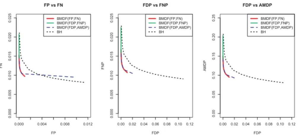
0.000 0.004 0.008 0.012 0. 000 0. 005 0. 010 0. 015 0. 020 0. 025 FP vs FN FP FN BMDF(FP,FN) BMDF(FDP,FNP) BMDF(FDP,AMDP) BH 0.00 0.02 0.04 0.06 0.08 0.10 0.12 0. 000 0. 005 0. 010 0. 015 0. 020 0. 025 FDP vs FNP FDP FN P BMDF(FP,FN) BMDF(FDP,FNP) BMDF(FDP,AMDP) BH 0.00 0.02 0.04 0.06 0.08 0.10 0.12 0. 00 0. 05 0. 10 0. 15 0. 20 0. 25 FDP vs AMDP FDP A MDP BMDF(FP,FN) BMDF(FDP,FNP) BMDF(FDP,AMDP) BH
Fig 2. Graphs of (F Pˆ ,F Nˆ ), (F DPˆ ,F N Pˆ ), and (F DPˆ ,AM DPˆ ) for three BMDFs with dif-ferent loss functions when the cost ratio varies and the BH procedure when the FDR threshold varies in a two-group composite hypothesis problem with independent Gaussian observations. Correct prior parameters are specified.
form ∈ M0, µm1 =µm2 iid∼ N(νm, k0σ2m), σ−m2 ∼Gamma(α, β). True
param-eters used to generate the data are M = 500, π = 0.1, k0 = 200, α = 4, β =
4, νm= 20.We performed 1000 simulations each with correct prior parameters and misspecified prior parameters:π∗= 0.05, k∗
0= 100, α∗= 20 and with other
parametersempirically estimated via νm =xm, β =S2
p(xm)(α−1)/(k0+ 1)), where S2 p(xm) = 1 M M X m=1 (n1−1)S2(xm1, . . . , xmn1) + (n2−1)S 2(ym 1, . . . , ymn2) (n1+n2)
is the average of pooled variances. In order to stabilize the results when π is small, we used the adjusted version of MDP, the AMDP given by L(a,θ) =
(1−a)Tθ
(θT1)+1. We implemented the three BMDFs associated with different loss
func-tions with 10 different cost ratiosC0/C1and the BH procedure with 10 different
FDR thresholds. Figure2and Figure3show graphs of three empirical risk pairs for all four procedures with correctly specified prior parameters and partially misspecified and partially empirically-estimated prior parameters, respectively. In Figure 2 with the correct prior specification, the empirical risk curves for all three BMDFs are well below that for the BH procedure indicating better performance, except for the BMDF associated with the (FDP, AMDP) pair of loss functions where the average FP loss is surprisingly high. This is because with small prior probabilityπfor the alternatives, the AMDP could be large for some simulated data, and when the cost ratioC0/C1 is very small, the BMDF
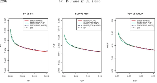
would rather sacrifice a large number of false positives to achieve the optimal combined risk of FDP and AMDP. In Figure 3, when the prior parameters are partially misspecified and partially empirically estimated, the results of all four
0.000 0.005 0.010 0.015 0. 000 0. 002 0. 004 0. 006 0. 008 0. 010 FP vs FN FP FN BMDF(FP,FN) BMDF(FDP,FNP) BMDF(FDP,AMDP) BH 0.00 0.05 0.10 0.15 0. 000 0. 002 0. 004 0. 006 0. 008 0. 010 0. 012 FDP vs FNP FDP FN P BMDF(FP,FN) BMDF(FDP,FNP) BMDF(FDP,AMDP) BH 0.00 0.05 0.10 0.15 0. 00 0. 05 0. 10 0. 15 0. 20 FDP vs AMDP FDP A MDP BMDF(FP,FN) BMDF(FDP,FNP) BMDF(FDP,AMDP) BH
Fig 3. Graphs of (F Pˆ ,F Nˆ ), (F DPˆ ,F N Pˆ ), and (F DPˆ ,AM DPˆ ) for three BMDFs with dif-ferent loss functions when the cost ratio varies and the BH procedure when the FDR threshold varies in a two-group composite hypothesis problem with independent Gaussian observations. The prior parameters are partially misspecified and partially empirically estimated.
procedures almost coincide. The simulation results lend empirical support to the theoretical result in [3] that the BH procedure has the asymptotic optimality under the loss function pair (FP, FN) as a function of the cost ratio. However, more studies regarding more general loss functions and the empirical Bayes ideas are needed to obtain more reliable conclusions.
7.4. A microarray data analysis
In a colon cancer tumor metastasis study conducted in the laboratory of Dr. Marge Pe˜na at the University of South Carolina, expression levels for 41268 genes from mice tissues were obtained through an Agilent Technology microar-ray. For each gene, five replicates were obtained for a control group and five replicates for a metastatic group. Computationally, the BMDF associated with (FP, FN) and (FDP, FNP) loss functions have relatively low cost, but the one associated with the (FDP, AMDP) loss function needs a much longer time, because it requires the computation of a posterior expectation involving all the genes. Therefore for illustration purposes, we simply randomly selected 500 genes out of the 41268 on which to apply our BMDF. We assumed the indepen-dent two-group Gaussian model, and used the partially empirically-estimated prior parameters described in Section7.3. Cost ratios used for (FP, FN), (FDP, FNP) and (FDP, AMDP) loss function pairs are, respectively,C0/C1= 3,0.2,2,
and for BH procedure the FDR threshold is 0.05. These cost ratios and thresh-olds were chosen according to the simulation results in Section7.3 in order for the four procedures to have similar empirical FDPs. Out of the 500 genes, the BMDF associated with the loss function pairs (FP, FN), (FDP, FNP), and (FDP, AMDP) found 15, 14, and 14 genes differentially expressed across groups,
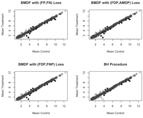
re-2 4 6 8 10 12 2 4 6 8 12 BMDF with (FP,FN) Loss Mean Control Mean Treatment 2 4 6 8 10 12 2 4 6 8 12
BMDF with (FDP,AMDP) Loss
Mean Control Mean Treatment 2 4 6 8 10 12 2 4 6 8 12 BMDF with (FDP,FNP) Loss Mean Control Mean Treatment 2 4 6 8 10 12 2 4 6 8 12 BH Procedure Mean Control Mean Treatment
Fig 4. Mean expression level of the control group versus the treatment group for 500 genes in a microarray data set. Gray circles are non discoveries and black circles are discoveries. Top left: BMDF with (FP, FN) loss function pair; top right: BMDF with (FDP, AMDP) loss function pair; bottom left: BMDF with (FDP,FNP) loss function pair; bottom right: BH procedure.
spectively, and the BH procedure found 10. Figure4shows the mean expression level of the control group versus the treatment group of the discovered genes. Notice that all 10 genes discovered by the BH procedure were also discovered by the three BMDFs.
8. Concluding remarks
BMDF developed in this paper generates a class of multiple decision procedures which are optimal in the Bayesian framework for a general class of loss functions. The results in Theorem1describe the form of the BMDF and provide an efficient algorithm of finding the associated decisions in multiple testing settings. Notice that the pairs of loss functions are not limited to those described in Section4. For example, the adjusted MDP given in Table1may help stabilize the computation of the the Bayes optimal actions when the prior probabilities of the alternative hypotheses, the πm=P r(θm = 1), π = 1,2, . . . , M,are small. Also notice that
the choice of the loss function pairs and the cost ratio should be pre-determined in consultation with specialists of the scientific discipline relevant to the specific application.
The frailty-based model is a class of flexible models for dependent data struc-ture, where the distribution of the frailty can be specified in a hierarchical manner with hyperparameters. Similarly, the prior distribution could also be dependent with frailty-based structures. Furthermore, the SMC could be easily implemented in the computations of the posterior expectations. Note, however, that not all dependent structures are frailty-based. Therefore, in real data anal-ysis, model validation is needed to see the validity of the imposed dependent structures.
One possible extension of this research is in two-class prediction problems where the form of the BMDF could be extended with the loss functions replaced by prediction errors. Besides the usual prediction loss function pair of (FP, FN) that has been studied extensively, such as in [3], we can also consider a similar class of loss functions in multiple prediction problems, where the class memberships of many new items are to be predicted simultaneously. Future studies may also include extensions to model selection, and the empirical Bayes approach to determining prior hyperparameter values. In particular, of interest is to study whether the empirical Bayes procedures are equivalent to the non-Bayesian BH multiple decision function and the procedure in [18].
Acknowledgments
The authors thank Dr. Marge Pe˜na for providing the microarray data set and for discussions regarding microarrays. They also thank the referees, associate editor, and editor for their constructive comments and criticisms which led to considerable improvements in the paper.
The authors acknowledge supports from National Science Foundation (NSF) Grants DMS 0805809 and DMS 1106435, National Institutes of Health (NIH) Grants RR17698 and R01CA154731, and Environmental Protection Agency (EPA) Grant RD-83241902-0 to the University of Arizona with subaward num-ber Y481344 to the University of South Carolina.
This paper is based on a portion of the first author’s PhD dissertation at the Department of Statistics, University of South Carolina, Columbia.
References
[1] Benjamini, Y. and Hochberg, Y.(1995). Controlling the false discovery rate: a practical and powerful approach to multiple testing.J. Roy. Statist. Soc. Ser. B 57, 1, 289–300.MR1325392 (96d:62143)
[2] Berger, J. O. (1985). Statistical decision theory and Bayesian analy-sis, Second ed. Springer Series in Statistics. Springer-Verlag, New York.
[3] Bogdan, M., Chakrabarti, A., Frommlet, F., and Ghosh, J. K. (2011). Asymptotic Bayes-optimality under sparsity of some multiple test-ing procedures. Ann. Statist.39, 3, 1551–1579. http://dx.doi.org/10. 1214/10-AOS869.MR2850212 (2012j:62019)
[4] Bogdan, M.,Ghosh, J. K.,and Tokdar, S. T.(2008). A comparison of the Benjamini-Hochberg procedure with some Bayesian rules for multiple testing. InBeyond parametrics in interdisciplinary research: Festschrift in honor of Professor Pranab K. Sen. Inst. Math. Stat. Collect., Vol.1. Inst. Math. Statist., Beachwood, OH, 211–230. http://dx.doi.org/10.1214/ 193940307000000158.MR2462208 (2009m:62018)
[5] Casella, G. and Berger, R. L. (2001). Statistical Inference, 2nd ed. Duxbury Press.
[6] Efron, B.(2008). Microarrays, empirical Bayes and the two-groups model. Statist. Sci.23, 1, 1–22.MR2431866
[7] Efron, B. (2010a). Large-scale inference. Institute of Mathematical Statistics Monographs, Vol. 1. Cambridge University Press, Cambridge.
MR2724758
[8] Efron, B. (2010b). The Future of Indirect Evidence. Statistical Sci-ence 25, 2, 145–157.
[9] Gordon, N. J. and Smith, A. F. M.(1993). Approximate non-Gaussian Bayesian estimation and modal consistency. J. Roy. Statist. Soc. Ser. B 55, 4, 913–918.MR1229888 (94b:62077)
[10] Hastie, T.,Tibshirani, R.,and Friedman, J.(2009).The elements of statistical learning, Second ed. Springer Series in Statistics. Springer, New York.MR2722294
[11] Hougaard, P. (2000). Analysis of multivariate survival data. Statistics for Biology and Health. Springer-Verlag, New York. http://dx.doi.org/ 10.1007/978-1-4612-1304-8.MR1777022 (2001h:62003)
[12] Knuth, D. E. (1973). The art of computer programming. Volume 3. Addison-Wesley Publishing Co., Reading, Mass.-London-Don Mills, Ont.
MR0445948 (56 #4281)
[13] Liu, J. S.(2001). Monte Carlo strategies in scientific computing. Springer Series in Statistics. Springer-Verlag, New York.MR1842342 (2002i:65006)
[14] M¨uller, P.,Parmigiani, G.,and Rice, K.(2007). FDR and Bayesian multiple comparisons rules. In Bayesian statistics 8. Oxford Sci. Publ. Oxford Univ. Press, Oxford, 349–370.MR2433200
[15] M¨uller, P., Parmigiani, G., Robert, C.,and Rousseau, J. (2004). Optimal sample size for multiple testing: the case of gene expression mi-croarrays. J. Amer. Statist. Assoc.99, 468, 990–1001.MR2109489
[16] Nelsen, R. B.(1999).An introduction to copulas. Lecture Notes in Statis-tics, Vol.139. Springer-Verlag, New York.MR1653203 (99i:60028)
[17] Neutial, P. and Roquain, E. On false discovery rate thresholding for classification under sparsity. To appear in Ann. Statist..
[18] Pe˜na, E. A.,Habiger, J.,and Wu, W.(2011). Power-enhanced multiple decision functions controlling family-wise error and false discovery rates. Annals of Statistics 39, 1, 556–583.
[19] Ripley, B. D. (1987). Stochastic simulation. Wiley Series in Probabil-ity and Mathematical Statistics: Applied ProbabilProbabil-ity and Statistics. John Wiley & Sons Inc., New York.MR875224 (88b:68181)
[20] Sarkar, S. K.,Zhou, T.,and Ghosh, D.(2008). A general decision the-oretic formulation of procedures controlling FDR and FNR from a Bayesian perspective. Statist. Sinica 18, 3, 925–945.MR2440399
[21] Scott, J. G. and Berger, J. O.(2006). An exploration of aspects of Bayesian multiple testing. J. Statist. Plann. Inference 136, 7, 2144–2162. http://dx.doi.org/10.1016/j.jspi.2005.08.031.MR2235051
[22] Storey, J.(2003). The positive false discovery rate: a Bayesian interpre-tation and the q-value. The Annals of Statistics 31, 2012 – 2035.
[23] Sun, W. and Cai, T. T.(2007). Oracle and adaptive compound decision rules for false discovery rate control.J. Amer. Statist. Assoc.102, 479, 901– 912. http://dx.doi.org/10.1198/016214507000000545.MR2411657