Gene expression
Scater: pre-processing, quality control,
normalization and visualization of single-cell
RNA-seq data in R
Davis J. McCarthy
1,2,3,*, Kieran R. Campbell
2,4, Aaron T. L. Lun
5and
Quin F. Wills
2,61
European Molecular Biology Laboratory, European Bioinformatics Institute, Wellcome Genome Campus, CB10 1SD
Hinxton, Cambridge, UK,
2Wellcome Trust Centre for Human Genetics, University of Oxford, Oxford OX3 7BN, UK,
3
St Vincent’s Institute of Medical Research, Fitzroy, Victoria 3065, Australia,
4Department of Physiology, Anatomy
and Genetics, University of Oxford, Oxford OX1 3QX, UK,
5CRUK Cambridge Institute, University of Cambridge,
Cambridge CB2 0RE, UK and
6Weatherall Institute for Molecular Medicine, University of Oxford, John Radcliffe
Hospital, Oxford OX3 9DS, UK
*To whom correspondence should be addressed. Associate Editor: Ivo Hofacker
Received on August 15, 2016; revised on November 7, 2016; editorial decision on December 1, 2016; accepted on December 7, 2016
Abstract
Motivation:
Single-cell RNA sequencing (scRNA-seq) is increasingly used to study gene expression
at the level of individual cells. However, preparing raw sequence data for further analysis is not a
straightforward process. Biases, artifacts and other sources of unwanted variation are present in
the data, requiring substantial time and effort to be spent on pre-processing, quality control (QC)
and normalization.
Results:
We have developed the R/Bioconductor package
scater
to facilitate rigorous pre-processing,
quality control, normalization and visualization of scRNA-seq data. The package provides a
conveni-ent, flexible workflow to process raw sequencing reads into a high-quality expression dataset ready
for downstream analysis.
scater
provides a rich suite of plotting tools for single-cell data and a
flex-ible data structure that is compatflex-ible with existing tools and can be used as infrastructure for future
software development.
Availability and Implementation:
The open-source code, along with installation instructions,
vi-gnettes and case studies, is available through Bioconductor at http://bioconductor.org/packages/
scater.
Contact:
[email protected]
Supplementary information:
Supplementary data
are available at
Bioinformatics
online.
1 Introduction
Single-cell RNA sequencing (scRNA-seq) describes a broad class of techniques which profile the transcriptomes of individual cells. This provides insights into cellular processes at a resolution that cannot be matched by bulk RNA-seq experiments (Hebenstreit and Teichmann, 2011;Shaleket al., 2013). With scRNA-seq data, the contributions of different cell types to the expression profile of a
heterogeneous population can be explicitly determined. Rare cell types can be interrogated and new cell subpopulations can be dis-covered. Graduated processes such as development and differenti-ation can also be studied in greater detail. However, this improvement in resolution comes at the cost of increased technical noise and biases. This means that pre-processing, quality control and normalization are critical to a rigorous analysis of scRNA-seq
VCThe Author 2017. Published by Oxford University Press. 1179
This is an Open Access article distributed under the terms of the Creative Commons Attribution License (http://creativecommons.org/licenses/by/4.0/), which permits unrestricted reuse, distribution, and reproduction in any medium, provided the original work is properly cited.
doi: 10.1093/bioinformatics/btw777 Advance Access Publication Date: 14 January 2017 Original Paper
data. The increased complexity of the data across hundreds or thou-sands of cells also requires sophisticated visualization tools to assist interpretation of the results.
Numerous statistical methods and software tools have been pub-lished for scRNA-seq data (Angereret al., 2015;Finaket al., 2015;
Guo et al., 2015; Julia et al., 2015; Kharchenko et al., 2014;
Trapnellet al., 2014). However, all of these assume that quality con-trol and normalization have already been applied. Fewer methods are available in the literature to perform these basic steps in scRNA-seq data processing (Ilicicet al., 2016). This issue is exacerbated by the diversity of scRNA-seq datasets with respect to the experimental protocol and the biological context of the study, meaning that a sin-gle processing pipeline with fixed parameters is unlikely to be uni-versally applicable. Rather, software tools are required that support an interactive approach to analysis. This allows parameters to be fine-tuned for the study at hand in response to any issues diagnosed during data exploration. The provided functionality should also pro-cess the data in a statistically rigorous manner and encourage repro-ducible bioinformatics analyses.
One of the most widely used frameworks for interactive analysis is the R programming language, extended for biological data ana-lysis through the Bioconductor project (Huberet al., 2015). While Bioconductor packages have been widely used for bulk RNA-seq data, the existing data structures (like the ExpressionSet class) are not sufficient for scRNA-seq data. This is because they do not sup-port data types that are specific to single-cell studies, e.g. cell–cell distance matrices for clustering. For larger studies, this also includes data beyond expression profiles such as intensity values from fluorescence-activated cell sorting, cell imaging data and informa-tion from epigenetic and targeted genotyping assays. Existing meth-ods for processing and applying quality control to scRNA-seq data are similarly inadequate. In particular, current visualization methods designed for exploratory data analysis of bulk transcriptomic experi-ments are unsuited to datasets containing hundreds or thousands of cells. The large size of each dataset also favours methods such as kal-listo(Brayet al., 2016) andSalmon(Patroet al., 2016) for rapidly quantifying gene expression, but support for the output of these methods is currently limited. Extensions to the current computa-tional infrastructure are required to provide appropriate data struc-tures and methods that can accommodate these rich scRNA-seq datasets for integrative analyses of expression and other assay data along with the accompanying metadata.
Here we presentscater, an open-source R/Bioconductor software package that implements a convenient data structure for representing scRNA-seq data and contains functions for pre-processing, quality control, normalization and visualization. The package provides wrap-per functions for runningkallistoandSalmonon raw read data and converting their output into gene-level expression values, methods for computing and visualizing quality-control metrics for cells and genes, and methods for normalization and correction of uninteresting cova-riates. This is done in a single software environment which enables seamless integration with a large number of existing tools for scRNA-seq data analysis in R. Thescaterpackage provides basic infrastruc-ture upon which customized scRNA-seq analyses can be constructed, and we anticipate the package to be useful across the whole spectrum of users, from experimentalists to computational scientists.
2 Methods, data and implementation
2.1 Case study with scRNA-seq data
The results presented in the main paper and supplementary case study use an unpublished single-cell RNA-seq dataset consisting of
73 cells from two lymphoblast cell lines of two unrelated individ-uals. Cells were captured, lysed and cDNA generated using the popular C1 platform from Fluidigm, Inc. (https://www.fluidigm. com/products/c1-system). The processing of the two cell lines was replicated across two machines, with the nuclei of the two cell lines stained with different dyes before mixing on each machine. Cells were imaged before lysis, with an example image provided together with these data (see Case Study in Supplementary Material). Samples were sequenced with paired-end sequencing using the HiSeq 2500 Sequencing system (Illumina). RNA-seq reads were mapped to a custom genome reference, consisting of Homo sapiens GRCh37 (primary assembly from ftp://ftp.ensembl.org/pub/release-75/fasta/homo_sapiens/dna/, last accessed 14.08.2015), Epstein-Barr Virus type 1 (B95-8 strain, Accession NC_007605.1) and ERCC RNA spike-ins (ThermoFisher). Reads in fastq format were aligned with TopHat2 v2.0.12 (Kimet al., 2013), using Bowtie2 v2. 2.3.0 (Langmead and Salzberg, 2012) as the core mapping engine (– mate-inner-dist 190 –mate-std-dev 40 –report-secondary-align-ments) and other default parameters. Potential PCR duplicates were marked with Picard MarkDuplicates v1.92(1464). Reads mapping uniquely to annotated exon features were counted using htseq-count implemented in HTSeq, version 0.6.1p1 (Anderset al., 2015).
Further case studies usingscateron published data, for example from 3000 mouse cortex cells (Zeiselet al., 2015) and 1200 cells from early-development mouse embryos (Scialdoneet al., 2016) are available at http://dx.doi.org/10.5281/zenodo.59897. All materials required to reproduce the results presented in this paper are avail-able at http://dx.doi.org/10.5281/zenodo.60139.
2.2 Implementation
Thescaterpackage is an open-source R package available through Bioconductor. Key aspects of the code are written in Cþþto mini-mize computational time and memory use, and the package scales well to large datasets. For example, consider the Macoskoet al. (2015)dataset, which contains more than 44 000 cells. The core sca-ter functions to create an SCESet object and calculate QC metrics took approximately two minutes to complete on an early 2015 MacBook Pro laptop with 2.9 GHz Intel Core i5 processor and 16 Gb of RAM. Subsetting the SCESet object takes only a few se-conds, and producing a PCA plot with the plotPCA function takes less than a minute.
The package builds on many other R packages, including
Biobase and BiocGenerics for core Bioconductor functionality (Huberet al., 2015); destiny(Angereret al., 2015) andRtsnefor dimensionality reduction; andedgeR (Robinsonet al., 2010) and
limma(Ritchieet al., 2015) for model fitting and statistical analyses. The plotting functionality in the package usesggplot2. A full set of dependencies is provided in theSupplementary Materials.
3 Results
3.1 The
scater
package
Thescaterpackage offers a workflow to convert raw read sequences into a dataset ready for higher-level analysis within the R program-ming environment (Fig. 1). In addition,scaterprovides basic compu-tational infrastructure to standardize and streamline scRNA-seq data analyses. Key features ofscaterinclude: (i) the ‘single-cell ex-pression set’ (SCESet) class, a data structure specialized for scRNA-seq data; (ii) wrapper methods to runkallistoandSalmonand pro-cess their output into gene-level expression values; (iii) automated calculation of quality control metrics, with QC visualization and
filtering methods to retain high-quality cells and informative fea-tures; (iv) extensive visualization capabilities for inspection of scRNA-seq data and (v) methods to identify and remove uninterest-ing covariates affectuninterest-ing expression across cells. The package inte-grates many commonly used tools for scRNA-seq data analysis and provides a foundation on which future methods can be built. The methods inscaterare agnostic to the form of the input data and are compatible with counts, transcripts-per-million, counts-per-million, FPKM or any other appropriate transformation of the expression values.
3.2 SCESet: a data structure for single-cell expression
data
Thescaterpackage is built around the SCESet class (Supplementary Fig. S1) which provides a sophisticated container for scRNA-seq data. This class inherits from the ExpressionSet class in Bioconductor’sBiobasepackage (Huberet al., 2015), which allows assay data (and multiple transformations thereof), gene or transcript metadata and sample metadata to be combined in a single object to empower robust analyses. While the ExpressionSet class is the basis of many microarray and bulk RNA-seq analysis methods in Bioconductor, extensions to the class design are necessary to support scRNA-seq data analyses. Specifically, the SCESet class adds slots to store a reduced-dimension representation of the expression profiles, to easily visualize the relationships between cells; cell–cell and gene– gene pairwise distance matrices, for clustering or regulatory network reconstruction; bootstrapped expression results (such as from kal-listo), to gauge the accuracy of expression quantification; consensus clustering results, where cluster assignments for each cell are com-bined from different methods to improve reliability; information about feature controls (such as ERCC spike-ins), which is required in downstream steps such as normalization, QC and detection of highly variable genes; and several more (Supplementary Fig. S1). With these extra slots, SCESet objects can support analyses of scRNA-seq data that ExpressionSet cannot. In addition, extra data types such as FACS marker expression or epigenetic information can be easily stored in each SCESet object for integration with the single-cell expression profiles.
An SCESet data object can be easily subsetted by row or column to remove unwanted genes or cells, respectively, from all data and metadata fields stored in the object. Furthermore, data and meta-data in multiple SCESet objects can be easily combined e.g. to in-corporate cells from different experimental batches. SCESet objects can also be converted to other R data structures, or saved to disk in structured, shareable formats. Further details on the class, including its motivation and execution, are available in the Supplementary Case Study and the package documentation. All methods available inscaterare applicable to instances of the SCESet class and exploit the availability and richness of (meta)data stored in each SCESet object.
3.3 Data pre-processing
An important initial step in scRNA-seq data processing is to quan-tify the expression level of genomic features such as transcripts or genes from the raw sequencing data. Approaches to expression quantification from raw reads are, in principle, the same for scRNA-seq as they are for bulk RNA-scRNA-seq (Kanitzet al., 2015;Tenget al., 2016). Read counts obtained from conventional quantification methods such as HTSeq(Anders et al., 2015) andfeatureCounts
(Liaoet al., 2014) can be readily stored in an SCESet object and used in a scater workflow (Fig. 1). Another option is to use
computationally efficient pseudoalignment methods such askallisto
andSalmon. This is especially appealing for large scRNA-seq data-sets containing hundreds to tens of thousands of cells. To this end,
scateralso provides wrapper functions forkallistoandSalmonso that fast quantification of transcript-level expression can be man-aged completely within an R programming environment. A common subsequent step for these methods is to collapse transcript-level ex-pression to gene-level exex-pression. Exploiting the biomaRt R/ Bioconductor package, scater provides a convenient function for using Ensembl annotations (Yateset al., 2016) to obtain gene-level expression values and gene or transcript annotations.
3.4 Data quality control
Thescaterpackage provides methods to compute relevant QC met-rics for an SCESet object. Given a set of control genes and/or cells, a variety of QC metrics will be computed and returned to the object in a single call to the calculateQCMetrics function (see package docu-mentation). Cell-specific QC metrics include the total count across all genes, the total number of expressed genes, and the percentage of counts allocated to control genes like spike-in transcripts or mito-chondrial genes. These metrics are useful for identifying low-quality cells—for example, a high percentage of counts mapping to spike-ins typically indicates that a small amount of RNA was captured for the cell, suggesting protocol failure or death of the cell in processing that renders it unsuitable for downstream analyses. For each gene, QC metrics such as the average expression level and the proportion of cells in which the gene is expressed are computed. This can be used to identify low-abundance genes or genes with high dropout rates that should be filtered out prior to downstream analyses. All of
Fig. 1.An overview of thescaterworkflow, from raw sequenced reads to a high quality dataset ready for higher-level downstream analysis. For step 5, explanatory variables include experimental covariates like batch, cell source and other recorded information, as well as QC metrics computed from the data. Step 6 describes an optional round of normalization to remove effects of particular explanatory variables from the data. Automated computation of QC metrics and extensive plotting functionality support the workflow
these metrics are used by scater to construct QC plots to diagnose potential issues with data quality. This facilitates quality control which—despite attempts at automation (Ilicicet al., 2016)—still re-quires manual intervention to account for aspects of the data specific to each study. The package documentation provides full details of the QC metrics produced.
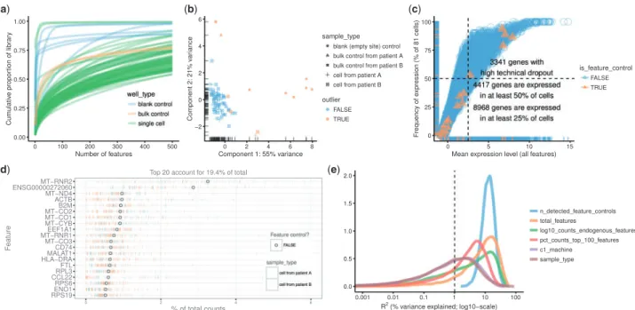
Inscater, the default plot method for an SCESet object produces a cumulative expression plot (Fig. 2a). This plot describes how reads are distributed across genes, distinguishing between low-complexity libraries (where very few genes contain most of the counts) and their high-complexity counterparts (where counts are distributed more evenly across genes). For example, there is substantial variability in library complexity among cells in the case study dataset in
Figure 2a. Some cells have profiles similar to the blank wells, sug-gesting that library preparation or sequencing failed for these cells and that the corresponding libraries should be removed prior to fur-ther analysis. Cell phenotype variables can be incorporated into these plots to highlight differences in expression distributions for different types of cells. For example, the curve for each cell is col-oured by the type of well that produced the library (Fig. 2a), while cells can also be split into separate facets by library type to show more metadata variables simultaneously (see Supplementary Case Study). Cumulative expression plots should be favoured over box-plots as the default method for visualizing expression distributions across cells in a dataset, as the latter performs poorly at handling the long tail of low- and zero-expression observations in scRNA-seq data.
The plotPCA function implements an approach to automatic outlier detection using multivariate normal methods applied to the cell-level QC metrics (Ilicicet al., 2016). It produces a PCA plot computed from QC metrics, where cells corresponding to detected
outliers are marked (Fig. 2b). Briefly, semi-robust principal compo-nents are computed from robustly sphered QC metrics data, using the pcout function from themvoutlierR package (Filzmoseret al., 2008). These components are used to calculate distances for each cell, which are then used to compute weights for outlier detection. By default, the following QC metrics are used in this procedure: the percentage of counts from the top 100 features, the total number of features with detectable expression, the percentage of counts from control features, the number of detected feature controls, the log-scaled counts from endogenous features and log-transformed counts from feature controls. The user can specify QC metrics or other cell metadata variables to use for outlier detection with the ‘selected_variables’ argument to plotPCA. Detected outliers corres-pond to low-quality cells with abnormal library characteristics (e.g. low total counts and few expressed genes) that should be removed prior to downstream analysis. This automated approach is powerful but also somewhat opaque with respect to how outliers are defined, and so complements simpler filtering approaches that apply thresh-olds to particular QC metrics.
The plotQC function generates many types of plots useful for quality control, such as a plot to visualize the frequency of expres-sion of features against their average expresexpres-sion level (Fig. 2c). Such plots are useful because scRNA-seq data are characterized by a high frequency of ‘dropout’ events, i.e. no observed expression (such as no read counts) in a particular cell for a gene that is actually pressed in that cell. Indeed, most genes will not have detectable ex-pression in every cell. With plotQC, control features that should be present in each cell can be highlighted easily in the plot, allowing technical dropouts to be distinguished from biological heterogeneity of expression. Typical scRNA-seq datasets will show a broadly sig-moidal relationship between average expression level and frequency
(a) (b)
(d) (e)
(c)
Fig. 2.Different types of QC plots that can be generated withscater. (a) Cumulative expression plot showing the proportion of the library accounted for by the top 1–500 most highly expressed features. (b) PCA plot produced using a subset of the QC metrics computed withscater’scalculateQCMetrics function. (c) Plot of fre-quency of expression (percentage of cells in which the feature is deemed expressed) against mean expression level across cells. The vertical dotted line shows the median of the gene mean expression levels, and the horizontal dotted line indicates 50% frequency of expression. (d) Plot of the 20 most highly expressed fea-tures (computed according to the highest total read counts) across all cells in the dataset. For each feature, the circle represents the percentage of counts across all cells that correspond to that feature. The features are ordered by this value. The bars for each feature show the percentage of counts corresponding to the fea-ture in each individual cell, providing a visualization of the distribution across cells. (e) Density plot showing the percentage of variance explained by a set of ex-planatory variables across all genes. Each individual plot is produced by a single call with either the function plot (a), plotPCA (b) or plotQC (c–e)
of expression across cells. This is consistent with expected behaviour where genes with greater average expression are more readily cap-tured during library preparation and are detected at a greater fre-quency (Brennecke et al., 2013; Kimet al., 2015;Vallejos et al., 2015).
With plotQC, we can also produce a plot to visualize the most highly expressed features in the dataset (Fig. 2d). This provides a feature-centric overview of the dataset that visualizes the features with highest total expression across all cells, while also displaying the distribution of cell-level expression values for these features. It is common to see ERCC spike-ins (if used), mitochondrial and riboso-mal genes among the highest expressed genes, while datasets consist-ing of healthy cells will also show high levels of constitutively expressed genes likeACTB. This plot allows the analyst to quickly check that the gene- or transcript-level quantification is behaving as expected, and to flag datasets where it is not.
Another important step in quality control is to identify variables (experimental factors or computed QC metrics) that drive variation in expression data across cells. The plotQC function provides a novel approach to identifying variables that have substantial ex-planatory power for many genes. For each variable in the phenoData slot of the SCESet object, we fit a linear model for each feature with only that variable as the explanatory variable. We then plot the distribution of the marginalR2values across all features for the variables with the most explanatory power for the dataset (Fig. 2e). The variables are ranked by medianR2across features in the
plot, allowing users to identify variables that may need to be con-sidered during normalization or statistical modelling. The plotQC function can also assess the influence of variables of interest by plot-ting principal components of the expression matrix most strongly correlated with a variable of interest against that variable. For ex-ample, in the Case Study data, the first principal component is corre-lated with the C1 machine used to process the cell (Supplementary Fig. S2).
We also introduce the plotPhenoData function for convenient plotting of cell phenotype information (including QC metrics), and the plotFeatureData function for plotting feature information (see examples in the Supplementary Case Study). These methods will work not only on the SCESet class defined inscater, but also on any ExpressionSet object, providing sophisticated plotting functionality for many other Bioconductor packages and contexts.
Thescatergraphical user interface (GUI) provides convenient ac-cess toscater’s QC and visualization methods (Supplementary Figs S4–S6). This opens an interactive interface in a web browser that fa-cilitates exploration of the data through QC plots and other intuitive visualizations. The GUI allows users of any background to easily examine the effects of changing multiple parameters, which can be helpful for quickly conducting exploratory data analysis. Useful set-tings can then be stored in R scripts to ensure that data analyses are reproducible.
In summary,scaterprovides a variety of novel and convenient methods to visualize an scRNA-seq dataset for QC. Low-quality cells and uninteresting genes can then be easily removed by filtering and subsetting the SCESet data structure prior to further analysis.
3.5 Data visualization
Dimensionality reduction techniques are necessary to convert high-dimensional expression data into low-high-dimensional representations for intuitive visualization of the relationships, similarities and differ-ences between cells. To this end,scaterprovides convenient func-tions to apply a variety of dimensionality reduction procedures to
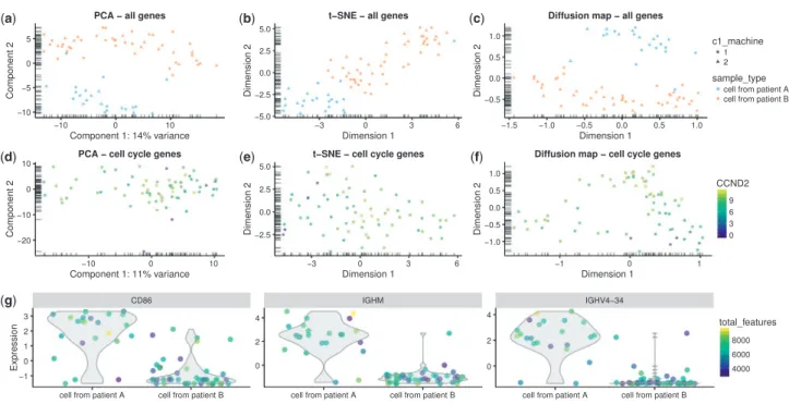
the cells in an SCESet object. Functions include plotPCA, to perform a principal components analysis; plotTSNE, to perform t-distributed stochastic neighbour embedding (Van der Maaten and Hinton, 2008), which has been widely used for scRNA-seq data (Amiret al., 2013; Bendall et al., 2014; Macosko et al., 2015); plotDiffusionMap, to generate a diffusion map (Haghverdiet al., 2015) for visualizing differentiation processes; and plotMDS, to generate multi-dimensional scaling plots (Fig. 3a–c). The plotReducedDim function can also be used to plot any reduced-dimension representation of cells (e.g. an independent component analysis produced bymonocle(Trapnellet al., 2013) or similar) that is stored in an SCESet object.
By default, the PCA and t-SNE plots are produced using the fea-tures with the most variable expression across all cells. We focus on the most variable genes to highlight any heterogeneity in the data that might be driving interesting differences between cells. Alternatively, we can applya priori knowledge to define a set of genes that are associated with a biological process of interest, and construct plots using only these features. For example,Scialdone et al.(2015)found that using prior knowledge to define feature sets is vital for exploring processes like the cell cycle, which can have substantial effects on single-cell expression measurements (Buettner et al., 2015). The subsetting and filtering methods for SCESet ob-jects facilitate the generation of reduced-dimension plots for particu-lar gene sets, in order to investigate certain effects in the data such as those due to the cell cycle (Fig. 3d–f).
The various types of reduced-dimension plots can be used to examine the structure of the cell population, including the formation of distinct subpopulations or the presence of continuous trajectories. Cell-level variables stored in the SCESet object can be used to define the shape, colour and size of points plotted, allowing more informa-tion to be conveniently incorporated into each plot (e.g. cells are col-oured by CCND2 expression in Fig. 3d–f). The plotExpression function is also provided for plotting expression levels of a particu-lar gene against any of the cell phenotype variables or the expression level of another feature (Fig. 3g). This allows the user to inspect the expression levels of a feature or set of features in full detail, rather than relying only on summary information and reduced-dimension plots where information is necessarily lost.
3.6 Data normalization and batch correction
Scaling normalization is typically required in RNA-seq data analysis to remove biases caused by differences in sequencing depth, capture efficiency or composition effects between samples. Frequently used methods for scaling normalization include the trimmed mean of M-values (Robinson and Oshlack, 2010), relative log-expression (Anders and Huber, 2010) and upper-quartile methods (Bullard et al., 2010), all of which are available for use inscater. In addition,
scateris tightly integrated with the scran package, which imple-ments a method utilizing cell pooling and deconvolution to compute size factors better suited to scRNA-seq data (Lunet al., 2016b).Lun et al.(2016a) also offers further discussion of the respective benefits and drawbacks of spike-in normalization and non-DE normalization.
After scaling normalization, further correction is typically required to ameliorate or remove batch effects. For example, in the case study dataset, cells from two patients were each processed on two C1 machines. Although C1 machine is not one of the most im-portant explanatory variables on a per-gene level (Fig. 2e), this fac-tor is correlated with the first principal component of the log-expression data (Fig. 2f). This effect cannot be removed by scaling
normalization methods, which target cell-specific biases and are not sufficient for removing large-scale batch effects that vary on a gene-by-gene basis (Fig. 4a). Here we present two possibilities, both easily implemented in a scater workflow.
The C1 machine effect is known from the design of the experi-ment, so we can easily regress out this effect inscater. With the normaliseExprs function the user can supply a design matrix of vari-ables to regress out of the expression values, and residuals from the linear model fit can be used as expression values for downstream analyses. For the dataset here, we fit a linear model to thescran
normalized log-expression values with the C1 machine as an ex-planatory factor. (We also use the log-total counts from endogenous genes, percentage of counts from the top 100 most highly expressed genes and percentage of counts from control genes as additional
covariates to control for these other unwanted technical effects.) We then use the residuals from the fitted model for further analyses (see Case Study inSupplementary Material). This approach successfully removes the C1 machine effect as a major source of variation be-tween cells; the first principal component now separates the cells from the two patients, as expected (Fig. 4b). This approach needs to be used carefully as single-cell data often deviate from normal distri-butions, but in many cases, as here, it can successfully ameliorate large-scale known batch effects.
In addition to removing known batch effects, it can be important for large datasets to identify (potentially unknown) sources of un-wanted variation (Gru¨n and van Oudenaarden, 2015;Hickset al., 2015;Leeket al., 2010).scateris compatible with existing methods such assvaseq(Leek and Storey, 2007;Leek, 2014) andRUVSeq
(a) (b) (c)
(d)
(g)
(e) (f)
Fig. 3.Reduced dimension representations of cells and gene expression plots withscater.Plots are shown using all genes (a–c) and cell cycle genes only (d–f) using PCA (a,d), t-SNE (b,e) and diffusion maps (c,f), where each point represents a cell. In the top row (a–c), points are coloured by patient of origin, sized by total features (number of genes with detectable expression) and the shape indicates the C1 machine used to process the cells. In the second row (d–f), points are col-oured by the expression ofCCND2(a gene associated with the G1/S phase transition of the cell cycle) in each cell. Furthermore, with the plotExpression function, gene expression can be plotted against any cell metadata variables or the expression of another gene—here, expression for the CD86, IGH44 and IGHV4-34 genes in each cell is plotted against the patient of origin (g). The function automatically detects whether the x-axis variable is categorical or continuous and plots the data accordingly, with x-axis values ‘jittered’ to avoid excessive overplotting of points with the same x coordinate
(a) (b) (c)
Fig. 4.Normalization and batch correction withscater. Principal component analysis plots showing cell structure in the first two PCA dimensions using various normalization methods that can be easily applied inscater, including endogenous size-factor normalization using methods from thescranpackage (a); expression residuals after applying size-factor normalization and regressing out known, unwanted sources of variation (b); and removal of one hidden factor identified using the RUVs method from theRUVpackage (c). In all plots, the colour of points is determined by the patient from which cells were obtained, shape is determined by the C1 machine used to process the cells and size reflects the total number of genes with detectable expression in the cell
(Rissoet al., 2014) to identify and remove these unwanted sources of variation. Here, just removing the first latent variable identified by the RUVs method fromRUVSeqis sufficient to remove the ma-chine effect, as the PCA plot now separates cells by patient rather than C1 machine (Fig. 4c). More targeted applications of these methods can be used to remove specific effects, for example, by identifying latent factors from cell cycle genes to remove the cell cycle effect.
We emphasize that it is generally preferable to incorporate batch effects or latent variables into statistical models used for inference. Where this is not possible (e.g. for visualization), directly regressing out these uninteresting factors is required to obtain ‘corrected’ ex-pression values for further analysis. Furthermore, a general risk of removing latent factors is that interesting biological variation may be removed along with the presumed unwanted variation. Users should therefore apply such methods with appropriate caution, par-ticularly when an analysis aims to discover biological conditions, such as new cell types.
3.7 Software and data integration
As part of the R/Bioconductor ecosystem,scatercan be easily inte-grated with other software for scRNA-seq data analysis (Supplementary Fig. S3). As the SCESet class builds on existing Bioconductor data structures, most Bioconductor packages for ex-pression analyses are able to operate seamlessly with SCESet objects. Tools that can integrate easily withscaterinclude many options for data normalization (Dinget al., 2015;Lunet al., 2016b;Vallejos et al., 2015), differential expression analysis (Finak et al., 2015;
Kharchenkoet al., 2014;Trapnellet al., 2014;Vallejoset al., 2016), heterogeneous gene expression analyses (Vallejoset al., 2015), clus-tering (Fanet al., 2016;Gru¨net al., 2015;Guoet al., 2015;Kiselev et al., 2016), latent or hidden variable analysis (Chikinaet al., 2015;
Leek, 2014;Rissoet al., 2014;Stegleet al., 2012), cell cycle phase identification (Scialdoneet al., 2015) and pseudotime computation (Angereret al., 2015;Campbell and Yau, 2016;Juliaet al., 2015;
Trapnellet al., 2014). Thescaterpackage bridges the gap between raw reads and these downstream analysis tools by providing the pre-processing, QC, visualization and normalization methods and a data structure combining multiple data modalities and metadata ne-cessary for convenient, robust and reproducible analyses of scRNA-seq data (seeSupplementary Materialfor discussion of entry points to several third party tools fromscater).
4 Discussion
Single-cell RNA sequencing is widely used for high-resolution gene expression studies investigating the behaviour of individual cells. While scRNA-seq data can provide substantial biological insights, the complexity and noise of the data is also much greater than that of conventional bulk RNA-seq. Thus, rigorous analysis of scRNA-seq data requires careful quality control to remove low-quality cells and genes, as well as normalization to adjust for biases and batch ef-fects in the expression data. Failure to carry out these procedures correctly is likely to compromise the validity of all downstream ana-lyses (Gru¨n and van Oudenaarden, 2015;Hickset al., 2015;Leek et al., 2010).
Here, we present an R/Bioconductor package,scater, that pro-vides crucial infrastructure and methods for low-level scRNA-seq data analysis. The package introduces a data structure tailored to scRNA-seq data that is compatible with a vast number of existing tools in the Bioconductor project. The scater data structure
combines multiple transformations of the expression data with cell and feature (gene or transcript) metadata and allows datasets to be easily standardized and shared. Wrapper functions for the popular RNA-seq quantification methodskallistoandSalmonfacilitate the processing of raw read sequences to a SCESet object in R with ex-pression data and accompanying metadata.
Quality control is a vital preliminary step for scRNA-seq and can be a time-consuming manual task. We present a tool for auto-mated computation of QC metrics, novel plotting methods for QC and convenient subsetting and filtering methods to substantially sim-plify the process of filtering out unwanted or problematic cells and genes. The package provides a large array of sophisticated plotting functions so that cells can be visualized with a variety of popular dimensionality-reduction techniques in plots that incorporate cell metadata and expression values as plotting variables.
Normalization is a critical aspect of scRNA-seq data processing that is supported byscater. Scaling normalization methods, includ-ing the sinclud-ingle-cell specific methods in thescranpackage, are seam-lessly integrated into ascater workflow. Methods for identifying and removing batch effects and other types of unwanted variation are supported both with internal methods and through integration with a multitude of tools available in the R/Bioconductor environ-ment. Once identified, important covariates and latent variables can be flagged for inclusion in downstream statistical models or their ef-fects regressed out of normalized expression values. The package is thoroughly documented and a recent step-by-step workflow article demonstrates detailed use ofscaterin combination with other ana-lysis packages in a range of scenarios (Lunet al., 2016a).
Future development will include further extensions to data struc-tures that will enable tight integration of single-cell transcriptomic, genetic and epigenetic data, as well as further refinement of the methods available as the single-cell field matures. Althoughscater
has been produced for scRNA-seq data, its capabilities are well suited for single-cell qPCR data and bulk RNA-seq data, and may prove useful for supporting analyses of these data types.
5 Conclusion
Thescaterpackage eases the burden for a user tasked with produc-ing a high-quality sproduc-ingle-cell expression dataset for downstream ana-lysis. The intuitive GUI implemented inscaterprovides an easy entry point into rigorous analysis of scRNA-seq data for users without a computational background, enabling them to process raw reads into high-quality expression data within a single computing environ-ment. Experienced users can take advantage ofscater’s data struc-tures, wide array of methods, suitability for scripted analyses and seamless integration with many other R/Bioconductor analysis tools. The data structures and methods inscaterprovide basic infrastruc-ture upon which new scRNA-seq analysis tools can be developed. We anticipate thatscaterwill be a useful resource for both analysts and software developers in the single-cell RNA sequencing field.
Acknowledgements
We thank Marco Salvetti for provision of the two samples and Zam Cader for processing the samples. We would also like to acknowledge Peter Donnelly and Oliver Stegle for support and helpful discussions.
Funding
This work was supported by the National Health and Medical Research Council of Australia [APP1112681 to D.J.M.], by core funding from the
European Molecular Biology Laboratory [D.J.M.], core funding from Cancer Research UK [A17197 to A.T.L.L.], the United Kingdom Medical Research Council [studentship to K.R.C.] and the Oxford Single Cell Biology Consortium [Q.F.W.].
Conflict of Interest: none declared.
References
Amir,E.A.D.et al. (2013) viSNE enables visualization of high dimensional single-cell data and reveals phenotypic heterogeneity of leukemia. Nat. Biotechnol.,31, 545–552.
Anders,S. and Huber,W. (2010) Differential expression analysis for sequence count data.Genome Biol.,11, R106.
Anders,S. et al. (2015) HTSeq–a Python framework to work with high-throughput sequencing data.Bioinformatics,31, 166–169.
Angerer,P.et al. (2015) destiny: diffusion maps for large-scale single-cell data in R.Bioinformatics,32, 1241–1243.
Bendall,S.C.et al. (2014) Single-cell trajectory detection uncovers progression and regulatory coordination in human B cell development. Cell, 157, 714–725.
Bray,N.L.et al. (2016) Near-optimal probabilistic RNA-seq quantification.
Nat. Biotechnol.,34, 525–527.
Brennecke,P.et al. (2013) Accounting for technical noise in single-cell RNA-seq experiments.Nat. Methods,10, 1093–1095.
Buettner,F.et al. (2015) Computational analysis of cell-to-cell heterogeneity in single-cell RNA-sequencing data reveals hidden subpopulations of cells.
Nat. Biotechnol.,33, 155–160.
Bullard,J.H.et al. (2010) Evaluation of statistical methods for normalization and differential expression in mRNA-Seq experiments. BMC Bioinformatics,247, 1–62.
Campbell,K. and Yau,C. (2016) Ouija: Incorporating prior knowledge in single-cell trajectory learning using Bayesian nonlinear factor analysis.
bioRxiv, 060442.
Chikina,M.et al. (2015) CellCODE: a robust latent variable approach to dif-ferential expression analysis for heterogeneous cell populations.
Bioinformatics,31, 1584–1591.
Ding,B.et al. (2015) Normalization and noise reduction for single cell RNA-seq experiments.Bioinformatics,31, 2225–2227.
Fan,J.et al. (2016) Characterizing transcriptional heterogeneity through path-way and gene set overdispersion analysis.Nat. Methods,13, 241–244. Filzmoser,P.et al. (2008) Outlier identification in high dimensions.Comput.
Stat. Data Anal.,52, 1694–1711.
Finak,G.et al. (2015) MAST: a flexible statistical framework for assessing transcriptional changes and characterizing heterogeneity in single-cell RNA sequencing data.Genome Biol.,16, 278.
Gru¨n,D. and van Oudenaarden,A. (2015) Design and analysis of single-cell sequencing experiments.Cell,163, 799–810.
Gru¨n,D.et al. (2015) Single-cell messenger RNA sequencing reveals rare intes-tinal cell types.Nature,525, 251–255.
Guo,M.et al. (2015) SINCERA: a pipeline for single-cell RNA-Seq profiling analysis.PLoS Comput. Biol.,11, e1004575.
Haghverdi,L.et al. (2015) Diffusion maps for high-dimensional single-cell analysis of differentiation data.Bioinformatics,31, 2989–2998.
Hebenstreit,D. and Teichmann,S.A. (2011) Analysis and simulation of gene expression profiles in pure and mixed cell populations. Phys. Biol., 8, 035013.
Hicks,S.C.et al. (2015) On the widespread and critical impact of systematic bias and batch effects in single-cell RNA-Seq data.bioRxiv, 025528. Huber,W.et al. (2015) Orchestrating high-throughput genomic analysis with
Bioconductor.Nat. Methods,12, 115–121.
Ilicic,T.et al. (2016) Classification of low quality cells from single-cell RNA-seq data.Genome Biol.,17, 29.
Julia,M.et al. (2015) Sincell: an R/Bioconductor package for statistical assess-ment of cell-state hierarchies from single-cell RNA-seq.Bioinformatics,31, 3380–3382.
Kanitz,A.et al. (2015) Comparative assessment of methods for the computa-tional inference of transcript isoform abundance from RNA-seq data.
Genome Biol.,16, 150.
Kharchenko,P.V.et al. (2014) Bayesian approach to single-cell differential ex-pression analysis.Nat. Methods,11, 740–742.
Kim,D.et al. (2013) TopHat2: accurate alignment of transcriptomes in the presence of insertions, deletions and gene fusions.Genome Biol.,14, R36. Kim,J.K.et al. (2015) Characterizing noise structure in single-cell RNA-seq
distinguishes genuine from technical stochastic allelic expression. Nat. Commun.,6, 8687.
Kiselev,V.Y.et al. (2016) SC3 –– consensus clustering of single-cell RNA-Seq data.bioRxiv, 036558.
Langmead,B. and Salzberg,S.L. (2012) Fast gapped-read alignment with Bowtie 2.Nat. Methods,9, 357–359.
Leek,J.T. (2014) svaseq: removing batch effects and other unwanted noise from sequencing data.Nucleic Acids Res.,42, e161.
Leek,J.T. and Storey,J.D. (2007) Capturing heterogeneity in gene expression studies by surrogate variable analysis.PLoS Genet.,3, 1724–1735. Leek,J.T.et al. (2010) Tackling the widespread and critical impact of batch
ef-fects in high-throughput data.Nat. Rev. Genet.,11, 733–739.
Liao,Y.et al. (2014) featureCounts: an efficient general purpose program for assigning sequence reads to genomic features.Bioinformatics,30, 923–930. Lun,A.T.L.et al. (2016a) A step-by-step workflow for low-level analysis of
single-cell RNA-seq data.F1000Research,5, 2122.
Lun,A.T.L.et al. (2016b) Pooling across cells to normalize single-cell RNA sequencing data with many zero counts.Genome Biol.,17, 75.
Macosko,E.Z.et al. (2015) Highly parallel genome-wide expression profiling of individual cells using nanoliter droplets.Cell,161, 1202–1214. Patro,R.et al. (2016) Salmon provides accurate, fast, and bias-aware
tran-script expression estimates using dual-phase inference.bioRxiv, 021592. Risso,D.et al. (2014) Normalization of RNA-seq data using factor analysis of
control genes or samples.Nat. Biotechnol.,32, 896–902.
Ritchie,M.E.et al. (2015) limma powers differential expression analyses for RNA-sequencing and microarray studies.Nucleic Acids Res.,43, e47. Robinson,M.D. and Oshlack,A. (2010) A scaling normalization method for
differential expression analysis of RNA-seq data.Genome Biol.,11, R25. Robinson,M.D.et al. (2010) edgeR: a Bioconductor package for differential
expression analysis of digital gene expression data. Bioinformatics,26, 139–140.
Scialdone,A.et al. (2015) Computational assignment of cell-cycle stage from single-cell transcriptome data.Methods,85, 54–61.
Scialdone,A.et al. (2016) Resolving early mesoderm diversification through single-cell expression profiling.Nature,535, 289–293.
Shalek,A.K.et al. (2013) Single-cell transcriptomics reveals bimodality in ex-pression and splicing in immune cells.Nature,498, 236–240.
Stegle,O.et al. (2012) Using probabilistic estimation of expression residuals (PEER) to obtain increased power and interpretability of gene expression analyses.Nat. Protoc.,7, 500–507.
Teng,M.et al. (2016) A benchmark for RNA-seq quantification pipelines.
Genome Biol.,17, 74.
Trapnell,C.et al. (2013) Differential analysis of gene regulation at transcript resolution with RNA-seq.Nat. Biotechnol.,31, 46–53.
Trapnell,C.et al. (2014) The dynamics and regulators of cell fate decisions are revealed by pseudotemporal ordering of single cells.Nat. Biotechnol.,32, 381–386.
Vallejos,C.A.et al. (2015) BASiCS: Bayesian analysis of single-cell sequencing data.PLoS Computat. Biol.,11, e1004333.
Vallejos,C.A. et al. (2016) Beyond comparisons of means: understanding changes in gene expression at the single-cell level.Genome Biol.,17, 70. Van der Maaten,L. and Hinton,G. (2008) Visualizing data using t-SNE.J.
Mach. Learn. Res. JMLR,9, 85.
Yates,A.et al. (2016) Ensembl 2016.Nucleic Acids Res.,44, D710–D716. Zeisel,A.et al. (2015) Cell types in the mouse cortex and hippocampus