Advancing block-oriented modeling in process control

Retrospective Theses and Dissertations Iowa State University Capstones, Theses and Dissertations 2008

Advancing block-oriented modeling in process

control

Stephanie Diane Loveland

Iowa State University

Follow this and additional works at:https://lib.dr.iastate.edu/rtd Part of theChemical Engineering Commons

This Dissertation is brought to you for free and open access by the Iowa State University Capstones, Theses and Dissertations at Iowa State University Digital Repository. It has been accepted for inclusion in Retrospective Theses and Dissertations by an authorized administrator of Iowa State University Digital Repository. For more information, please [email protected].

Recommended Citation

Loveland, Stephanie Diane, "Advancing block-oriented modeling in process control" (2008).Retrospective Theses and Dissertations. 15653.

Advancing block-oriented modeling in process control

by

Stephanie Diane Loveland

A dissertation submitted to the graduate faculty in partial fulfillment of the requirements for the degree of

DOCTOR OF PHILOSOPHY

Major: Chemical Engineering Program of Study Committee: Derrick K. Rollins, Sr., Major Professor

Gerald M. Colver Rodney O. Fox Carolyn Heising Andrew C. Hillier

Iowa State University Ames, Iowa

2008

3307080

3307080

ii

iii

ABSTRACT V

CHAPTER 1. INTRODUCTION 1

1. GENERAL INTRODUCTION 1

2. ADVANCED CONTROL TECHNIQUES 2

3.MOTIVATION AND DISSERTATION ORGANIZATION 3

4. REFERENCES 4

CHAPTER 2. BACKGROUND 6

1. MODEL TYPES 6

2. HAMMERSTEIN AND WIENER MODELS 6

2.1. H-BEST 9

2.2. W-BEST 11

3. OTHER BLOCK-ORIENTED MODELS 14

4. STATISTICAL DESIGN OF EXPERIMENTS 15

5. REFERENCES 17

CHAPTER 3. PRELIMINARY INVESTIGATIONS 21

1. MOTIVATION FOR RESEARCH 21

2. SCOPE OF RESEARCH 23

3. PRELIMINARY WORK 24

3.1. EXAMPLE 1:SIMULATED NLPROCESS 24 3.2. EXAMPLE 2:SIMULATED LNLPROCESS 26 3.3. EXAMPLE 3:INTERACTIVE EFFECTS OF INPUTS 28 3.4. EXAMPLE 4:APILOT-SCALE DISTILLATION PROCESS 30

4. DISSERTATION RESEARCH 37

5. REFERENCES 38

CHAPTER 4. NONLINEAR MULTIPLE INPUT FEEDFORWARD CONTROL

UNDER BLOCK-ORIENTED MODELING 40

1. BACKGROUND 40

2.METHODOLOGY 42

2.1. BUILDING THE PROPOSED LNL MODEL 42

2.2. GENERAL FEEDFORWARD CONTROL 44

2.2. PROPOSED FEEDFORWARD CONTROL METHODOLOGY 45

3. THE PROCESS STUDIED 47

iv

5. COMPARISON OF FEEDBACK ONLY CONTROLLER WITH FEEDFORWARD/FEEDBACK

CONTROLLER 55

6. CONCLUSIONS 57

7. REFERENCES 57

CHAPTER 5. DEVELOPMENT OF NONLINEAR FEEDFORWARD CONTROL FROM CLOSED-LOOP FREELY-EXISTING TYPE DATA WITH APPLICATION

TO A PILOT-SCALE DISTILLATION COLUMN 60

1. INTRODUCTION 60

2.METHODOLOGY 63

2.1MODELING METHODOLOGY 63

2.1.1. The Wiener model 64

2.1.2. Procedure for Model-Building 66

2.2.FEEDFORWARD CONTROL METHODOLOGY 67

2.2.1. General Feedforward Controller Methods 67 2.2.2. Proposed Feedforward Controller Methodology 69

3.THE DISTILLATION PROCESS 71

3.1.OPEN-LOOP MODEL BUILDING 71

3.1.1. Training Phase 71

3.1.2. Testing Phase 80

3.2.CLOSED-LOOP FEEDBACK CONTROL AND MODEL BUILDING 83 3.3.IMPLEMENTATION OF THE PROPOSED FEEDFORWARD/FEEDBACK CONTROL SCHEME 87 3.4.PI CONTROLLER VS.FFPI CONTROLLER PROCESS RESPONSES 88

4.CONCLUSIONS 91

5.ACKNOWLEDGEMENTS 91

6.REFERENCES 92

CHAPTER 6. CONCLUSIONS AND FUTURE WORK 95

1. CONCLUSIONS 95

2. FUTURE WORK 97

3. REFERENCES 98

v

ABSTRACT

The increasing pressure in industry to maintain tight control over processes has led to the development of many advanced control algorithms. Many of these algorithms are model-based control schemes, which require an accurate predictive model of the process to achieve good controller performance. Because of this, research in the fields of nonlinear process modeling and predictive control has advanced over the past several decades.

In this dissertation, a new method for identifying complicated block-oriented nonlinear models of processes will be proposed. This method is applied for LNL and LLN “sandwich” block-oriented models and will be shown to accurately predict process response behavior for a simulated continuous-stirred tank reactor (CSTR) and a pilot-scale distillation column. In addition, it will be shown to effectively model the pilot-scale distillation column using closed-loop, highly correlated input data.

Using the block-oriented models identified, a new feedforward control framework has been developed. This feedforward control framework represents the first that compensates for multiple input disturbances occurring simultaneously. Only a single process model is needed to account for all measured disturbances. In addition, it allows a plant engineer to develop the predictive model of the process from plant historical data instead of introducing a series of disturbances to the process to try to identify the model. This has the potential to considerably reduce the cost of implementing an advanced control scheme in terms of time, effort and money. The proposed feedforward control framework is tested on a simulated CSTR process in Chapter 4, and on a pilot-scale distillation column in Chapter 5.

1

CHAPTER 1. INTRODUCTION

1. General Introduction

In industry, it is desirable to have good control of processes to maintain both operational safety and product quality standards. The field of process control has evolved over time to meet these ever-changing standards. A process control system must monitor process outputs and implement input changes based on the current process conditions [1]. In the past few decades, many different advanced control algorithms have been developed. Among these are several types of model-based control algorithms, including Smith predictors, feedforward controllers and model predictive control (MPC) schemes [2]. As more and more industries apply the concepts to their processes, the limitations and strengths of model-based control have been seen under many conditions.

The application of any model-based control strategy requires determination of an accurate process model. Controller performance is highly dependent upon the model that is chosen to predict process behavior. The procedures used for developing the process model can be time-consuming and costly, and generally require that the process be perturbed in order to determine cause-and-effect behavior between the process inputs and outputs.

There are many challenges to developing accurate process models. Many chemical and biological systems exhibit some type of nonlinear behavior, but model-based control schemes have often used linear models to reduce the computational load on the control system. This can be sufficient when the process is operated over a small range of inputs [3, 4]. Real process systems also often exhibit complex dynamic responses to changes in the process inputs, including nonlinear dynamics, which can make the process response prediction even more difficult. Several types of nonlinear models have been proposed to

2

address some of these challenges. These include Radial Basis Functions (RBFs) and Artificial Neural Networks (ANNs) [5, 6], ARMAX models [7, 8, 9], Genetic Algorithms [10], Feedforward Neural Networks (FNNs) [11] and Block-Oriented Models (BOMs) [12-17].

2. Advanced Control Techniques

Among the different advanced control methodologies, the topic of feedforward control is one of the oldest. The basic concept was applied as early as 1925 to level control systems for boiler drums [2]. However, it wasn’t widely used in industry until the 1960s [18]. Since then, it has been applied in many types of chemical processes, including boilers, evaporators, solids dryers, direct-fired heaters and waste neutralization plants [19].

The concept of feedforward control allows for theoretically perfect control of a process system. Using measured values of process input disturbances (loads), corrective action can be taken before the process output deviates from its desired set point. However, because not all disturbances can be measured efficiently or in a timely manner and the model used may not be perfect, it is usually used in conjunction with feedback control, which compensates for any deviation of the output variable from its set point, regardless of what caused the deviation [2].

Most feedforward control schemes approximate the feedforward controller by a linear model [20], but nonlinear process models can also be used [21, 22]. A feedforward control law for each disturbance variable is typically determined separately, and interactive behavior between these input variables is not addressed.

3

3. Motivation and Dissertation Organization

Because the application and performance of any model-based control scheme is highly dependent upon the predictive model that is used, the model identification step is critical. In addition, the ability of a model-based control scheme to address nonlinear and interactive process response behaviors to accurately predict process outputs is vitally important. Given that most applications of feedforward control do not address these

behaviors, the focus of this research has been to develop accurate, compact nonlinear process models that are applied easily in a feedforward control scheme to improve control of a process. The nonlinear process models used are block-oriented models (BOMs) which are capable of addressing both interactive input behaviors and nonlinearities, as well as complex process dynamics. Of particular interest are the Hammerstein, Wiener and sandwich block-oriented models.

This dissertation is organized as follows. Chapter 2 will give an overview of model types, with particular attention being paid to block-oriented models. The H-BEST and W-BEST modeling methodologies developed by Rollins et al. [13, 16] will be presented, and will be followed by a brief discussion on the use of statistical design of experiments in model identification procedures. In Chapter 3, preliminary work using simulated processes that are Hammerstein, Wiener and sandwich BOMs will be introduced. Chapter 4 is a paper

presenting a new method for using the LNL “sandwich” type BOM in a

feedforward/feedback control scheme, and applies this to a simulated continuous-stirred tank reactor (CSTR). Chapter 5 is a paper that will present a methodology for applying the W-BEST modeling methodology to a real distillation process in both open- and closed-loop modes. In addition, the identified model will be used in a feedforward/feedback control

4

scheme on the distillation column, and compared with standard feedback control. Finally, Chapter 6 will give general conclusions about the work discussed and propose future research avenues.

4. References

[1] Ogunnaike, B.A. and W.H. Ray, Process Dynamics, Modeling and Control, Oxford University Press, Inc., New York, 1994.

[2] Seborg, D.E., T.F. Edgar and D.A. Mellichamp, Process Dynamics and Control, 2nd edition, John Wiley and Sons, 2003 {check date}

[3] Clarke, D.W., C. Mohtadi and P.S. Tuffs, “Generalized Predictive Control- Part 1: The Basic Algorithm,” Automatica, Vol. 23, pp. 137-148, 1987.

[4] Muske, K.R. and J.B. Rawlins, “Model Predictive Control with Linear Models,” AIChE Journal, Vol. 39, pp. 262-287, 1993.

[5] Alexandridis, A. and H. Sarimveis, “Nonlinear Adaptive Model Predictive Control Based on Self-Correcting Neural Network Models,” AIChE Journal, Vol. 51. No. 9, September 2005.

[6] Fischer, M., O. Nelles and R. Isermann, “Adaptive Predictive Control of a Heat Exchanger Based on a Fuzzy Model,” Control Engineering Practice, Vol. 6, pp. 259-269, 1998.

[7] Di Palma, F., L. Magni, “A Multi-Model Structure for Model Predictive Control,”

Annual Reviews in Control, Vol. 28, pp. 47-52, 2004.

[8] Gao, J, R. Patwardhan, K. Akamatsu, Y. Hashimoto, G. Emoto, S.L. Shah, B. Huang, “Performance Evaluation of Two Industrial MPC Controllers,” Control Engineering

Practice, Vol. 11, pp.1371-1387, 2003.

[9] Havlena, V. and J. Findejs, “Application of Model Predictive Control to Advanced Combustion Control,” Control Engineering Practice, Vol. 13, pp. 671-680, 2005. [10] Al-Duwaish H. and Naeem, Wasif , “Nonlinear Model Predictive Control of

Hammerstein and Wiener Models Using Genetic Algorithms,” Proceedings of the

2001 IEEE International Conference on Control Applications, September 5-7, 2001,

5

[11] Gao, F., F. Wang and M. Li, “Predictive Control for Processes with Input Dynamic Nonlinearity,” Chemical Engineering Science, Vol. 55, pp. 4045-4052, 2000. [12] Pearson, R.K. and B.A. Ogunnaike, “Nonlinear Process Identification,” Nonlinear

Process Control, Prentice-Hall PTR, Upper Saddle River, NJ, pp. 11-110, 1997.

[13] Rollins, D.K., N. Bhandari, A.M. Bassily, G.M. Colver and S. Chin, “A Continuous-Time Nonlinear Dynamic Predictive Modeling Method for Hammerstein Processes,”

Industrial and Engineering Chemistry Research, Vol. 42, No. 4, pp. 861-872, 2003.

[14] Greblicki, W., “Continuous-Time Hammerstein System Identification,” IEEE

Transactions on Automatic Control, Vol. 45, No. 6, pp. 1232-1236, 2000.

[15] Bhandari, N. and D.K. Rollins, “Continuous-Time Hammerstein Nonlinear Modeling Applied to Distillation,” AIChE Journal, Vol. 50, No. 2, pp. 530-533, 2004.

[16] Bhandari, N. and D.K. Rollins, “A Continuous-Time MIMO Wiener Modeling Method,” Industrial and Engineering Chemistry Research, Vol. 42, No. 22, pp. 5583-5595, 2003.

[17] Chin, S., N. Bhandari and D.K. Rollins, “An Unrestricted Algorithm for Accurate Prediction of MIMO Wiener Processes,” Industrial and Engineering Chemistry

Research, Vol. 43, pp. 7065-7074, 2004.

[18] Shinskey, F.G., Process Control Systems: Application, Design, and Tuning, 4th ed. McGraw-Hill, New York, 1996, Chapter 7.

[19] Shinskey, F.G., M.F. Hordeski and B.G. Liptak, “Feedback and Feedforward

Control”, in Instrument Engineer’s Handbook: Vol. 2, Process Control, 3rd ed., B.G. Liptak (Ed.), Chilton Book Col, Radnor, PA, 1995, Section 1.8.

[20] Zhang, J. and R. Agustriyanto, “Inferential Feedforward Control of a Distillation Column,” Proceedings of the American Control Conference, pp. 2555-2560, Arlington, VA, June 25-27, 2001.

[21] Smith, C.A. and A.B. Corripio, Principles and Practice of Automatic Process

Control, Wiley, New York, 1985.Smith & Corripio

[22] Luyben, W.L., Process Modeling, Simulation and Control for Chemical Engineers, 2nd ed., McGraw-Hill, New York, 1990.Luyben, W.L.

6

CHAPTER 2. BACKGROUND

1. Model Types

Any model-based control scheme that is implemented requires some predictive model of the process being controlled. The ability of the control algorithm to maintain adequate control of the process is highly dependent upon the ability of the model to accurately predict the process behavior. Most chemical processes exhibit some type of nonlinear behavior; however, in order to simplify the computational efforts of the controller, many of the model-based control schemes have used a linear process model, which can be sufficient for

processes which operate over a small region [1, 2].

Over the past decade, advances in computational technology have allowed for the introduction of nonlinear models to be used for the process response prediction [3-7]. Some authors have proposed using multiple linear models for the process, separating them into operating regions within the process [8, 9]. Others have used nonlinear models, and the types of nonlinear models that have been used include Radial Basis Functions (RBF) and Artificial Neural Networks (ANN) [7, 8], ARMAX models [9, 10, 11], Genetic Algorithms (GA) [12] and Feedforward Neural Networks [13].

2. Hammerstein and Wiener Models

The model identification process varies depending upon the type of model used. Many of the nonlinear models mentioned previously use a pseudo-random sequence (PRS) of input changes to estimate model parameters. This can allow for good estimation of dynamic or non-linear effects but does not effectively account for interactive effects among multiple inputs [14]. In addition to the types of models previously mentioned, a class of models known as block-oriented models (BOM) has been developed. The Hammerstein model is

7

one of the most common types, and it combines static nonlinearity with linear dynamics. It can be represented in block form, as described by Pearson and Ogunnaike [15] and is shown as Fig. 1 below. Another common BOM is the Wiener model, which also combines the static nonlinearity with linear dynamics, but the order of the blocks is reversed.

Figure 1: A description of a MIMO Hammerstein model as it appears in Pearson and

Ogunnaike [15]. The input vector X passes through a static map, resulting in the vector f(X), which can be nonlinear. This vector then passes through the linear dynamic map and

produces the output vector Y.

Much has been discussed about these types of systems. Most of the models that have been proposed use discrete-time modeling, which places this type of approach into the class of NARMAX models [16]. While these have the capability of addressing any non-linear and interactive effects, they are usually developed assuming all these terms are zero, due to the enormous parameter identification burdens that exist [14].

There have been some who have successfully identified continuous-time

Hammerstein and Wiener models and used them for prediction [16-20]. Among these, there exists an identification method that uses statistical design of experiments (SDOE) [21, 22] which has been proven to be a more efficient method of identifying process parameters [21, 23]. These types of models have successfully been used to represent several types of

nonlinear processes, including pH neutralizations, distillation columns and continuous-stirred tank reactors (CSTR) [24].

G(x) f(X) H(s) Y(s)

8

The first papers discussing the use of Hammerstein models appeared in 1966 by Narendra and Gallman [25]. They have become increasingly popular because of their simple structure and ability to effectively model many types of nonlinear processes. Rollins et al. (1998) [26] developed a continuous-time Hammerstein modeling method that gives an explicit algorithm for the continuous-time, integrated form of the model and takes full advantage of SDOE [21]. This method was developed using a single-input, single-output (SISO) study on a CSTR [26], and has been named the Hammerstein Block-oriented Exact Solution Technique (H-BEST) because it has been shown to give an exact solution for a true Hammerstein process [8]. This method has been shown to be an accurate method of

modeling both open- and closed-loop processes [27] and they contain a substantial amount of intelligent information about the process as well [14]. The algorithm and its applications will be discussed in more detail below.

Two general methods are typically used to identify Wiener models [14]. These are parametric and non-parametric methods. The primary difference between these two methods is that the non-parametric method results in a purely empirical model of the process, while the parametric method assumes some particular structure for both the static nonlinearity and the linear dynamics. The model identification for the parametric form then just requires estimation of the parameters. An exact solution for a true Wiener process was developed by our research group and is known as the Wiener Block-oriented Exact Solution Technique, or W-BEST. It follows a parametric approach to model identification and has been shown to accurately model both single-input, single-output (SISO) and multiple-input, multiple-output (MIMO) CSTR processes [14, 19]. It will be presented and discussed in more detail below.

9

2.1. H-BEST

The H-BEST algorithm was first introduced by Rollins et al. in 1998, and at the time it was known as the semi-empirical technique, or SET [26]. It was the first explicit

continuous-time algorithm used to predict the output response of a Hammerstein process to a step change in the input that was able to fully exploit SDOE. At the time of its introduction, the authors were unaware that the method was an exact solution for a true Hammerstein process. In 2002, the mathematical proof that it was indeed an exact solution was discovered and its name was updated to H-BEST to reflect this. The H-BEST algorithm for a single step input change to the process can be written as

( )

t

f

(

u

( )

t

) ( ) ( )

g

t

t

y

=

;

β

⋅

;

τ

S

where β is the vector of coefficients, S(t) is the unit step function, and the dynamics are described by g(t;τ), defined as

( )

[

( ) ( )

]

( )

τ

where _L-1 is the inverse Laplace transform operator. For a series of step input changes, the H-BEST solution can be written as

( )

( )

(

) ( )

( )

[

(

(

)

) ( ) ( )

]

(

)

( )

[

(

(

)

) ( ) ( )

]

(

)

where the inputs and outputs are in terms of deviation variables. The process of identifying an H-BEST model can be given in four simple steps. These are as follows [14]:

10

i. Determine the statistical experimental design to be used.

ii. Run the experimental design as a series of step tests, allowing steady state to occur after each change while collecting the data dynamically over time. iii. Use the steady-state data to determine the ultimate response function, f(v(t)). iv. Use the dynamic data to determine the dynamic response function, g(t;τ) for

each output.

The H-best model is identified when the model forms for f(v(t)) and g(t;τ) are specified and the parameter estimates are determined.

The H-BEST algorithm as described above has been applied to several different processes, including an industrial flow loop in both open- and closed-loop modes [14], a household clothes dryer [16] and a distillation column [18]. It was able to accurately model systems with various types of dynamics in these cases. However, in all the early studies done using the H-BEST modeling method, each of them was restricted to step input changes, which often do not occur in real processes. For processes where the inputs were periodic, the input to the H-BEST algorithm needed to be approximated as piece-wise step changes. If the process variables are sampled frequently enough, then there is no problem with using this type of approximation, and it was done successfully by Rollins et al. [16] in 2003. But, in some cases, it is not possible to sample frequently enough to adequately approximate the periodic input behavior, and will not produce an acceptable model of the process [24, 28].

This changed in 2004 when Zhai et al. presented a form of the H-BEST algorithm that could be used for systems with sinusoidal input sequences [29]. They were able to accurately predict the output of true SISO Hammerstein systems with both first- and second-order dynamics. In 2006, Zhai et al. also demonstrated the ability of this algorithm to accurately predict the output response of a MIMO Hammerstein system with second-order plus lead dynamics [30]. The H-BEST algorithm for a SISO system with first-order dynamics and all

11

variables initially at steady state is described by Eqs. 4-6 below for the time interval tn-1 < t <tn.

( )

(

(

)

)

( )

( )

( )

( )

( )

(

) (

) (

)

(

) ( )

Where g0(t;τ), gs(t;ω,τ) and gc(t;ω,τ) are defined as:

( )

(

)

( )

[

( )

( )

]

(

)

( )

[

( )

( )

]

In this case, the input change u(t) has a sinusoidal element imposed upon a step input change. Other forms of the H-BEST algorithm for the more complicated order and second-order plus lead dynamics under sinusoidal input changes, as well as those for sinusoidal input changes with changing phase can be found in [29] and [30].

In addition to the work done to handle sinusoidal inputs, Rollins et al. introduced a method of handling systems that have serially correlated noise on the process measurements [31].

2.2. W-BEST

The W-BEST method of model identification was introduced in 2002 [14] and follows the same general procedure as that of H-BEST model identification. The static

12

nonlinearity is first recovered from steady-state process information, and it is assumed to be of polynomial form [12, 32, 33]. Once the static nonlinearity has been determined, the linear dynamics are determined. The form of the linear dynamic block is restricted to one of the basic types, such as first-order plus dead time (FOPDT) or second-order plus dead time (SOPDT). This is done to simplify the parameter estimation process [14, 32]. The primary difference between the W-BEST algorithm and other Wiener models is that the W-BEST algorithm is a continuous-time model of a process and can be viewed as a “gray-box” model. That is, the linear dynamic part of the system is assumed to be of some known structure, and is determined by observation of the process response to input changes. Most other Wiener models are discrete-time. The only notable exception is the Wiener model developed by Huang et al. [32], which is similar in nature to the W-BEST model but is unable to address interactions between inputs in a multiple-input system.

For a system with dead time θ and a series of step input changes u0, u1, …, ui

occurring at times 0, t1, …, ti, respectively, the W-BEST algorithm can be described as

follows [14]:

( )

( )

( )

( ) ( )

( ) ( )

[

( )

]

(

)

( ) (

)

[

(

)

]

(

(

)

)

( ) (

)

[

( )

]

(

(

)

)

where the linear dynamics are described by g(t-ti; t), v(0) is the initial condition for v(t), and τ

is the parameter vector for the dynamic system. As in the case of the H-BEST algorithm, all variables are initially at steady state and the algorithm is given for deviation variables.

13

This algorithm was successfully used to describe the behavior of a SISO CSTR which had second-order-plus-dead-time-plus-lead (SOPDPL) dynamics, and it proved to be better than the H-BEST algorithm for this case because of the nature of the process [14]. It was later applied to another CSTR system with seven (7) inputs and five (5) outputs by Bhandari and Rollins in 2003 [19] and was able to accurately model that system.

A restriction of the W-BEST algorithm as presented above was its inability to directly model processes with periodic input changes. Zhai et al. (2006) presented an algorithm that addresses this weakness and provides an exact solution for the Wiener system with sinusoidal input changes [37]. If the sinusoidal input change described by Eq. 4 above is introduced into the Wiener system with first-order dynamics, then the W-BEST algorithm for the interval tn-1 < t < tn becomes:

( )

(

)

(

) ( )

where g0(t;t) and gs(t; w,t) are defined as they were in the case of the H-BEST algorithm.

Other forms of the W-BEST algorithm for systems with more complex dynamics have also been presented [29, 30]. The proposed algorithms were also used to model a simulated CSTR process similar to the one used by Bhandari and Rollins (2003) [19]. In this case, sinusoidal input changes were imposed upon the step input changes and the process response was predicted and compared to the simulated process response, with good results [30]. The results were compared with those given by the piecewise step change approximation [16] and quantitatively compared using two criteria: the sum of squared prediction error (SSPE) and average relative error (ARE). For all outputs, the W-BEST algorithm with the modifications for sinusoidal input changes performed better than that of the piecewise step input change approximation [24].

14

Another important aspect of the work done by Zhai et al. (2006) was the recognition that any input signal that is noisy can be decomposed into a sum of sinusoidal components, and written as

( )

(

( )

( )

)

∑

where the Aj’s and Bj’s are uncorrelated random variables with E[Aj]=0, and

Var(Aj)=Var(Bj)=σ2, j=1, …, k [37]. They point out that an infinite number of sinusoidal

terms should be used in the above equation; however, this may be reduced to a finite number to approximate a stationary time series as long as it includes all of the major frequencies and amplitudes [34]. By using this approximation, they were able to simulate input signals that look like noisy signals in real processes. Hajjair and Eloutassi described how to extract these sinusoidal components from a noisy signal [35]. We will also use this approximation later when we are discussing a distillation column with noisy inputs.

3. Other Block-Oriented Models

While the Hammerstein and Wiener models are probably the most common block-oriented models in the literature, there are other types as well. The Uryson model consists of several Hammerstein models in parallel, driven by a common input and having the outputs summed [15, 38]. There are also “sandwich” block-oriented models, consisting of varying combinations of linear dynamic and static nonlinear blocks. These types of models can be used where a process response follows even more complex behavior and cannot be

15

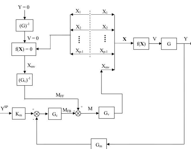
The LNL sandwich model consists of a linear dynamic block followed by a nonlinear static block followed by another linear dynamic block, and is shown in Fig. 2 below.

Figure 2: A block diagram of the LNL sandwich block-oriented model structure. The input vector x passes through the linear dynamic block gi,1 to give the vector v, which then passes

through the nonlinear static map to give w, and finally through the linear dynamic block g2 to

give the output variable y.

Chapter 4 will discuss in more detail the LNL sandwich block-oriented model, and it will be used to identify the process response of a simulated CSTR process with complex input behavior. It will also be used for developing a feedforward controller to be used to maintain control of the reactor temperature of the simulated CSTR process.

4. Statistical Design of Experiments

Although many different approaches have been proposed for addressing both

Hammerstein and Wiener systems, the H-BEST and W-BEST BOM methods first exploited the use of statistical design of experiments (SDOE). The ability to use SDOE ensures that a pure cause-and-effect relationship between inputs and outputs can be obtained [23]. Most methods for identifying Hammerstein and Wiener systems make use of a pseudo-random sequence (PRS), in which a series of deterministic or random input changes occurs at fixed or randomly determined times [36]. If these changes are deterministic, then only a specified number of levels over the input space are used. For the special case of only the minimum and maximum input levels being used in the input sequence, the design is called a pseudo-random binary sequence (PRBS).

gi,1(xi;t,τ) f(v) g2(w;t,τ')

16

Rollins and Bhandari (2004) [21] and Bhandari and Rollins (2003) [19] have

demonstrated that for a simulated process, using SDOE in the model building process gives substantially more information than a PRS design requiring the same amount of experimental test time in the identification process. To demonstrate quantitatively that SDOE is a more efficient method of obtaining significant information, Rollins et al. (2006) [23] introduced an efficiency term to compare the D-optimum criterion (see [37]) for each experimental design type, as applied to Hammerstein processes. In this way, they were able to objectively evaluate competing designs and determine which is more effective. A similar study was done by Hardjasamudra et al. (2006) for Wiener systems [22]. In both of these cases, the authors found that the dynamic parameters could be sufficiently estimated by using a PRS design, but these designs did not allow for the ultimate response behavior to be accurately predicted. Because of this, for BOM development, SDOE appears to be the better choice.

However, in many real processes, making any changes to the inputs for the purpose of developing a reliable process model can cause problems with normal operations. It is

desirable to be able to easily identify the process model without causing significant upsets to the everyday operations of the process. Ideally, historical data from the plant database could be used to develop these models. There are many advantages to using this historical data: the data is readily available and generally abundant, it is collected frequently, it covers the “typical” operating space of the process, and does not require specific perturbations to be introduced, which may cause process upsets. The work done by Rollins et al. [31] which introduced a method of dealing with serially correlated noise has been extended by Rollins et al. [39] to modeling glucose response in Type 2 diabetic patients with highly correlated inputs. Chapter 5 of this dissertation will extend this work further and apply it to modeling

17

the process output response on a real distillation column with highly correlated inputs, and show that an accurate process model can be found using the W-BEST modeling methodology under these conditions. In addition, it will be implemented into a feedforward controller to maintain control of the process output (top tray temperature) on the distillation column,.

5. References

[1] Clarke, D.W., C. Mohtadi and P.S. Tuffs, “Generalized Predictive Control- Part 1: The Basic Algorithm,” Automatica, Vol. 23, pp. 137-148, 1987.

[2] Muske, K.R. and J.B. Rawlins, “Model Predictive Control with Linear Models,”

AIChE Journal, Vol. 39, pp. 262-287, 1993.

[3] te Braake, H.A.B., E.J.L. van Can, J.M.A. Scherpen and H.B. Verbruggen, “Control of Nonlinear Chemical Processes Using Neural Models and Feedback Linearization,”

Computers and Chemical Engineering, Vol. 22, pp. 1113-1127, 1998.

[4] Wright, G.T. and T.F. Edgar, “Nonlinear Model Predictive Control of a Fixed-Bed Water-Gas Shift Reactor: An Experimental Study,” Computers and Chemical

Engineering, Vol 18, pp. 83-102, 1994.

[5] Bodizs, A., F. Szeifert and T. Chovan, “Convolution Model Based Predictive

Controller for a Nonlinear Process,” Industrial and Engineering Chemistry Research, Vol. 38, pp. 154-161, 1999.

[6] Noriega, J.R. and H. Wang, “A Direct Adaptive Neural-Network Control for Unknown Nonlinear Systems and Its Application,” IEEE Transactions on Neural

Networks, Vol. 1, pp. 4-27, 1998.

[7] Alexandridis, A. and H. Sarimveis, “Nonlinear Adaptive Model Predictive Control Based on Self-Correcting Neural Network Models,” AIChE Journal, Vol. 51. No. 9, September 2005.

[8] Fischer, M., O. Nelles and R. Isermann, “Adaptive Predictive Control of a Heat Exchanger Based on a Fuzzy Model,” Control Engineering Practice, Vol. 6, pp. 259-269, 1998.

[9] Di Palma, F., L. Magni, “A Multi-Model Structure for Model Predictive Control,”

18

[10] Gao, J, R. Patwardhan, K. Akamatsu, Y. Hashimoto, G. Emoto, S.L. Shah, B. Huang, “Performance Evaluation of Two Industrial MPC Controllers,” Control Engineering

Practice, Vol. 11, pp.1371-1387, 2003.

[11] Havlena, V. and J. Findejs, “Application of Model Predictive Control to Advanced Combustion Control,” Control Engineering Practice, Vol. 13, pp. 671-680, 2005. [12] Al-Duwaish H. and Naeem, Wasif , “Nonlinear Model Predictive Control of

Hammerstein and Wiener Models Using Genetic Algorithms,” Proceedings of the

2001 IEEE International Conference on Control Applications, September 5-7, 2001,

Mexico City, Mexico

[13] Gao, F., F. Wang and M. Li, “Predictive Control for Processes with Input Dynamic Nonlinearity,” Chemical Engineering Science, Vol. 55, pp. 4045-4052, 2000. [14] Loveland, S.D., Advances in Nonlinear Process Modeling Using Block-oriented

Exact Solution Techniques, M.S. Thesis, Iowa State University, Ames, Iowa 2002.

[15] Pearson, R.K. and B.A. Ogunnaike, “Nonlinear Process Identification,” Nonlinear

Process Control, Prentice-Hall PTR, Upper Saddle River, NJ, pp. 11-110, 1997.

[16] Rollins, D.K., N. Bhandari, A.M. Bassily, G.M. Colver and S. Chin, “A Continuous-Time Nonlinear Dynamic Predictive Modeling Method for Hammerstein Processes,”

Industrial and Engineering Chemistry Research, Vol. 42, No. 4, pp. 861-872, 2003.

[17] Greblicki, W., “Continuous-Time Hammerstein System Identification,” IEEE

Transactions on Automatic Control, Vol. 45, No. 6, pp. 1232-1236, 2000.

[18] Bhandari, N. and D.K. Rollins, “Continuous-Time Hammerstein Nonlinear Modeling Applied to Distillation,” AIChE Journal, Vol. 50, No. 2, pp. 530-533, 2004.

[19] Bhandari, N. and D.K. Rollins, “A Continuous-Time MIMO Wiener Modeling Method,” Industrial and Engineering Chemistry Research, Vol. 42, No. 22, pp. 5583-5595, 2003.

[20] Chin, S., N. Bhandari and D.K. Rollins, “An Unrestricted Algorithm for Accurate Prediction of MIMO Wiener Processes,” Industrial and Engineering Chemistry

Research, Vol. 43, pp. 7065-7074, 2004.

[21] Rollins, D.K. and N. Bhandari, “Constrained MIMO dynamic Discrete-Time Modeling Exploiting Optimal Experimental Design,” Journal of Process Control, Vol. 14, No. 6, pp. 671-683, 2004.

19

[22] Hardjasamudra, A., D.K. Rollins, N. Bhandari and S. Chin, “Optimal Experimental Design for Wiener Systems,” accepted by Chemical Engineering Communications, April, 2006.

[23] Rollins, D.K., L. Pacheco and N. Bhandari, “A Quantitaive Measure to Evaluate Competing Designs for Non-linear Dynamic Process Identification,” The Canadian

Journal of Chemical Engineering, Vol. 84, No. 4, 2006

[24] Zhai, D., Continuous-Time Block-Oriented Nonlinear Modeling with Complex Input

Noise Structure, Ph.D. Dissertation, Iowa State University, Ames, Iowa, 2005.

[25] Narendra, K.S. and P.G. Gallman, “An Iterative Method for the Identification of Nonlinear Systems Using a Hammerstein Model,” IEEE Transactions on Automatic

Control, Vol. 6 (AC-11), pp. 546-550, 1966.

[26] Rollins, D.K., J.M. Liang and P. Smith, “Accurate Simplistic Predictive Modeling of Non-linear Dynamic Processes,” ISA Transactions, Vol. 36, pp. 293-303, 1998. [27] Rietz, C.A., The Application of a Semi-Empirical Modeling Technique to Real

Processes, M.S. Thesis, Iowa State University, Ames, Iowa 1998.

[28] Seborg, D.E., T.F. Edgar and D.A. Mellichamp, Process Dynamics and Control, 2nd edition, John Wiley and Sons, 2003.

[29] Zhai, D., D.K. Rollins and N. Bhandari, “Compact Block-Oriented Continuous-Time Dynamic Modeling for Nonlinear Systems Under Sinusoidal Input Sequences,”

Proceedings of the IASTED Intelligent Systems and Control Conference, Honolulu,

Hawaii, pp. 295-300, 2004.

[30] Zhai, D., D.K. Rollins, N. Bhandari and H. Wu, “Continuous-Time Hammerstein and Wiener Modeling Under Second-Order Static Nonlinearity for Periodic Process Signals,” Computers and Chemical Engineering, Vol. 31, pp.1-12, 2006.

[31] Rollins, D.K., N. Bhandari, S. Chin, T. Junge and K. Roosa, “Optimal Deterministic Transfer Function Modeling in the Presence of Serially Correlated Noise,” Chemical

Engineering Research and Design, Vol. 84(A1), pp. 9-21, 2006.

[32] Huang, H.P., M.W. Lee and Y.T. Tang, “Identification of Wiener Model Using Relay Feedback Test,” Journal of Chemical Engineering of Japan, Vol. 31, No. 4, pp. 604-612, 1998.

20

[33] Balestrino, A. and A. Caiti, “Approximation of Hammerstein/Wiener Dynamic Models,” Proceedings of the IEEE-INNS-ENNS International Joint Conference on

Neural Networks, Vol. 6, Como, Italy, pp. 70-74, 2000.

[34] Brockwell, P.J. and R.A. Davis, Introduction to Time Series and Forecasting, New York: Springer, 2002.

[35] Hajjair, A., and O. Eloutassi, “Extracting Sine Waves from Noisy Measurements and Estimating Their Parameters,” Proceeding of the IASTED Conference on Decision

and Control, pp. 341-345, 1999.

[36] Brosilow, C. and B. Joseph, Techniques of Model-Based Control, Prentice Hall PTR, Upper Saddle River, NJ, pp. 387-394.

[37] Bates, D.M. and D.G. Watts, Nonlinear Regression Analysis and Its Applications, John Wiley & Sons, Inc., New York, NY, pp. 121-133, 1988.

[38] Billings, S.A., “Identification of Nonlinear Systems – A Survey,” IEE Proceedings, Vol. 127 pt.D, No. 6, pp. 272-285, 1980.

[39] Rollins, D.K., J. Kleinedler, A. Strohbehn, L. Boland, M. Murphy, D. Andre, D. Wolf and W.E. Franke, “Modeling Glucose Noninvasively Using Wiener Simulation Modeling for Type 2 Diabetic Patients Under Free-living Conditions,” submitted to

21

CHAPTER 3. PRELIMINARY INVESTIGATIONS

1. Motivation for Research

The process of model identification for model-based control algorithms takes on many different forms, depending upon the type of model to be used. In this research, the focus will be on block-oriented models, which combine linear dynamic (L) and nonlinear static (N) blocks to approximate nonlinear process response behavior. Most of the methods for identifying block-oriented models make use of a pseudo-random sequence (PRS). The PRS consists of a series of deterministic or random input changes occurring at fixed or randomly determined times [1]. Studies have been done by Rollins et al. [2] and Hardjasaumdra et al. [3] that showed that while dynamic parameters can be sufficiently estimated by using a PRS design, the ultimate response behavior of a process is not

accurately predicted using the PRS design. This contributes to process-model mismatch that will negatively affect performance of a model-based controller.

In a real process, the inputs are usually not stepwise deterministic. They often have periodic and stochastic behavior. This has been noted and some work has been done to properly identify models for systems that have periodic inputs [4, 5] or serially correlated inputs [6, 7]. However, the general equations for model-based control do not explicitly account for these types of inputs. In addition, the inputs to a process typically have a dynamic response to controller set point changes and not an instantaneous, constant-level response. Dynamic interactions between the input variables exist in many processes, and these are also not explicitly accounted for. Instead, any dynamic or interactive behavior of the inputs contributes to mismatch of the overall process model.

22

To illustrate the effect of input dynamics, consider a simple two-input, one-output Hammerstein process. We could express this in block diagram form as in Fig. 1.

Figure 1: The block diagram for a simple two-input, one-output Hammerstein process. The inputs are represented by X1sp and X2sp, v is the intermediate vector representing the static

map of X and Y is the output.

In this example, the set points are given by X1sp and X2sp. If there are input dynamics,

then the block diagram would need to be modified, as in Fig. 2. This accounts for both input dynamics and the process dynamics. Essentially this is what is known as a sandwich block-oriented model (BOM), in which linear dynamic blocks and static nonlinearities can be assembled in any of a number of arrangements [8]. The process represented by Fig. 2 is considered an LNL sandwich process, in which the input goes through a linear dynamic block, then a nonlinear static block and finally another linear dynamic block. If the input dynamics can be separated from the process dynamics in the modeling of the process that is done for the control system, the overall control and stability of the process could be better maintained.

f(X) v G(s) Y(s)

X1sp (s) X2sp (s)

23 Y(s) f(X) v G(s) X1(s) X2(s) G1(s) G2(s) X1sp (s) X2sp (s) Y(s)

Figure 2: The block diagram for a two-input, one-output LNL sandwich process that has input dynamic behavior. The input set points have been modified to show the dynamic response of the inputs to the set point changes.

2. Scope of Research

As discussed previously, the inputs to a process are often nonstationary. If we consider this variability to be significant, we can break the input signal up into three specific parts: dynamic, periodic and stochastic contributions to noise. Mathematically, the

variability can be represented by Eq. 1 below. It can also be described in block-diagram form, with the input xi(t) entering into a Hammerstein system in Fig. 3.

( )

( )

( )

( )

x_i = _i +ε_i +ξ_i (1)

where xi(t) represents the input, wi(t) represents the dynamic contribution, εi(t) represents the

stochastic contribution and ξi(t) represents the periodic contribution to the process variability.

Figure 3: A block diagram representing an LNL sandwich system with input process variability consisting of three parts: dynamic, stochastic and periodic.

Y( f(xi) gi(t) vi xi(t) gisp(s) xisp (t) yi(t) εi wi ₊ + + ξi

24

All three contributions to the input process variability are often due to real process variability. However, the research presented in this dissertation will focus on one of the two deterministic components, the dynamic component. The goal is to model these contributions and implement them into a model-based control scheme. Zhai [5] has proposed methods for handling the stochastic component.

The examples to be investigated include a simulated true LNL sandwich process, a simulated continuous-stirred tank reactor (CSTR) process and a real distillation process. The true LNL sandwich process will be used to illustrate the importance of understanding the input dynamics and the effects of interactive inputs. Using the simulated CSTR process, an LNL block-oriented model will be developed and implemented into a feedforward/feedback control algorithm. This will be compared to the performance of a traditional feedback controller, and is shown in Chapter 4. For the pilot-scale distillation column we will identify a Wiener block-oriented model in both open- and closed-loop modes using data typical of what could be found in a plant historical database, and implement this model into a feedforward/feedback control scheme to show the response of the process output.

Comparisons will be made between this and a traditional feedback control system. This is given in Chapter 5.

3. Preliminary Work

3.1. Example 1: Simulated NL Process

To demonstrate that the dynamics of the process inputs can have a significant effect on the process response, let us consider a simple two-input, single-output NL (Hammerstein) process. This process is defined by Eqs. 2 and 3 and is illustrated by the block diagram shown in Fig. 1 above.

25

( )

( )

( )

( )

_{( )}

_{( )}

In this case, all initial conditions and derivatives are equal to zero, a0= 2.0, a1= 0.5, a2=

0.75, a3= 1.0, a4= 2.5, a5= -0.5, τw = 5.0 and θw = 2.0. An arbitrary set of input set point

changes were made to the process using a random number generator with a uniform

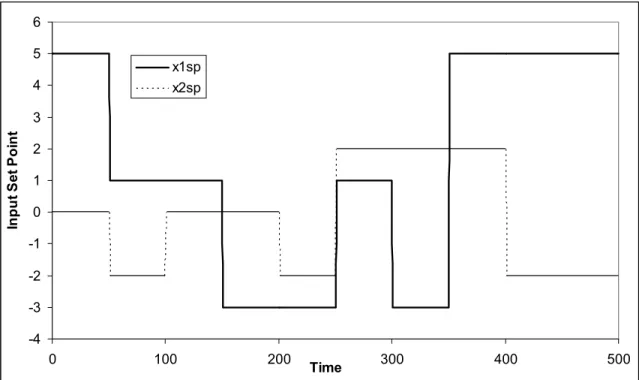
distribution. This input sequence is shown in Fig. 4. If these set point changes are the true input changes to the process, then the output response to the changes is given in Fig. 5.

-4 -3 -2 -1 0 1 2 3 4 5 6 0 100 200 300 400 500 Time In p u t Se t Po in t x1sp x2sp

Figure 4: The set point changes made to the inputs x1 and x2 used in the simulated NL

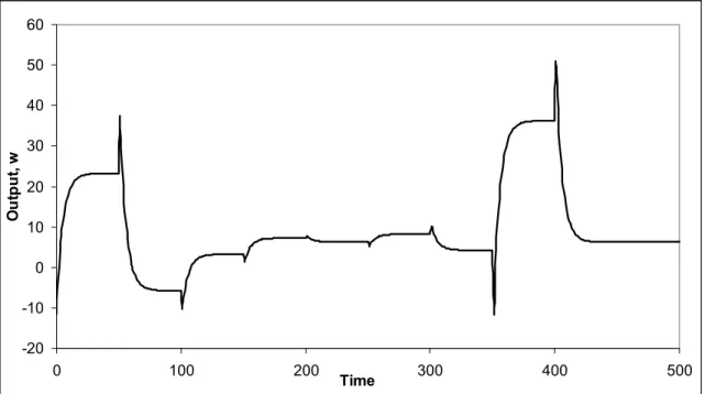
26 -20 -10 0 10 20 30 40 50 60 0 100 200 300 400 500 Time Ou tp u t, w

Figure 5: The simulated NL process output response to the input changes that are shown in Figure 4.

3.2. Example 2: Simulated LNL Process

In many cases, however, there is dynamic behavior in the measured input to a process as compared to the changes in the input set points that occur. The process is then an LNL process, depicted in Fig. 2 above. Suppose that each of the two inputs in our NL process exhibit simple second-order overdamped dynamic behavior, as represented in Eqs. 4 and 5 below:

( )

₍

₎₍

₎

( )

₍

₎₍

₎

where xi and xisp represent the ith input and ith input set point values, respectively. In the

27

Graphically, the dynamic change in the inputs is shown in Fig. 6. We can see that the input to the process is now much different than what was given by the set point changes alone. Because of this, the output response of the process is also significantly different, and is shown in Fig. 7. -4 -3 -2 -1 0 1 2 3 4 5 6 0 100 200 300 400 500 Time Input S e t P oi nt x1sp x2sp x1 x2

Figure 6: The inputs x1 and x2 are shown along with their set point changes. Each of the

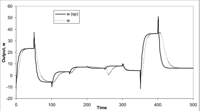
28 -20 -10 0 10 20 30 40 50 60 0 100 200 300 400 500 Time O ut put , w w (sp) w

Figure 7: The simulated process output response, w, shown for both the pure set point changes (the NL process) and for inputs that have a dynamic response to the set point changes (the LNL process).

3.3. Example 3: Interactive Effects of Inputs

In addition to the dynamic behavior of inputs that can exist, there can also be

interactive effects of the inputs on the process. The steady-state interactions are addressed in BOM by the nonlinear static block, which can be any nonlinear function. In the simulated LNL process that we have been discussing, this can be easily seen by holding one of the inputs constant while changing the other one. That is, if we use the same input sequence for x1 that we have already introduced in Fig. 4 but keeping x2 constant, we can see the process

response to the changes in x1. The ultimate response of the process to these changes is

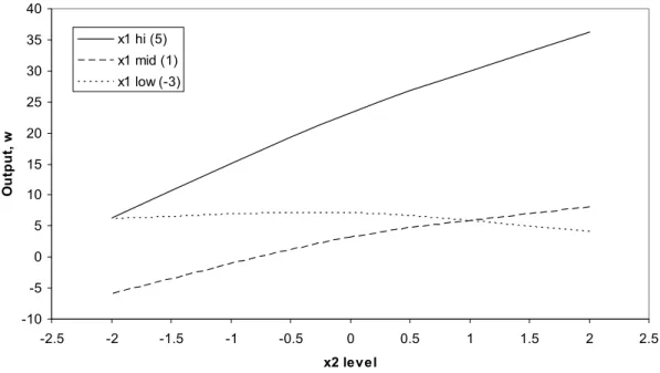
shown in Fig.8. Note that since the lines are not parallel, there is an interaction between the two inputs. The same is true if we hold x1 constant while changing x2.

29 -10 -5 0 5 10 15 20 25 30 35 40 -2.5 -2 -1.5 -1 -0.5 0 0.5 1 1.5 2 2.5 x2 level Ou tp u t, w x1 hi (5) x1 mid (1) x1 low (-3)

Figure 8: The ultimate response of the output, w, given by the simulated LNL process to changes in the two inputs, x1 and x2. The intersection of the lines demonstrates an interaction

between the two inputs.

This interaction also has an effect on the dynamics of the process. We can see in Fig. 9 that the dynamics vary depending on whether x1, x2 or both are changing.

Again, by understanding the dynamics of the interactions between the two inputs and modeling these explicitly using an LNL BOM, we should be able to maintain better control of the process than if we use a Hammerstein or Wiener model within a model predictive control scheme.

30 -10 -5 0 5 10 15 20 25 30 35 40 0 100 200 300 400 500 Time Ou tp u t, w w (x1 only) w (x2 only) w (both)

Figure 9: The simulated LNL process output response to input changes in x1 only, x2 only,

and both x1 and x2. This shows the interactive effect that changing both input variables has

on the output, w.

3.4. Example 4: A Pilot-Scale Distillation Process

Tests were conducted on a pilot-scale distillation column to demonstrate the dynamic behavior of the inputs on a real process. The column is used to separate a mixture of

methanol and water, and is shown schematically in Fig. 10. The column consisted of 12 sieve trays and had an inside diameter of 6 inches.

31

Figure 10: The distillation column used for the experimental tests. The column separated methanol and water and was operated by a DeltaV distributed control system [9].

32

The input variables to the process include the feed flow rate, feed temperature,

reboiler steam pressure, reboiler level and reflux flow rate. Other inputs that were considered were the distillate flow rate, bottoms flow rate and overhead temperature; however, these were not included in the experimental design. The distillate flow and overhead temperature were held constant, and the bottoms flow rate was cascaded with the reboiler level in order to maintain proper control of the column. In addition, although there are three possible feed trays, for these experiments the feed was only introduced on tray 6 in the middle of the column. The output variable examined was the top tray (Tray 12) temperature, from which a composition could be inferred.

A statistical experimental design was determined and carried out on the distillation column. The design was a Box-Behnken design [10] with four factors and three center points, resulting in a total of 27 runs. The four inputs that were manipulated were the feed flow rate, the feed temperature, the reboiler level and the reboiler steam pressure. It is important to note that we also consider reflux flow rate to be an input to the process. It was not specifically manipulated for the experiments because doing so may have caused

instability in the operation of the column. Instead, the reflux flow rate is cascaded to an overhead condensate accumulator level controller. In the modeling of the distillation column that will be performed, we will consider this flow as an input, but it could not be included as part of the design due to safety and operational reasons.

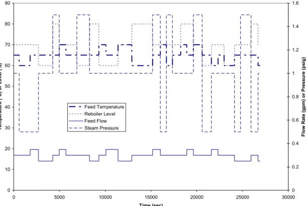
The experimental design is shown in Fig. 11. Note that Fig.11 shows the set point changes for each of the inputs. The measured value of each of the inputs that was varied in the experiment showed significant dynamic behavior.

33 0 10 20 30 40 50 60 70 80 90 0 5000 10000 15000 20000 25000 30000 Time (sec) T em p erat u re ( °C) o r L evel ( % ) 0 0.2 0.4 0.6 0.8 1 1.2 1.4 1.6 F lo w R at e ( g p m ) o r P ressu re ( p si g ) Feed Temperature Reboiler Level Feed Flow Steam Pressure

Figure 11: The set point changes used for the experimental design of the distillation column. The design used was a Box-Behnken design with 27 points.

The measured responses of the inputs to their set point changes can be seen in Figures 12 through 15, and the dynamic behavior of these inputs is clearly visible in these plots.

34 0 0.2 0.4 0.6 0.8 1 1.2 1.4 1.6 1.8 2 0 5000 10000 15000 20000 25000 Time P ress u re ( p si g ) PV SP

Figure 12: Reboiler steam pressure response to the set point changes made during the experiments that were conducted on the distillation column. SP represents the change in set point and PV represents the measured process value of the reboiler steam pressure.

50 55 60 65 70 75 80 85 90 0 5000 10000 15000 20000 25000 Time (sec) R eboile r Le ve l (% ) SP PV

Figure 13: Reboiler level response to the set point changes made during the experiments that were conducted on the distillation column. SP represents the change in set point and PV represents the measured process value of the reboiler level.

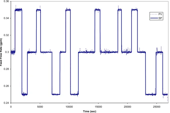
35 0.24 0.26 0.28 0.3 0.32 0.34 0.36 0 5000 10000 15000 20000 25000 Time (sec) Fe ed F low Ra te (gp m ) PV SP

Figure 14: Feed flow response to the set point changes made during the experiments that were conducted on the distillation column. SP represents the change in set point and PV represents the measured process value of the feed flow rate.

58 60 62 64 66 68 70 72 74 76 78 0 5000 10000 15000 20000 25000 Time (sec) Fe ed Te m p ( °C ) SP PV

Figure 15: Feed temperature response to set point changes during the experiments that were conducted on the distillation column. SP represents the change in set point and PV

36

Based upon our previous discussion of the variability in a process input, we can see from these figures that each of the inputs on the distillation column behave according to different combinations of the three variability contributions. The reboiler level and feed temperature inputs appear to demonstrate significant dynamic behavior, while the feed flow and steam pressure inputs do not.

Let us examine more closely the feed temperature input. This one is of particular interest because the feed temperature is affected not only by the set point changes of the feed temperature controller, but also by changes in the feed flow rate. Fig. 15 shows the input sequence for the set point changes in feed temperature along with the feed temperature that was measured during the experiments.

The H-BEST model algorithm introduced by Rollins, et al. (1998) [11] was used to fit the temperature data. For one change occurring at t = 0, this can be written as

( )

t

f

(

u

( )

t

) ( ) ( )

g

t

t

y

=

;

β

⋅

;

τ

s

where β is the vector of coefficients and the dynamics are described by g(t;τ). It is important to note that in this case the function f(u(t);β) is equal to 1 because the input is a set point and the output is the process response to set point. Therefore, we essentially have only the dynamic block to model the process response. The dynamic behavior of the process was fit to a second-order underdamped model, which is represented as

( )

(

)

(

)

_ζ

_τ

ζ

ζ

τ

ζ

37

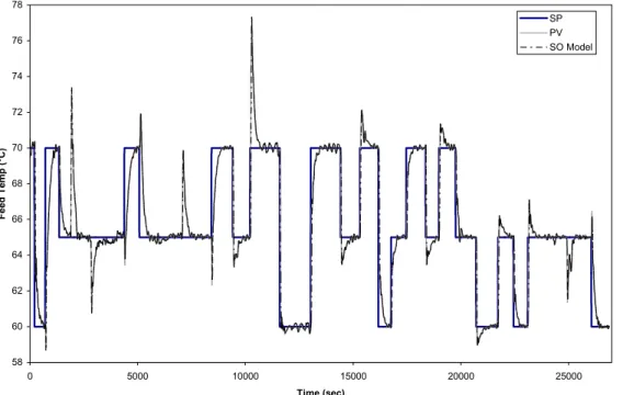
The parameters found for this model of the process were τˆ = 1.49 and ζˆ = 0.659. The fit of the model to the process can be seen in Fig. 16. As this demonstrates, the model did a very good job of fitting the process data.

58 60 62 64 66 68 70 72 74 76 78 0 5000 10000 15000 20000 25000 Time (sec) Fe ed T em p ( °C ) SP PV SO Model

Figure 16: The feed temperature response (PV) to the set point changes (SP) introduced during the experimental runs, along with the second-order underdamped model (SO Model) fit to the feed temperature.

4. Dissertation Research

The questions to be addressed in this research are the following: how do we include this input information into a model-based control algorithm without requiring excessive computational effort? How will this work on a process that has multiple inputs? Can we develop a practical method for identifying the model and implementing it into a model-based control algorithm without requiring any extra model identification effort? These questions will be addressed in detail in the forthcoming chapters.

38

The goal was to ultimately implement the models developed into a model-based control scheme on the pilot-scale distillation column that was discussed earlier, and use that control algorithm to maintain product quality. The pilot-scale distillation column initially had no overall composition control but instead used several individual controllers to maintain specific operating parameters. Steps will be taken toward achieving the ultimate goal by first testing a new feedforward/feedback control algorithm on a simulated continuous-stirred tank reactor (CSTR) process that can be adequately modeled by an LNL block-oriented model. This is demonstrated in Chapter 4. The control scheme will then be developed further, to show that the models can be identified using data similar in nature to plant historical data, and then implemented into a feedforward/feedback control algorithm that will be applied to the pilot-scale distillation process in the laboratory. Chapter 5 discusses the methods for identifying the model and applying the control scheme to the distillation process.

5. References

[1] Brosilow, C. and B. Joseph, Techniques of Model-Based Control, Prentice Hall PTR, Upper Saddle River, NJ, pp. 387-394.

[2] Rollins, D.K., L. Pacheco and N. Bhandari, “A Quantitaive Measure to Evaluate Competing Designs for Non-linear Dynamic Process Identification,” The Canadian

Journal of Chemical Engineering, Vol. 84, No. 4, 2006

[3] Hardjasamudra, A., D.K. Rollins, N. Bhandari and S. Chin, “Optimal Experimental Design for Wiener Systems,” accepted by Chemical Engineering Communications, April, 2006.

[4] Zhai, D., D.K. Rollins and N. Bhandari, “Compact Block-Oriented Continuous-Time Dynamic Modeling for Nonlinear Systems Under Sinusoidal Input Sequences,”

Proceedings of the IASTED Intelligent Systems and Control Conference, Honolulu,

39

[5] Zhai, D., Wu and D.K. Rollins, “Parameter Estimation for the Wiener Dynamic System With Unmeasured Continuous-Time Correlated Stochastic Disturbances,” submitted to Industrial and Engineering Chemistry Research, September, 2005, in review.

[6] Zhai, D., D.K. Rollins, N. Bhandari and H. Wu, “Continuous-Time Hammerstein and Wiener Modeling Under Second-Order Static Nonlinearity for Periodic Process Signals,” Computers and Chemical Engineering, in press.

[7] Rollins, D.K., N. Bhandari, S. Chin, T. Junge and K. Roosa, “Optimal Deterministic Transfer Function Modeling in the Presence of Serially Correlated Noise,” Chemical

Engineering Research and Design, Vol. 84(A1), pp. 9-21, 2006.

[8] Pearson, R.K. and B.A. Ogunnaike, “Nonlinear Process Identification,” Nonlinear

Process Control, Prentice-Hall PTR, Upper Saddle River, NJ, pp. 11-110, 1997.

[9] Loveland, S.D. and L. dela Rosa, “Distillation – A Unit Operations Laboratory Manual,” Department of Chemical and Biological Engineering, Iowa State University, Ames, Iowa, 2005.

[10] Cochran, W.G. and G. Cox, Experimental Designs, 2nd ed., Wiley, New York, 1992. [11] Rollins, D.K., J.M. Liang and P. Smith, “Accurate Simplistic Predictive Modeling of

40

CHAPTER 4. NONLINEAR MULTIPLE INPUT FEEDFORWARD

CONTROL UNDER BLOCK-ORIENTED MODELING

A paper to be submitted to the Journal of Process Control

Stephanie D. Loveland, Derrick K. Rollins and Nidhi Bhandari

1. Background

The control of chemical processes is a very important part of an industrial plant. Traditional feedback control makes adjustments to some manipulated variable after the process has deviated from its desired operating condition. In the past few decades, more sophisticated control algorithms have been introduced that use predictive models to correct for disturbances before a deviation of the process output from its set point occurs. Many of these are model-based control algorithms, including feedforward control, internal model control and model predictive control (MPC). Each of these types of model-based control uses a model of the process. In most instances, these control algorithms use linear models to predict process behavior based on input changes. However, many real processes exhibit complicated nonlinear behavior so these linear estimations are limited as to when they can be used. Therefore, the use of linear models is often restricted to certain input or output ranges [1, 2].

Some nonlinear models have been proposed for model-based controllers, including artificial neural networks (ANNs) and radial basis functions (RBF) [3, 4], genetic algorithms (GA) [5] and NARMAX models [6, 7, 8]. Another type of nonlinear model that has been used is a block-oriented model (BOM) [9-14], which combines blocks of static nonlinearities with blocks of linear dynamics. The simplest of the block-oriented models are the