Donald L. Simon
Glenn Research Center, Cleveland, Ohio
Jeffrey B. Armstrong
ASRC Aerospace Corporation, Cleveland, Ohio
Sanjay Garg
Glenn Research Center, Cleveland, Ohio
Application of an Optimal Tuner Selection
Approach for On-Board Self-Tuning Engine Models
NASA/TM—2012-217278
GT2011–46408
NASA STI Program . . . in Profile
Since its founding, NASA has been dedicated to the advancement of aeronautics and space science. The NASA Scientific and Technical Information (STI) program plays a key part in helping NASA maintain this important role.
The NASA STI Program operates under the auspices of the Agency Chief Information Officer. It collects, organizes, provides for archiving, and disseminates NASA’s STI. The NASA STI program provides access to the NASA Aeronautics and Space Database and its public interface, the NASA Technical Reports Server, thus providing one of the largest collections of aeronautical and space science STI in the world. Results are published in both non-NASA channels and by NASA in the NASA STI Report Series, which includes the following report types:
• TECHNICAL PUBLICATION. Reports of completed research or a major significant phase of research that present the results of NASA programs and include extensive data or theoretical analysis. Includes compilations of significant scientific and technical data and information deemed to be of continuing reference value. NASA counterpart of peer-reviewed formal professional papers but has less stringent limitations on manuscript length and extent of graphic presentations.
• TECHNICAL MEMORANDUM. Scientific and technical findings that are preliminary or of specialized interest, e.g., quick release reports, working papers, and bibliographies that contain minimal annotation. Does not contain extensive analysis.
• CONTRACTOR REPORT. Scientific and technical findings by NASA-sponsored contractors and grantees.
• CONFERENCE PUBLICATION. Collected papers from scientific and technical
conferences, symposia, seminars, or other meetings sponsored or cosponsored by NASA. • SPECIAL PUBLICATION. Scientific,
technical, or historical information from NASA programs, projects, and missions, often concerned with subjects having substantial public interest.
• TECHNICAL TRANSLATION. English-language translations of foreign scientific and technical material pertinent to NASA’s mission. Specialized services also include creating custom thesauri, building customized databases, organizing and publishing research results.
For more information about the NASA STI program, see the following:
• Access the NASA STI program home page at
http://www.sti.nasa.gov
• E-mail your question via the Internet to help@
sti.nasa.gov
• Fax your question to the NASA STI Help Desk at 443–757–5803
• Telephone the NASA STI Help Desk at 443–757–5802
• Write to:
NASA Center for AeroSpace Information (CASI) 7115 Standard Drive
Donald L. Simon
Glenn Research Center, Cleveland, Ohio
Jeffrey B. Armstrong
ASRC Aerospace Corporation, Cleveland, Ohio
Sanjay Garg
Glenn Research Center, Cleveland, Ohio
Application of an Optimal Tuner Selection
Approach for On-Board Self-Tuning Engine Models
NASA/TM—2012-217278
GT2011–46408
National Aeronautics and
Space Administration
Glenn Research Center
Cleveland, Ohio 44135
Prepared for the
Turbo Expo 2011
sponsored by the American Society of Mechanical Engineers (ASME)
Vancouver, British Columbia, Canada, June 6–10, 2011
Acknowledgments
This research was conducted under the NASA Aviation Safety Program, Vehicle Systems Safety Technologies Project. The authors gratefully acknowledge Jonathan Litt for his support and insightful discussions which led to the development of this work.
Available from NASA Center for Aerospace Information
7115 Standard Drive Hanover, MD 21076–1320
National Technical Information Service 5301 Shawnee Road Alexandria, VA 22312 Available electronically at http://www.sti.nasa.gov
Application of an Optimal Tuner Selection Approach
for On-Board Self-Tuning Engine Models
Donald L. Simon
National Aeronautics and Space Administration Glenn Research Center
Cleveland, Ohio 44135
Jeffrey B. Armstrong ASRC Aerospace Corporation
Cleveland, Ohio 44135
Sanjay Garg
National Aeronautics and Space Administration Glenn Research Center
Cleveland, Ohio 44135
Abstract
An enhanced design methodology for minimizing the error in on-line Kalman filter-based aircraft engine performance estimation applications is presented in this paper. It specific-ally addresses the underdetermined estimation problem, in which there are more unknown parameters than available sensor measurements. This work builds upon an existing technique for systematically selecting a model tuning para-meter vector of appropriate dimension to enable estimation by a Kalman filter, while minimizing the estimation error in the parameters of interest. While the existing technique was optimized for open-loop engine operation at a fixed design point, in this paper an alternative formulation is presented that enables the technique to be optimized for an engine operating under closed-loop control throughout the flight envelope. The theoretical Kalman filter mean squared estimation error at a steady-state closed-loop operating point is derived, and the tuner selection approach applied to minimize this error is discussed. A technique for constructing a globally optimal tuning parameter vector, which enables full-envelope applica-tion of the technology, is also presented, along with design steps for adjusting the dynamic response of the Kalman filter state estimates. Results from the application of the technique to linear and nonlinear aircraft engine simulations are presented and compared to the conventional approach of tuner selection. The new methodology is shown to yield a signifi-cant improvement in on-line Kalman filter estimation accuracy.
Introduction
An emerging approach in the field of aircraft engine ctrols and health management is the inclusion of real-time on-board adaptive models for the in-flight estimation of engine performance parameters (Refs. 1 to 3). These models, typically based on Kalman filters, enable the estimation of
unmeasured engine performance parameters that can be used for diagnostics, prognostics, and controls applications. A challenge that complicates this practice is the fact that an aircraft engine’s performance is affected by its level of degradation, generally described in terms of unmeasurable health parameters such as efficiencies and flow capacities related to each major engine module. The level of engine performance degradation can be estimated using a Kalman filter, given that there are at least as many sensors as parame-ters to be estimated (Ref. 4). However, in an aircraft engine the number of sensors available is typically less than the number of health parameters, presenting an under-determined estimation problem. The conventional approach to address this shortcoming is to estimate a subset of the health parameters, referred to as model tuning parameters. While this approach enables on-line Kalman filter-based estimation, it can introduce error in the accuracy of overall model-based performance estimation applications. In a departure from the conventional approach of selecting a subset of health parame-ters to serve as the tuner vector, Litt (Ref. 5) presented a novel approach based on singular value decomposition that selects a model tuning parameter vector of low-enough dimension to be estimated by a Kalman filter. In this method, a model tuning parameter vector, q, is constructed as a linear combination of all health parameters, h, given by
q = V*h (1)
where the transformation matrix, V*, is selected by applying singular value decomposition to capture the overall effect of the larger set of health parameters on the engine variables as closely as possible in the least squares sense. An enhancement to the work of Litt, presented by Simon and Garg (Ref. 6), selects V* to minimize the theoretical mean squared estimation error in the parameters of interest at a steady-state open-loop linear design point.
In this paper, several design enhancements to the optimal tuner selection methodology presented in Reference 6 are
discussed and presented. These include extending the optimal tuner selection methodology to encompass closed-loop control operating conditions, selection of a single tuner vector for application throughout the engine operating envelope as opposed to at a single design point, and design considerations to provide the desired Kalman filter dynamic response. The remainder of this paper is organized as follows. First, some mathematical preliminaries are given regarding the problem formulation including the linear model representing system dynamics and the formulation of the Kalman filter. Next, several practical design considerations are discussed including an approach for selecting a tuner vector optimal for full-envelope operation, referred to as a globally optimal tuner vector, and design steps for adjusting Kalman filter dynamic response. This is followed by an example application of the methodology to linear and nonlinear turbofan engine simula-tions. Finally, conclusions are presented.
Nomenclature
A, Ac, Axh, Axq, B, Bce, Bco, Bxh, Bxq, C, Cc, Cxh, Cxq, D, F, Fxh, Fxq, G, L, M, N system matricesC-MAPSS Commercial Modular Aero-Propulsion System Simulation
Fn net thrust
HPC high pressure compressor HPT high pressure turbine
I identity matrix
K∞ Kalman filter gain LPC low pressure compressor LPT low pressure turbine
Ph health parameter covariance matrix
PLA power lever angle
PWLKF piece-wise linear Kalman filter
P∞ Kalman filter state estimation covariance
matrix
Q, Qxh, Qxq process noise covariance matrices
R measurement noise covariance matrix SmLPC low pressure compressor stall margin
SSEE sum of squared estimation errors
V* transformation matrix relating hk to qk
WSSEE weighted sum of squared estimation errors
e error between control setpoint and feedback
signal
h health parameter vector
m number of measured outputs
p number of health parameters
q Kalman filter tuning parameter vector
r control setpoint
u actuator command vector
v measurement noise vector
w, wh, wxh, wxq process noise vectors
x, xxh, xxq state vectors
y vector of measured outputs
z vector of unmeasured (auxiliary) outputs
Subscripts
c control parameter
k discrete time step index
o open-loop feedback signal
r feedback signal
xh augmented state vector (x and h)
xq reduced order state vector (x and q)
ss steady-state value Superscripts † pseudo-inverse T transpose - a priori estimate + a posteriori estimate Diacritical marks ˆ estimated value ˘ augmented ˜ error or residual ˉ expected or mean value
Problem Formulation
The discrete linear time-invariant engine state space equa-tions about a design point are given as
1 k k k k k k k k k k k k k k x Ax Bu Lh w y Cx Du Mh v z Fx Gu Nh + = + + + = + + + = + + (2)
where k is the time index, x is the vector of state variables, u is the vector of control inputs, y is the vector of measured outputs, z is the vector of auxiliary (unmeasured) model outputs, and h is the vector of engine health parameters. The vectors w and v are zero-mean white noise inputs, with covariance of Q and R, respectively. The matrices A, B, C, D,
F, G, L, M, and N are of appropriate dimension. From Eq. (2) it can readily be observed that health parameter deviations induce shifts in the engine state variables and outputs. As such, health parameter effects must be accounted for to achieve accurate engine performance estimation. Towards this requirement, Eq. (2) can be rewritten such that h is concate-nated with x to form an augmented state vector, xxh, as shown
in Eq. (3). Since engine performance deterioration is very slowly evolving relative to other engine dynamics, h is here modeled without dynamics.
[
]
[
]
, , , , 1 , 1 , , , , 0 0 xh xh k xh xh k xh xh k xh xh k k k k k h k k k B x A w xh xh k xh k xh k k k k k k C x xh xh k k k k k k k F x xh xh k k w x A L x B u w h I h A x B u w x y C M Du v h C x Du v x z F N Gu h F x Gu + + = + + = + + = + + = + + = + = + (3)The vector wxh is zero-mean white noise associated with the
augmented state vector, [xThT]T, with a covariance of Qxh. wxh
consists of the original state process noise, w, concatenated with the process noise associated with the health parameter vector, wh. , , k xh k h k w w w = (4)
Closed-Loop State-Space Model
This paper considers an engine operating under closed-loop control conditions. As a point of introduction, refer to the architecture shown in Figure 1 depicting the interaction between an aircraft engine, a controller, and a Kalman filter. Here, the controller accepts inputs consisting of an error signal, ek, (i.e., a residual between a commanded parameter, rk,
and a sensed feedback parameter, yr,k), along with additional sensed measurements, yo,k. The controller processes these
inputs to produce actuator commands, uk.
As shown in Figure 1, engine operation is effected by both actuator commands and the engine’s level of deterioration denoted by the unknown set of health parameter inputs, hk.
Controller AircraftEngine
rk ek uk yk yr,k + -zk hk Kalman Filter ˆ ,ˆ ,ˆ , ˆ ˆ , k k k k k x y z q h yo,k uk
Figure 1.—Aircraft engine, controller, and Kalman filter.
The Kalman filter processes the measurements, yk,
and actuator commands, uk, to produce the estimates
ˆ ˆk, ˆk,ˆk,ˆk, and k
x y z q h .
The controller state space equations are given as
, 1 , , , , c k c c k ce k co o k k c c k k k r k x A x B e B y u C x e r y + = + + = = − (5)
and the sensed feedback parameters, yr,k and yo,k, can be
written as , , r k r k r k r k o k o k o k o k y C x D u M h y C x D u M h = + + = + + (6)
From Eqs. (5) and (6) the controller state variables become
(
)
(
)
(
)
(
)
(
)
, , 1 , , ... ... ... k o k c k c c k ce k r k r k r k e co o k o k o k y c c k ce r co o k ce r co o k ce r co o k ce k x A x B r C x D u M h B C x D u M h A x B C B C x B D B D u B M B M h B r + = + − − − + + + = + − + + − + + − + + (7)Substituting uk = Ccxc,k (from Eq. (5)) into Eq. (7) yields
(
)
(
)
(
)
1 2 1 , 1 , ... ... c k ce r co o k A c ce r c co o c c k A ce r co o k ce k L x B C B C x A B D C B D C x B M B M h B r + = − + + − + + − + + (8)From Eqs. (2) and (5) the closed-loop engine state variables can be written as
(
)
1 , k k k c c k k u x+ =Ax +B C x +Lh (9)The quantities in Eqs. (8) and (9) can be augmented with the health parameters to obtain
1 , 1 1 2 1 , 1 0 0 0 0 k c k c k c k ce k k k x A BC L x x A A L x B r I h h + + + = + (10)
For simplicity the following augmented matrices and vectors are defined , 1 2 1 0 k k c k c ce x x x A BC A A A B B L L L = = = = (11)
allowing the closed-loop state space equations to be re-written in the following form using Eqs. (2), (5), (10), and (11)
1 1 , , 0 0 k k k k k k k k c c k k u k c C k k c c k k u k c F x A L x B r h I h y Cx D C x Mh x C DC M h z Fx G C x Nh x F GC N h + + = + = + + = = + + = (12)
Reduced-Order State Space Model
To enable Kalman filter formulation when presented the underdetermined estimation problem a reduced-order state space model must be constructed. This is accomplished by
defining a model tuning parameter vector, q, which is a linear combination of all health parameters, h, given by
*
q=V h (13)
where q∈ m, h∈ p, m < p, and V* is an m×p transforma-tion matrix of rank m, applied to construct the tuning parame-ter vector. While q is constructed as a linear combination of health parameters, the elements of q do not have any physical meaning. Their purpose is to allow an accurate estimation of unmeasured engine parameters. However, given q, an approximation of the health parameter vector, hˆ, can be obtained as
*† ˆ
h=V q (14)
where V*† is the pseudo-inverse of V*. Substituting Eq. (14) into Eq. (3) yields the following reduced order state space equations which will be used to formulate the Kalman filter
, , , , *† 1 , 1 , , *† , *† 0 0 xq xq k xq xq k xq xq k xq xq k k k k k q k k k B x A w xq xq k xq k xq k k k k k k C x xq xq k k k k k k F x w x A LV x B u w q I q A x B u w x y C MV Du v q C x Du v x z F NV q + + = + + = + + = + + = + + = , k xq xq k k Gu F x Gu + = + (15)
For the reduced order system, the state process noise, wxq, and
its associated covariance, Qxq, are calculated as
, * , * , * * 0 0 0 0 0 0 0 0 k xq k xh k h k T xq xh w I I w w w V V I I Q Q V V = = = (16)
Kalman Filter Formulation
In this study, steady-state Kalman filtering is applied. This means that while the Kalman filter is a dynamic system, the state estimation error covariance matrix and the Kalman gain matrix are time invariant—instead of updating these matrices each time step they are pre-converged and held constant at
their final values. Given the reduced order linear state space equations shown in Eq. (15), the state estimation error covariance matrix, P∞, is calculated by solving the following Riccati equation (Ref. 7)
1 ( ) T T T xq xq xq xq xq xq T xq xq xq P A P A A P C C P C R C P A Q − ∞ ∞ ∞ ∞ ∞ = − + × + (17)
The steady-state Kalman filter gain, K∞, can then be calculated as follows (Ref. 7) 1 ( ) T T xq xq xq K∞ =P C∞ C P C∞ +R − (18)
The Kalman filter a priori and a posteriori estimates are given in Eq. (19) and Eq. (20) respectively (Ref. 7)
, , 1 1 ˆxq k xqˆxq k xq k x− =A x+ − +B u− (19)
(
)
, , , ˆxq k ˆxq k k xqˆxq k k x+ =x− +K∞ y −C x− −Du (20)The reduced order state vector a posteriori estimate, xˆxq k+, , produced by Eq. (20) can be used to produce an estimate of the augmented state vector and the auxiliary parameters as follows , *† , *† , 0 ˆ ˆ 0 ˆ ˆ xh k xq k k xq k k I x x V z F NV x Gu + + = = + (21)
Optimal Transformation Matrix Selection
As presented in Reference 6, the estimation accuracy of the Kalman filter is directly dependent on the selection of the transformation matrix, V*. This gives rise to the optimization problem of selecting V* to minimize the estimation error in the parameters of interest. This can be accomplished by conduct-ing an optimal iterative search to select a V* matrix that minimizes the mean sum of squared estimation errors (SSEE) in the parameters of interest
( )
* * arg min m p V SSEE V × ∈ (22)Alternatively, a weighted mean sum of squared estimation errors, WSSEE, can be applied to place more/less emphasis on certain parameters, or to account for variation in the engineer-ing units of different parameters. Reference 6 presented derivations of health parameter and auxiliary parameter mean
SSEE as a function of V* at an open-loop steady-state operat-ing point. While the functional design of a Kalman filter applied to an open-loop versus a closed-loop system is the same due to the separation principle (see Ref. 8), the transfor-mation matrix, V*, which is optimal under the two scenarios is different. Readers are referred to the Appendix for a complete derivation of the closed-loop SSEE as a function of V*. As in the open-loop case presented in Reference 6, once the theoretical derivation of the SSEE is obtained, an optimal iterative search can be applied to determine the V* matrix that produces the minimum estimation error.
Practical Design Considerations
The approach for selecting V* introduced in Reference 6 is designed to provide optimal estimation results at a single steady-state operating point. However, in real-world applica-tions an aircraft engine will operate at and transition between a broad range of operating points. Some practical design considerations for selecting V* and designing a Kalman filter to provide full-envelope estimation accuracy and satisfactory transient estimation response are given in the following subsections.
Selecting V* for Full-Envelope Operation
A typical design approach for on-board adaptive aircraft engine models is to implement a piece-wise linear Kalman filter (Refs. 1, 2, and 4). This consists of designing individual Kalman filters at multiple operating points spanning the engine’s operating envelope, and then interpolating between points as the engine transitions between operating conditions. This is a suitable design approach if one follows the conven-tional technique of selecting a fixed subset of health parame-ters to serve as the Kalman filter tuner vector, q, throughout the entire engine operating envelope. However, if the method of Reference 6 is used to select a different V* (and thus a different q) for each design point comprising the piece-wise linear model, interpolation between the design points will yield meaningless results. Thus, an alternative strategy is necessary. This can be addressed by modifying the optimal iterative search routine to produce a single “globally optimal”
V* transformation matrix that minimizes the sum of theoretical
SSEE’s (or WSSEE’s) calculated at a number of user-specified
engine operating points. This procedure does add computa-tional complexity to the design process, but, as the selection of
V* is only performed off-line during the design phase, it does not add any computational burden to the Kalman filter implemented on-line. While the selection of a globally optimal
V* matrix may result in sub-optimal estimation results at individual operating points, it will permit interpolation between operating points of a piece-wise linear Kalman filter suitable for full-envelope operation. The next section will present estimation accuracy results from the application of this technique to an aircraft engine simulation.
Adjusting Kalman Filter Process Noise to Provide Acceptable Dynamic Response
The optimal iterative search for V* introduced in Refer-ence 6 is designed to minimize the Kalman filter mean squared estimation error at a steady-state operating point. The dynamic response of the Kalman filter state estimates is not considered in this process. This can lead to the selection of a
V* matrix that produces overly sensitive or overly sluggish variations in the estimated state and tuning parameters when the engine experiences a transient. Typically, a Kalman filter designer directly specifies the state process noise covariance,
Q, to provide the desired estimation response. However, the optimal tuner selection approach performs a transformation that converts the designer-specified full-order process noise covariance matrix, Qxh, to a reduced-order process noise
covariance matrix, Qxq (see Eq. (16)). The next section will
discuss and present design steps that can be taken to improve the dynamic response of the Kalman filter.
Turbofan Engine Example
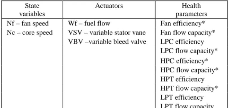
In this section the utility of the optimal tuner selection methodology is demonstrated by showing results from its application to the Commercial Modular Aero-Propulsion System Simulation (C-MAPSS), a NASA-developed high-bypass turbofan engine simulation (Ref. 9). C-MAPSS is a transient nonlinear aerothermodynamic engine model developed for controls and diagnostics research and develop-ment purposes. It has two state variables (fan and core speed), and three actuators (fuel flow, variable stator vanes (VSV), and a variable bleed valve (VBV)). C-MAPSS also has ten adjustable efficiency and flow capacity health parameters that enable the simulation of engine performance deterioration and module performance faults. The state variables, actuators, and health parameters are listed in Table 1. In this study, a simplified version of the C-MAPSS engine controller comprised of a fuel flow controller and variable geometry open-loop schedules is considered. While C-MAPSS does have control limit logic to prevent engine over speed and operating instabilities, that logic is not included here. The controller schedules fuel flow based on the error, ek, between
commanded and sensed fan speed. VBV and VSV actuators are open-loop scheduled based on sensed fan speed and sensed core speed, respectively. Collectively, fuel flow, VBV, and VSV commands form the vector of control inputs, uk,
provided as inputs to C-MAPSS. The C-MAPSS controller state variables and sensed feedback parameters are shown in Table 2.
For the purposes of this study, six sensed outputs and four unmeasured auxiliary outputs are defined. These parameters and their engineering units are listed in Table 3.
TABLE 1.—STATE VARIABLES, ACTUATORS, AND HEALTH PARAMETERS
State variables
Actuators Health
parameters
Nf – fan speed Wf – fuel flow Fan efficiency*
Nc – core speed VSV – variable stator vane Fan flow capacity*
VBV –variable bleed valve LPC efficiency
LPC flow capacity* HPC efficiency* HPC flow capacity* HPT efficiency HPT flow capacity* LPT efficiency LPT flow capacity *Health parameters applied as tuners in conventional estimation approach
TABLE 2.—CONTROLLER STATE VARIABLES AND SENSED FEEDBACKS
Controller state variables (xc)
Controller sensed feedbacks
xc(1) – fuel flow control state variable 1 yr – corrected fan speed
xc(2) – fuel flow control state variable 2 yo(1) – corrected fan speed
xc(3) – fuel flow control state variable 3 yo(2) – corrected core speed
xc(4) – VBV control state variable
xc(5) – VSV control state variable
TABLE 3.—SENSED OUTPUTS AND UNMEASURED AUXILIARY OUTPUTS Sensed outputs
(y)
Auxiliary parameters (z)
Nf – fan speed (rpm) T40 – Combustor exit temp. (○R)
Nc – core speed (rpm) T50 – LPT exit temperature (○R)
P24 – HPC inlet total pressure (psia) Fn – Net thrust (%)
T24 – HPC inlet total temp. (○R) SmLPC – LPC stall margin (%)
Ps30 – HPC exit static pressure (psia) T48 – Exhaust gas temperature (○R)
Case 1: Kalman Filter Point Design
As an initial evaluation, the optimal tuner selection metho-dology was applied to design a Kalman filter for application at a single closed-loop operating point. Here, model tuning parameters were selected to minimize a weighted sum of squared estimation errors (WSSEE) in the four auxiliary parameters listed in Table 3. To serve as a comparison, two additional Kalman filters were designed. These included a Kalman filter designed applying the conventional approach of selecting a subset of health parameters to form the model tuning vector, and a Kalman filter designed applying the open-loop optimal tuner selection approach presented in Refer-ence 6. The health parameters selected to serve as the elements of the tuner vector in the conventional design approach are denoted with an “*” in Table 1. They were selected through an exhaustive search that considered all possible combinations and determined the subset of six health parameters that
to C-MAPSS (a linear state space point model and the full nonlinear version) at steady-state closed-loop conditions at a provided the minimum WSSEE. All three designs were applied cruise operating point of 35K ft, 0.65 Mach, and a power lever angle (PLA) setting of 60°. In each case the engine was
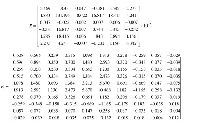
subjected to sensor measurement noise with covariance R
(with elements of the y vector in corrected engineering units, ordered as shown in Table 3), and health parameter deteriora-tion with covariance Ph (with elements of the h vector in
percent, ordered as shown in Table 1), defined as follows
5.469 1.830 0.047 0.381 1.585 2.273 1.830 131.195 0.022 16.817 18.415 4.241 0.047 0.022 0.002 0.007 0.006 0.007 0.381 16.817 0.007 3.744 1.843 0.232 1.585 18.415 0.006 1.843 7.894 1.156 2.273 4.241 0.007 0.232 1.156 6.342 R − − − − = − − − − 2 10− × 0.508 0.596 0.259 0.515 1.098 1.913 0.278 0.259 0.057 0.029 0.596 0.894 0.350 0.700 1.480 2.593 0.370 0.348 0.077 0.039 0.259 0.350 0.230 0.334 0.693 1.230 0.165 0.158 0.035 0.018 0.515 0.700 0.334 0.749 1.384 2.473 0.326 0.315 h P − − − − − − − = 0.070 0.035 1.098 1.480 0.693 1.384 3.213 5.670 0.691 0.669 0.147 0.075 1.913 2.593 1.230 2.473 5.670 10.468 1.182 1.165 0.258 0.132 0.278 0.370 0.165 0.326 0.691 1.182 0.206 0.179 0.037 0.019 0.259 0.348 0.158 0.315 0.669 1 − − − − − − − − − − − − − .165 0.179 0.183 0.035 0.018 0.057 0.077 0.035 0.070 0.147 0.258 0.037 0.035 0.018 0.004 0.029 0.039 0.018 0.035 0.075 0.132 0.019 0.018 0.004 0.012 − − − − − − − − − − − −
Note that the R and Ph matrices shown above contain
non-zero off diagonal elements. For R, this is due to the fact that the engine is operated closed-loop and parameter correction (Ref. 9) is applied. This results in non-zero covariance between each sensor measurement pair. To calculate R, a large simulated data set was generated by applying random noise to each sensor (i.e., the six sensors shown in Table 3 plus the inlet temperature and pressure sensors used for correction). The resulting covariance in the corrected sensor measurements yields R. The engine performance deterioration levels applied in this study are loosely based on historical aircraft engine data presented in Reference 10. This report shows that engine module deterioration occurs in a coupled fashion, resulting in some non-zero covariance between each health parameter pair. For this study, a routine was created to simulate random engine health parameter deterioration levels representative of the information shown in Reference 11. Based on a large simulated dataset generated by this routine, the health parameter covariance was calculated as Ph.
Table 4 shows a comparison of the theoretically predicted and experimentally obtained mean squared estimation errors for the three Kalman filter designs when applied to linear and nonlinear C-MAPSS operating in closed-loop. The experimen-tal results were obtained through a Monte Carlo simulation analysis in which the health parameters varied over a random
distribution in accordance with the covariance matrix, Ph
shown above. The test cases were concatenated to produce a single time history input that was provided to the C-MAPSS models. Each individual health parameter test case lasted 45 s. The experimental errors shown in Table 4 are based on the last 10.5 s of each 45 s test case. This allowed the engine model and the Kalman estimator to reach a quasi-steady-state operating condition prior to calculating the error. The corrected trim point values of T40, T50, Fn, and SmLPC are 2808 °R, 1222 °R, 26.5 percent, and 11.3 percent respectively. For the construc-tion of WSSEE, a weighting of 1.0 was applied to the T40 and T50 errors, and a weighting of 100.0 was applied to the Fn and SmLPC errors.
From Table 4 it can be seen that the mean squared estimation errors experimentally obtained from the linear model exhibit good agreement with the theoretically predicted errors. This result is encouraging as it validates the closed-loop optimal tuner selection methodology presented in this paper. It is also encouraging to find that the closed-loop optimal tuner selection approach provides superior estimation accuracy compared to the other two tuner selection approaches. A closer comparison of the closed-loop versus open-loop theoretical results reveals that the improvement offered by the closed-loop tuners is primarily due to a reduction in estimation variance. The mean squared estimation bias is nearly the same in both cases. This suggests
TABLE 4.—AUXILIARY PARAMETER MEAN SQUARED ESTIMATION ERRORS
Tuner vector Error T40 (°R) T50 (°R) Fn (%) Sm-LPC (%) WSSEE Subset of health parameters Theor. sqr. bias 20.48 0.69 0.003 0.031 24.51 Theor. variance 0.50 0.07 0.007 0.047 5.99 Theoretical 20.98 0.75 0.010 0.078 30.49 Exp. (linear) 20.16 0.78 0.010 0.075 29.43 Exp. (nonlinear) 24.52 1.39 0.012 0.197 46.73 Cruise optimal (open-loop) Theor. sqr. bias 1.58 0.52 0.001 0.014 3.60 Theor. variance 0.75 0.11 0.005 0.029 4.28 Theoretical 2.32 0.62 0.007 0.043 7.89 Exp. (linear) 2.26 0.64 0.007 0.044 7.92 Exp. (nonlinear) 4.49 1.19 0.007 0.163 22.73 Cruise optimal (closed-loop) Theor. sqr. bias 1.61 0.39 0.001 0.013 3.43 Theor. variance 0.36 0.07 0.000 0.002 0.64 Theoretical 1.97 0.45 0.002 0.015 4.06 Exp. (linear) 2.05 0.46 0.001 0.014 4.10 Exp. (nonlinear) 4.49 0.96 0.006 0.166 22.59
that the open-loop tuner selection approach, which is mathe-matically simpler and does not require access to detailed control design information, may be applied to provide comparable estimation accuracy, especially in applications that exhibit limited estimation variance. It is noted that the experimental estimation errors obtained based on nonlinear C-MAPSS are larger than those based on linear C-C-MAPSS. This is attributed to differences between the nonlinear plant model and the linear model that the Kalman filter is based upon. In particular, the SmLPC mean squared estimation error is significantly larger in the nonlinear case. This error, which has
a WSSEE weighting of 100, causes most of the increase
observed in WSSEE over the linear and theoretical results.
Case 2: Kalman filter Full-Envelope Design
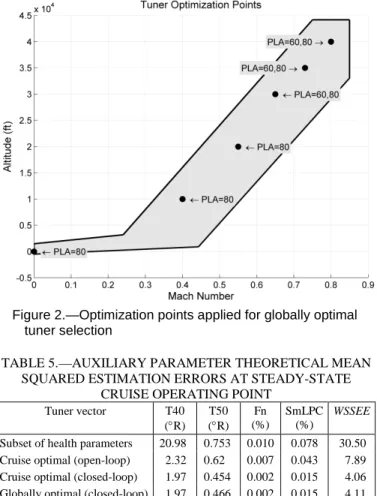
The previous case presented estimation results at a single operating point. However, to be practical the methodology must be applicable for constructing an estimator that can provide accurate estimation performance as the engine transitions throughout the flight envelope. As previously discussed, this can be performed by selecting a single globally optimal V* matrix for application within a piece-wise linear Kalman filter (PWLKF) design, enabling estimation through-out the entire operating envelope. The optimal iterative search routine was modified to sum the theoretical WSSEE results over multiple user-specified operating points. Through trial and error it was found that optimizing over a small number of operating points spanning the commonly encountered regions of the flight envelope provided reasonable estimation accuracy. To illustrate this technique, a single globally optimal
V* matrix was produced based on the nine engine operating points shown in Figure 2.
Table 5 shows the auxiliary parameter theoretical mean squared estimation errors obtained when applying the globally optimal V* matrix and tuner vector at the same closed-loop steady-state cruise operating condition used in Case 1. As a
Figure 2.—Optimization points applied for globally optimal tuner selection
TABLE 5.—AUXILIARY PARAMETER THEORETICAL MEAN SQUARED ESTIMATION ERRORS AT STEADY-STATE
CRUISE OPERATING POINT
Tuner vector T40 (°R) T50 (°R) Fn (%) SmLPC (%) WSSEE
Subset of health parameters 20.98 0.753 0.010 0.078 30.50
Cruise optimal (open-loop) 2.32 0.62 0.007 0.043 7.89
Cruise optimal (closed-loop) 1.97 0.454 0.002 0.015 4.06
Globally optimal (closed-loop) 1.97 0.466 0.002 0.015 4.11
comparison, the theoretical mean squared estimation errors based on the three model tuner vectors evaluated in Case 1 are also shown. The encouraging result is that application of the globally optimal tuner vector does not result in a significant loss in estimation accuracy. In fact, the WSSEE of the globally optimal tuner vector is only 1.2 percent larger than that of the tuner vector optimally selected for the given cruise operating point. Even more impressive is the fact that the evaluated cruise point is not one of the nine points used to determine the globally optimal V*.
As an additional comparison, the average theoretical estima-tion accuracy provided by the subset of health parameters, cruise optimal closed-loop, and globally optimal closed-loop tuner vectors was evaluated at 2000 operating points spanning the engine operating envelope. For this evaluation, separate Kalman filter point designs were constructed at each of the 2000 operating points. These results are shown in Table 6, along with the standard deviation in the results (shown in parentheses). Here it can be observed that the Kalman filter design that applies the globally optimal tuner vector provides a 4.2 percent reduction in WSSEE compared to the cruise optimal tuner vector. Furthermore, the standard deviation in all squared estimation errors is relatively small, demonstrating little variance in the estimation error as the operating point is changed. These results are highly encouraging as they suggest that a fixed tuner vector, which is near optimal over a large
TABLE 6.—AUXILIARY PARAMETER THEORETICAL MEAN SQUARED ESTIMATION ERRORS (AND
STANDARD DEVIATION) AVERAGED OVER 2000 STEADY-STATE OPERATING POINTS
Tuner vector T40 (°R) T50 (°R) Fn (%) SmLPC (%) WSSEE Subset of health parameters 20.03 0.762 0.012 0.054 27.36 (1.94) (0.155) (0.005) (0.016) Cruise optimal (closed-loop) 1.90 0.711 0.003 0.014 4.27 (0.16) (0.531) (0.002) (0.003) Globally optimal (closed-loop) 1.90 0.634 0.003 0.013 4.09 (0.15) (0.298) (0.001) (0.002)
region of the flight envelope, can be found. However, additional evaluation is warranted to demonstrate that a globally optimal tuner vector can be generated and applied to other engine models in addition to C-MAPSS.
Case 3: Kalman Filter Design Considerations
For Transient Operating Conditions
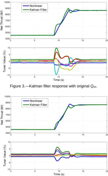
The optimal tuner selection strategy presented in this paper is designed to minimize the mean squared estimation error under steady-state operating conditions. However, it does not necessarily provide the desired accuracy when the engine is undergoing a transient. To illustrate this refer to Figure 3. The top half of this figure shows a comparison of nonlinear C-MAPSS net thrust versus a PWLKF estimate of net thrust as the engine undergoes a power transient at a cruise condition (35K ft, 0.65 Mach). The lower half of the figure shows the corresponding variation in the estimates of the tuning parameters, q, produced by the Kalman filter. In this example, nonlinear C-MAPSS is a nominal (non-deteriorated) engine, whereas the PWLKF is based on a fleet average (50 percent deteriorated) engine. Before and after the transient operating period, the actual and estimated net thrust exhibit good agreement. However, during the transient the estimate produced by the Kalman filter responds more rapidly than the actual thrust; consequently the estimate is not as accurate. It can also be observed that the tuner estimates undergo signifi-cant variations during the transient.
A design step that can be taken to adjust the dynamic re-sponse of the Kalman filter estimates is to modify the specified process noise covariance matrix, Qxh. Specifying
smaller magnitude values will slow the dynamic response of the Kalman filter estimates. To illustrate this, the Qxh matrix
was divided by 1106, and the optimal tuner selection process was repeated. The identified vector of tuning parameters was then applied to design a new Kalman filter. The response of the new Kalman filter to the same power transient is shown in Figure 4. Here it can be observed that the estimation accuracy during the transient is improved, and the amount of variation in the tuning parameters during the transient is also reduced.
Figure 3.—Kalman filter response with original Qxh.
Figure 4.—Kalman filter response with adjusted Qxh.
Conclusions
A systematic approach to model tuning parameter selection for on-line Kalman filter based parameter estimation under closed-loop operating conditions has been presented, along with design considerations for applying the approach. This technique is specifically for the underdetermined parameter estimation problem where there are fewer sensor measure-ments than unknown health parameters that impact system outputs. The approach creates and applies a linear transforma-tion matrix, V*, to select a vector of tuning parameters that are a linear combination of all health parameters. The tuning parameter vector is selected to be of low enough dimension to be estimated, while minimizing the mean-squared error of Kalman filter estimates. Evaluations based on an aircraft
engine linear point model demonstrate that the theoretically predicted and experimentally obtained estimation errors exhibit good agreement, thus confirming the theory that the tuner selection methodology is based upon. The technique was also found to provide acceptable estimation results when applied to a nonlinear aircraft turbofan engine simulation, although, as expected, some loss in estimation accuracy is incurred compared to the linear evaluation. Additionally, a technique for selecting a single globally optimal V* matrix applicable throughout an engine’s operating envelope has been demonstrated. This is necessary to enable interpolation between operating points within a piece-wise linear design implementation. Theoretical evaluation results using an
aircraft engine model showed that the application of a single globally optimal V* matrix results in only a 1.2 percent increase in mean squared estimation error compared to the implementation of an optimal V* matrix at a cruise operating point. While encouraging, additional evaluation is warranted to determine if this holds when the technique is applied to different engine operating points and different engine models. Finally, it was also shown that, as in a conventional Kalman filter implementation, the system designer can adjust the dynamic response of the Kalman filter estimates by adjusting the specified state vector process noise covariance matrix used in the filter design.
Appendix: Derivation of Kalman Filter Mean Squared
Estimation Error Under Closed-Loop Operating Conditions
This appendix provides a derivation of the Kalman filter mean squared estimation error at a closed-loop steady-state operating point. This information is used in the iterative search for an optimal V* matrix described in the paper. This appendix will first derive the control inputs, system outputs, and Kalman filter estimates under steady-state conditions. Next, the Kalman filter mean squared estimation error, which is comprised of a mean squared bias and a mean variance, will be derived.
System Under Steady-State Conditions
For the linear system operating at the trim point under steady-state conditions rk = 0 and xk+1=xk =xss
. We can leverage this information to write the x, y, and z equations as a function of h
(
)
(
)
(
)
1 1 1 ss ss ss ss ss ss ss ss ss x Ax Lh x I A Lh y Cx Mh y C I A L M h z Fx Nh z F I A L N h − − − = + = − = + = − + = + = − + (A.1)The steady-state actuator commands, uss, and the steady-state
state vector, xss, can also be written as functions of h, so from
Eqs. (5) and (A.1)
(
)
[
]
[
]
(
)
1 1 0 0 0 0 ss ss ss c ss c x ss ss x u C x C I A Lh x I x I I A Lh − − = = − = = − (A.2)Steady-state Kalman filter estimates can also be written as a function of h. To make this derivation we will begin by rewriting the a priori and a posteriori Kalman filter equations previously given in Eqs. (19) and (20) as follows
a priori equations
(
)
(
)
(
)
1 , , 1 1 , , 1 1 , 1 1 ˆ 1 , , 1 1 , 1 1 1 , , 1 ˆ ˆ ˆ ˆ ˆ ˆ ˆ ( ˆ ) ˆ ˆ k xq k xq xq k xq k xq k xq xq k k xq xq k k x xq k xq k xq xq k xq k xq xq k k xq k xq k xq xq xq k xq x A x B u x A x K y C x Du B u x A x A K y C x Du B u x A I K C x A K + − − + − − − − − − ∞ − − − − − − − − ∞ − − − − − − ∞ − ∞ = + = + − − + = + − − + = − + 1 1 k xq xq k y B A K D u − ∞ − − (A.3) a posteriori equations(
)
(
)
(
)
(
)
[
]
, , , , , , , ˆ ˆ ˆ ˆ ˆ ˆ ˆ xq k xq k k xq xq k k xq k xq xq k k k k xq k xq xq k k x x K y C x Du x I K C x K y Du y x I K C x K K D u + − − ∞ + − ∞ ∞ + − ∞ ∞ ∞ = + − − = − + − = − + − (A.4)Next, the following expected value properties at steady-state operating conditions are defined
1 1 , , 1 , ˆ ˆ ˆ k k ss k k ss xq k xq k xq ss E y E y y E u E u u E x E x x − − − − − − = = = = = = (A.5)
Substituting (A.5) into (A.3) allows the a priori Kalman filter equation under steady-state conditions to be written as
(
)
, , ˆxq ss xq xq ˆxq ss ss xq xq xq ss x A I K C x y A K B A K D u − − ∞ ∞ ∞ = − + − (A.6)Then, substituting Eqs. (A.1) and (A.2) into (A.6), the steady-state Kalman filter a priori equation can be written as a function of h.
(
)
(
)
(
)
(
)
(
)
(
)
(
)
1 , , 1 1 1 , 1 ˆ ˆ 0 ˆ 0 xq ss xq xq xq ss xq xq xq c xq ss xq xq xq xq xq c C I A L M x A I K C x A K B A K D h C I A L C I A L M x I A I K C A K B A K D h C I A L − − − ∞ ∞ ∞ − − − − ∞ ∞ ∞ − − + = − + − − − + = − − − − (A.7)Next, proceed to the a posteriori Kalman filter equations, which can also be written as a function of h
(
)
[
]
(
)
(
(
)
)
( )
( )
[
]
( )
( )
, , 1 1 1 , 1 1 , ˆ ˆ ˆ 0 0 ˆ ss xq ss xq xq ss ss xq ss xq xq xq xq xq xq c c xq ss y x I K C x K K D u C I A L M C I A L M x I K C I A I K C A K B A K D h K K D h C I A L C I A L x I K + − ∞ ∞ ∞ − − − + ∞ ∞ ∞ ∞ ∞ ∞ − − + ∞ = − + − − + − + = − − − − + − − − = − (
)
(
(
)
)
[
]
( )
( )
1 1 1 , 0 ˆ xq xq xq xq xq xq xq c G xq ss xq C I A L M C I A I K C A K B A K D K K D h C I A L x G h − − ∞ ∞ ∞ ∞ ∞ − + − + − − − + − − = (A.8)Steady-State Mean Squared Estimation Error
Using Eqs. (21), (A.8), and (A.2), the steady-state mean estimation error bias is given as
[
]
(
)
[
]
(
)
, , , , , , , 1 *† ˆ 1 *† ˆ ˆ 0 0 0 0 0 0 xq ss xh ss xh ss xh ss xh k xh k xh ss xh ss ss xq x x xq G ss s x x E x x x x h I I I A L G h h V I I I I A L G h V I x h + + + − − = = − = − − = − − = − = xh s G h = (A.9)The steady-state auxiliary parameter estimation error bias can also be derived using Eqs. (15), (A.1), and (A.8)
(
)
*† , 1 *† ˆ ˆ ˆ z ss k k ss ss xq ss ss xq G z z E z z z z F NV x z F NV G F I A L N h G h + − = − = − = − = − − + = (A.10)Mean Squared Estimation Error Bias
The average sum of squared estimation error biases across a fleet of engines can be calculated from Eqs. (A.9) and (A.10) as follows
{
}
{
}
{
}
2 , , , , , h T T xh fleet xh ss xh ss xh ss xh ss T T xh xh T T xh xh P T xh h xh x E x x E tr x x E tr G hh G tr G E hh G tr G P G ≡ = = = ⋅ = (A.11){ }
{
}
{
}
2 h T T fleet ss ss ss ss T T z z T T z z P T z h z z E z z E tr z z E tr G hh G tr G E hh G tr G P G ≡ = = = ⋅ = (A.12)where tr{●} represents the trace (sum of the diagonal elements) of the matrix.
Estimation Error Variance
Next, derivations are presented for the covariance matrix of the augmented state estimate and of the auxiliary parameter
estimate, ˆ ˆ ,
xh k
P and Pˆ,z krespectively. These matrices will each be calculated as a function of the reduced-order state vector estimation covariance matrix,Pˆ ˆ,xq k, which is defined as
(
)(
)
, , ˆ ˆ, ˆ , ˆ , ˆ , ˆ , T xq k xq k T xq k xq k xq k xq k xq k P E x+ E x+ x+ E x+ ε ε = − − (A.13)where the vector εxq,k is defined as the residual between xˆxq k,
+
at time k and its expected value. Since E xˆxq k+, =xˆxq ss+, , εxq,k can
be obtained by subtracting Eq. (A.8) from Eq. (20)
(
)
[
]
(
)
[
]
(
)
(
)
, , , , , , , , , ˆ , ˆ , 1 1 ˆ ˆ ˆ ˆ ˆ ˆ ˆ ˆ xq k xq ss xq k xq k xq k xq k xq k xq ss k xq xq k k x ss xq xq ss ss x xq xq xq k xq k x x E x x x y I K C x K K D u y I K C x K K D u I K C A x B u + + − + + + + − ∞ ∞ ∞ − ∞ ∞ ∞ + ∞ − − ε = − = − = − + − − − + − = − + [
]
(
)
(
)
[
]
(
)
(
)
(
)
, , , ˆ , ˆ ˆ , 1 , ˆ ˆ ˆ xq k xq ss xq ss k k x ss xq xq xq ss xq ss ss x x xq xq xq k xq ss k xq xq y K K D u y I K C A x B u K K D u I K C A x x y y K K D I K C B + − + ∞ ∞ + ∞ ∞ ∞ + + ∞ − ∞ ∞ ∞ + − − − + + − = − − − + − − 1 ss k ss k ss u u u − u − − (A.14)While the actuators will exhibit some variance due to mea-surement noise in the control feedback sensors, their contribu-tion to the overall estimacontribu-tion variance is not as large as that of the sensor measurements. Therefore, to help simplify this derivation we will assume that the actuator commands are held
constant at uss (they have no variance). With this simplifying
assumption uk = uk+1 = uss, allowing Eq. (A.14) to reduce to
(
)
(
)
(
)
, ˆ , 1 ˆ , xq k I K Cxq Axq xxq k xxq ss K yk yss + + ∞ − ∞ ε = − − + − (A.15)Next, we can substitute Eq. (A.15) into Eq. (A.13) and manipulate to produce the following Riccati equation:
ˆ ˆ, ˆ ˆ, T xq xq xq xq xq xq xq k xq k T P A K C A P A K C A K RK ∞ ∞ ∞ ∞ = − − + (A.16)
The above Riccati equation can be solved to calculate the covariance in the state and health parameters estimates, or in the auxiliary parameter estimates:
ˆ ˆ ˆ, ˆ, *† *† 0 0 0 0 T xq k xh k I I P P V V = (A.17) *† *† ˆ ˆ ˆ, , T z k xq k P = F NV P F NV (A.18)
Sum of Squared Estimation Errors
Once equations (A.11), (A.12), (A.17), and (A.18) are obtained, they may be used to analytically calculate the mean sum of squared estimation errors over all engines by combin-ing the respective mean squared estimation error bias and estimation variance information. The mean sum of squared estimation errors of the augmented state vector, ˆ
ˆ,
x h
SSEE
, and the mean sum of squared estimation errors of the auxiliary parameter vector, ˆ z SSEE , become{ }
{
}
{ }
{
}
2 ˆ , ˆ ˆ, ˆ, ˆ ˆ , 2 ˆ ˆ, ˆ, xh fleet x h xh k T xh h xh xh k z fleet z k T z h z z k SSEE x tr P tr G P G P SSEE z tr P tr G P G P = + = + = + = + (A.19)A weighting, Wz, can be applied to calculate a “weighted” sum
of auxiliary parameter squared estimation errors given as
{
}
ˆ ˆ,
T
z z z h z z k
WSSEE =tr W G P G +P (A.20)
The SSEE or WSSEE equation, given in Eqs. (A.19) and (A.20) respectively, can be directly applied within the iterative search for an optimal V* matrix as denoted in Eq. (22).
References
1. Luppold, R.H. Roman, J.R., Gallops, G.W., Kerr, L.J., (1989), “Estimating In-Flight Engine Performance Var-iations Using Kalman Filter Concepts,” AIAA-89-2584, AIAA 25th Joint Propulsion Conference.
2. Volponi, A., (2008), “Enhanced Self-Tuning On-Board Real-Time Model (eSTORM) for Aircraft Engine Per-formance Health Tracking,” NASA/CR—2008-215272. 3. Kumar, A., Viassolo, D., (2008), “Model-Based Fault
Tolerant Control,” NASA/CR—2008-215273.
4. España, M.D., (1994), “Sensor Biases Effect on the Estimation Algorithm for Performance-Seeking Control-lers,” J. Propulsion and Power, 10, pp. 527-532. 5. Litt, J.S., (2008), “An Optimal Orthogonal
Decomposi-tion Method for Kalman Filter-Based Turbofan Engine Thrust Estimation,” Journal of Engineering for Gas
Tur-bines and Power, Vol. 130 / 011601-1.
6. Simon, D.L., Garg, S., (2010), “Optimal Tuner Selection for Kalman Filter-Based Aircraft Engine Performance Estimation,” Journal of Engineering for Gas Turbines
and Power, Vol. 132 / 0231601-1.
7. Simon, D., (2006), Optimal State Estimation, Kalman,
H∞, and Nonlinear Approaches, John Wiley & Sons,
Inc., Hoboken, NJ.
8. Kwakernaak, H., Sivan, R., (1972), Linear Optimal
Control Systems, John Wiley & Sons, Inc., New York,
NY.
9. DeCastro, J.A., Litt, J.S., Frederick, D.K., “A Modular Aero-Propulsion System Simulation of a Large Com-mercial Aircraft Engine,” AIAA-2008-4579, 44th AIAA/ASME/SAE/ASEE Joint Propulsion Conference & Exhibit, Hartford, CT, July 21-23, 2008.
10. Volponi, A.J., 1999, “Gas Turbine Parameter Correc-tions,” Journal of Engineering for Gas Turbines and
Power, Vol. 121, pp. 613–621.
11. Sallee, G.P., (1978) “Performance Deterioration Based on Existing (Historical) Data – JT9D Jet Engine Diag-nostics Program,” NASA Contractor Report CR-135448, United Technologies Corporation, Pratt & Whitney Air-craft Group Report PWA-5512-21.