Università degli Studi di Padova
Dipartimento di Ingegneria dell’Informazione
Unlabeled pattern management through
Semi-Supervised classification techniques
Relatore: Prof. Loris Nanni
Laureando: Giordano Segato
Corso di laurea magistrale in ingegneria informatica
Data di laurea: 14/10/2014
Summary
The purpose of this thesis work is to analyze different state-of-art semi-supervised learning
algorithms that has been proposed in last years. In semi-supervised learning, unlabeled data are used together with labeled data to provide better performance in the classification process.
In the experimental phase, the implemented algorithms have been applied to various datasets usually tested in the academic research. Used datasets are real-world datasets available at UCI (University of California, Irvine) website.
A second phase of the experiments consists in the fusion and combination of the analyzed algorithms in order to obtain a classification algorithm with good performance in each tested dataset. This goal represents the implementation of an algorithm with robustness properties, which can be used in a dataset independently from its nature, in a general purpose classifier.
Index
Introduction ... 1
Machine Learning ... 5
2.1
Classification ... 6
2.2
Support Vector Machine ... 7
2.2.1 Linear SVM: separable case ... 8
2.2.2 Linear SVM: not separable case ... 12
2.2.3 Non-linear SVM ... 13
2.2.4 libSVM ... 14
2.2.5
One-vs-all
approach ... 16
2.3
Semi-Supervised Learning ... 17
2.3.1 Assumption for Semi-Supervised Learning ... 20
2.3.2 Semi-supervised algorithms ... 22
2.3.3 Self-training ... 23
2.3.4 Co-training ... 25
2.3.5 Help training ... 26
2.3.6 Adaptive bootstrap ... 27
2.4
Risks of Semi-Supervised Learning ... 28
2.4.1 Methodological Considerations ... 29
2.4.2 Active Learning ... 29
Proposed system... 31
3.1 Reference Articles ... 31
3.1.1 DCPE co-training for classification ... 31
3.1.2 Using clustering analysis to improve semi-supervised classification .... 36
3.1.3 A semi-supervised feature ranking method with ensemble learning .... 41
3.1.4 Single Classifier-based Multiple Classification Scheme ... 48
Experimental results ... 59
4.1
Used configuration framework for data ... 60
4.1.1 Validation phase ... 61
4.2
Datasets ... 62
4.3.1 Initial Datasets Elaboration ... 65
4.3.2 Data Normalization ... 66
4.3.2 Considerations and details about datasets ... 67
4.4 Tests schemas ... 69
4.4.1
Test 1 ... 70
4.4.2
Test 2 ... 70
4.4.3
Test 3 ... 73
4.4.4
Test 4 ... 83
4.4.5
Test 5 ... 86
Conclusions ... 89
Bibliography ... 93
1
Chapter 1
Introduction
In the current Information Age there has been an extraordinary growth of data that have been generated and stored in millions of data structures. Consequently, the availability of very large volumes of data has created a problem of how to extract useful information.
Traditionally, data analysis techniques that have been used for such tasks include regression analysis, cluster analysis, numerical taxonomy, multidimensional analysis, other multivariate statistical methods, stochastic models, time series analysis, non-linear estimation techniques, and others. These techniques have been widely used for solving many practical problems.
Statistical data analysis is primarily oriented toward the extraction of quantitative data characteristics, and as such has inherent limitations. For example, a statistical analysis can determine average and correlations between variables in data, but it cannot characterize the dependencies at an abstract and conceptual level, providing a causal explanation of the reasons why these dependencies exist.
Moreover, the statistical techniques can determine the central tendency and variance of given factors, while regression analysis can fit a curve to a set of samples. However, these techniques can’t produce a qualitative description of the dataset structure and determine the dependences not explicitly provided in the data.
Methods based on numerical analysis can create a classification of samples and specify a numerical similarity among the samples assembled into the same or different categories. This approach however can’t build qualitative description of the reasons behind class assignment.
2
In summary, traditional data analysis techniques facilitate useful data interpretations and can help to generate important insights into the processes behind the data. In efforts to satisfy the growing need for new data analysis tools that will overcome the limitations of traditional statistical analysis, researchers have turned to ideas and methods developed in machine learning.
The last decade has experienced a revolution in terms of information availability and exchange. The World Wide Web and the amount of produced data is growing at an exponential rate.
Moreover many businesses and organizations have begun to collect data regarding their own operations and market opportunities on a large scale. An important challenge consists in the “extraction” of useful information from the provided amount of data. Beyond the immediate purpose of tracking or archiving the activities of an organization, the collected data can sometimes represent an important resourcefor strategic planning and decisions. Research and development in this area are often referred to as data mining and knowledge discovery in databases (KDD) [14].
The goal of data mining algorithms is to extract useful information from large data archives. Reached information can be obtained:
Directly, in the form of “knowledge” characterizing the relations between the variables of interest.
Indirectly, as functions that allow to predict, classify, or represent information in the distribution of the data.
In the field of data mining and knowledge discovery, new techniques and algorithms have been developed to deal with the computational complexity deriving from the large amount of data. However the large availability of data can provide good performance in the classification, also considering unlabeled data in the training phase, using techniques called semi-supervise learning [2] [10].
3
Many different approaches and algorithms have been proposed. For example techniques oriented to obtain robustness property (especially in the case of noisy datasets), or feature selection techniques which provide good performance with high-dimensional datasets [8].
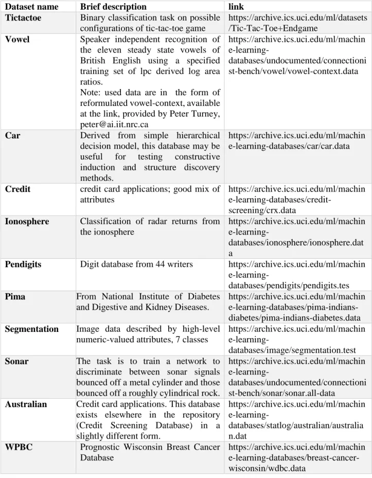
In this thesis work, four algorithms have been implemented and analyzed, Analyzed methods have been published in papers distributed in the last years [6] [7] [8] [9]. Then the algorithms have been tested on various datasets available online in the UCI website: https://archive.ics.uci.edu/ml/machine-learning-databases. A detailed description of datasets is illustrated in sections 4.2 and 4.3.
The implemented algorithms regard different techniques and are described in the relative reference articles:
Classifier which uses a generated set of artificial samples [6]
Advanced technique based on semi-supervised learning [7]
A semi-supervised feature ranking method [8]
Using clustering analysis to improve semi-supervised classification [9]
These different approaches are described in section 3.
In section 4, the experiments that have been done are explained and the dataset division (labeled, unlabeled, validation data) is illustrated.
5
Chapter 2
Machine Learning
Machine Learning is the discipline that study algorithms which allow to identify patterns in data. Over the past years Machine Learning has become one of the most important fields of information technology. With the ever increasing amounts of available data, there are good reasons to believe that smart data analysis will become even more pervasive as a necessary component of the technological progress.
Usually, major machine learning problems can be divided in three groups of problems: Association analysis, clustering and classification.
Association Analysis: this task consists in searching for patterns that describe strong associations among the features. The discovered patterns are typically represented in the form of implication rules between feature subsets. Because of the exponential size of its search space, the goal of association analysis is to extract the most interesting patterns in an efficient manner. Useful applications of association analysis include finding groups of genes that have related functionality, identifying web pages that are accessed together, or understanding the relationships between different elements of Earth’s climate system.
Classification: it consists in the construction of a model that allows to classify records assigning them a label. The base form of classification has two phases: a learning phase which create a model
6
on a dataset of already classified data, and a test phase which is used to test the obtained model and get a measure of performance. Test phase tests the classifier built in training phase on a test set; the classifier assigns to any record a label and then resulting labels are compared with real classes and an accuracy measure is calculated.
Clustering: itis the problem of dividing data in clusters, based on the attributes values. It can be used for group newspaper articles or website and can be similar to classification for some aspects.
In this thesis will be used classification techniques prevalently based on the Support Vector Machine (SVM) classifier, so in the next this argument will be examined in depth.
2.1 Classification
Classification is the task of assigning a label to an input object. It’s a very common problem and it has many different real-world applications. Examples include detecting spam email messages based on the message header and content, categorizing cells as malignant or the classification of galaxies based upon their shape.
To solve the classification problem, different learning algorithms have been proposed and each algorithm has advantage and disadvantage. Most diffused algorithms are:
Decision Tree: it is very simple to implement and it has good time performance. However accuracy is not very high and there are more convenient learning algorithms. It consists in the constructions of a decision tree by progressively splitting the features values. This technique also provides in output an intuitive tree diagram and so it is also useful to understand the internal data structure [5].
7
Bayesian Classifier[24]: it classifies a record estimating the probability that the sample belongs to each class and choosing the most probable class. However, in a dataset every sample is almost unique, and so it’s impossible to directly estimate the needed probability. For this reason the Bayes theorem is used. This theorem provides the method to estimate the posterior probability 𝑃(𝑌|𝑿) (probability of a class conditioned to the sample’s value) in terms of the prior probability 𝑃(𝑌), the class conditional probability 𝑃(𝑿|𝑌) and the evidence 𝑃(𝑿):
𝑃(𝑌|𝑿) =𝑃(𝑿|𝑌) × 𝑃(𝑌)
𝑃(𝑿) (2.1)
Artificial Neural Networks: it’s a network that can ‘learn’ a model of classification, changing its configuration. It is very used in machine learning. Analogous to human brain structure, an Artificial Neural Network is composed of an interconnected assembly of nodes and direct links [23].
Support Vector Machine: Support vector machine (SVM) is a technique of automatic learning for the classification of data. It is based on the idea of dividing the features space using a function that allows to separate the different classes [25].
2.2 Support Vector Machine
Support vector machine (SVM) is a technique of automatic learning for the classification of data. The idea is to divide the features space using a function that allows to separate the different classes. Support Vector Machine is one of the most used techniques of classification because of its good performance in terms of accuracy and time consumption. This technique has shown promising empirical results in many practical applications, from handwritten digit recognition to text categorization. SVM also works very well with high-dimensional data and avoids the curse of
8
dimensionality problem. Another unique aspect of this approach is that it represents the decision boundary using a subset of the training samples, known as the support vectors.
There exists different kind of SVM. Considering linearity, SVM can be divided in linear and non-linear. Non-linear SVM is reduced to linear case using a kernel function that allows to create a space with more dimensions than the number of the features, so the mathematical techniquesof linear case can be applied to the extended space.
Moreover, considering data distribution, linear SVM can be divided in two cases: linearly separable and not linearly separable. In linearly separable case there exists a boundary that allows to divide the feature space among different classes, while this is not possible in not separable case, where is needed to use a soft margin approach (where the decision boundary is built considering the possibility of misclassifying records in training phase). This approach is useful also in separable case, in order to avoid overfitting.
In the next we analyze the case of two classes. Then, when classes are more than two, there are algorithms that allow to reduce the problem to the two classes case. In the experiments of chapter 4, the one versus all approach is used.
2.2.1 Linear SVM: separable case
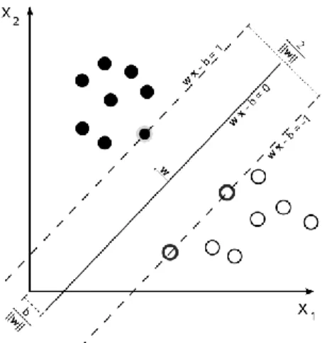
The base case of SVM is linear SVM in a separable problem, where the SVM is the optimal boundary that maximizes the distance between the groups of records of the same class. The goal is to found a function that describes the decision boundary in the space of features. In this case such boundary exists for hypothesis, so is used a hard margin approach that searches the optimal hyperplane dividing the dataset.
9
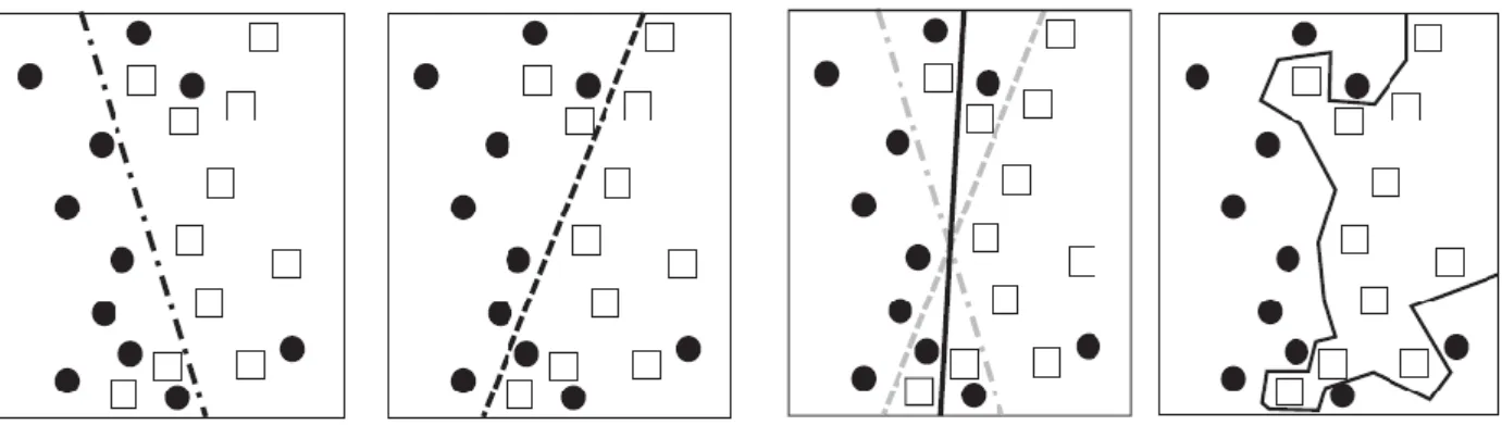
Firstly, a margin is defined as shown in Figure 2.1; the margin represents the distance from boundary to the nearest element of each class. Then, it’s formalized an optimization problem on the margin length, which will be solved using Lagrange multiplier method.
Consider a binary classification problem consisting of 𝑁 training samples. Each sample is denoted by a tuple (𝑥𝑖, 𝑦𝑖) where 𝑥𝑖 = (𝑥𝑖,1, 𝑥𝑖,2, … , 𝑥𝑖,𝑑) corresponds to the attribute set for the 𝑖 − 𝑡ℎ sample. Using conventionally {−1,1} as classes, the decision boundary will have the form:
𝑊 ∙ 𝑥 + 𝑏 = 0 (2.2)
Where 𝑤 and 𝑏 are the parameters which have to be determined solving the optimization problem. The first step consists in determine the coefficients 𝑊 and 𝑏 of (2.2). For every record, the following conditions must be verified:
𝑊 ∙ 𝑥𝑖 + 𝑏 ≥ 1 𝑖𝑓 𝑦𝑖 = 1 (2.3)
𝑊 ∙ 𝑥𝑖 + 𝑏 ≤ −1 𝑖𝑓 𝑦𝑖 = −1 These conditions can be summarized in the following:
𝑦𝑖(𝑤 ∙ 𝑥𝑖+ 𝑏) ≥ 1 𝑖 = 1,2, … , 𝑁 (2.4)
As in Figure 2.1, the margin in separable case is defined as the minimum distance between elements of different classes (in the figure it is represented the case of a space of two features, but it is the analog of the case with more features). The nearest elements to the boundary are called support vectors of the relative class. Considering two points of different class 𝑥1 and 𝑥2, the distance between the hyperplanes passing on the support vectors is determined as follow. Initially the parameters 𝑊 and 𝑏 are scaled in order to obtain hyperplanes passing on the support vectors described by the following equations:
𝑊 ∙ 𝑥1+ 𝑏 = 1 (2.5)
𝑊 ∙ 𝑥2+ 𝑏 = −1
So
10
‖𝑊‖ ∙ 𝑑 = 2
𝑑 = 2
‖𝑤‖
Where 𝑑 is the distance between hyperplanes passing on the support vectors.
To solve the problem of optimization of the separation, we need to maximize the margin, which means to minimize the function:
𝐹(𝑥) =‖𝑤‖22 (2.7)
Considering the boundaries (2.3). We get the following optimization problem:
𝑂𝑏𝑗𝑒𝑐𝑡𝑖𝑣𝑒 𝑓𝑢𝑛𝑐𝑡𝑖𝑜𝑛: min 𝑤
‖𝑤‖2
2 (2.8)
𝐶𝑜𝑛𝑠𝑡𝑟𝑎𝑖𝑛𝑡𝑠: 𝑦𝑖(𝑤 ∙ 𝑥𝑖+ 𝑏) ≥ 1 𝑖 = 1,2, … 𝑁
11
This problem is a convex optimization problem, because the objective function is quadratic. It can be solved with Lagrange multipliers method.
Intuitively the process to use the Lagrange multipliers is the following:
1) We construct a Lagrangian function, which takes into account the boundaries:
𝐿𝑝 =
1
2‖𝑊‖2− ∑ 𝜆𝑖∙ (𝑦𝑖(𝑤 ∙ 𝑥𝑖+ 𝑏) − 1) (2.9)
𝑁
𝑖=1
Where 𝜆𝑖 are the Lagrange multipliers and must be determined
2) We can hypnotize 𝜆𝑖 ≥ 0 , in fact every solution with negative Lagrange multipliers can only increase the objective function
3) We impose the derivatives of 𝐿𝑃respect to 𝑤 and 𝑏 equal to zero:
𝜕𝐿𝑃 𝜕𝑤 = 0 ⇒ 𝑤 = ∑ λi⋅ yi∙ xi (2.10) 𝑁 𝑖=1 𝜕𝐿𝑝 𝜕𝑏 = 0 ⇒ 𝑤 = ∑ λi∙ yi = 0 𝑁 𝑖=1
4) The set of inequality in the optimization problem can be replaced by equality, thanks to the fact that the Lagrange multiplier are greater than zero. These conditions are also called the Karush-Kun-Tucker conditions (KKT):
𝜆𝑖 ≥ 0 (2.11)
𝜆𝑖(𝑦𝑖(𝑊 ∙ 𝑥𝑖 + 𝑏) − 1) = 0
5) The problem is simplified considering the dual problem. The Lagrangian is transformed into a function of the Lagrange multipliers only.
When the problem will be solved, only the support vectors will have a value of 𝜆𝑖 ≠ 0 and that will be used also to determine decision value and probability estimation in practical implementation.
12
2.2.2 Linear SVM: not separable case
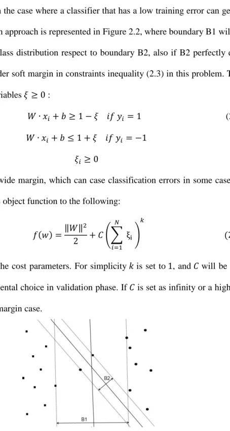
In not separable case we can’t define an optimization problem with a boundary that is valid for all records in the features space. So it’s used a soft margin approach. Soft margin approach can be applied also to avoid overfittng, in the case where a classifier that has a low training error can generate low final accuracy. Soft margin approach is represented in Figure 2.2, where boundary B1 will provide a better description of the class distribution respect to boundary B2, also if B2 perfectly divides the dataset. We need to consider soft margin in constraints inequality (2.3) in this problem. This can be done introducing slack variables 𝜉 ≥ 0 :
𝑊 ∙ 𝑥𝑖 + 𝑏 ≥ 1 − 𝜉 𝑖𝑓 𝑦𝑖 = 1 (2.12)
𝑊 ∙ 𝑥𝑖+ 𝑏 ≤ 1 + 𝜉 𝑖𝑓 𝑦𝑖 = −1
𝜉𝑖 ≥ 0
This allows to consider a wide margin, which can case classification errors in some case. To avoid this we need to modify the object function to the following:
𝑓(𝑤) =‖𝑊‖2 2 + 𝐶 (∑ ξi 𝑁 𝑖=1 ) 𝑘 (2.13)
Where 𝐶 and 𝑘 represent the cost parameters. For simplicity 𝑘 is set to 1, and 𝐶 will be chosen for example as better experimental choice in validation phase. If 𝐶 is set as infinity or a high value, the situation will be the hard margin case.
13
2.2.3 Non-linear SVM
Non-linear SVM takes into account the case in which the boundary function used to divide the feature space is not linear. This can generate a better accuracy, but is more computationally expensive than the linear SVM. To solve the problem of determine a non-linear boundary, the data are transformed from the original coordinate space in 𝑋 into a new space 𝜙(𝑥), so that a linear boundary can be used to separate the instances in the new space. After the transformation of the space of features, the previous strategy can be apply to define a classification model.
After the transformation, the linear problem will be the following:
𝑂𝑏𝑗𝑒𝑐𝑡𝑖𝑣𝑒 𝑓𝑢𝑛𝑐𝑡𝑖𝑜𝑛: min 𝑊
‖𝑊‖2
2 (2.14)
𝐶𝑜𝑛𝑠𝑡𝑟𝑎𝑖𝑛𝑡𝑠: 𝑦𝑖(𝑊 ∙ 𝜙(𝑥) + 𝑏) ≥ 1 𝑖 = 1,2, … 𝑁
Which is similar to problem (2.8) except for the substitution of 𝑥 by 𝜙(𝑥). The dual Lagrangian problem has the following form:
𝐿𝐷 = ∑ 𝜆𝑖 − 1 2 𝑁 𝑖=1 ∑ 𝜆𝑖𝜆𝑗𝑦𝑖𝑦𝑗 𝑖,𝑗 φ(xi)φ(xj) (2.15) And finally an element 𝑧 can be classified using the function:
𝑓(𝑧) = 𝑠𝑖𝑔𝑛(𝑤 ∙ φ(x) + b) = sign (∑ 𝜆𝑖𝑦𝑖
𝑛
𝑖=1
φ(xi)φ(z) + b) (2.16)
This procedure has a high computational cost, because the multiplicative term 𝜙(𝑥𝑖) ∙ 𝜙(𝑥𝑗) introduces non-linear terms. A strategy named Kernel Trick is adopted to simplify the non-linear problem.
14
Kernel trick is based on the idea that a function can be used to approximate the dot product in the new feature space with a product in the original feature space. A Kernel function has the following form
𝐾(𝑢, 𝑣) = φ(u) ∗ φ(v) (2.17)
and commonly used functions are: 1) Polynomial: 𝐾(𝑥, 𝑦) = (𝑥 ∙ 𝑦 + 1)𝑝
2) Radial Basis Function: 𝐾(𝑥, 𝑦) = 𝑒(‖𝑥−𝑦‖2𝛾) 3) Hyperbolic tangent: 𝐾(𝑥, 𝑦) = tanh(𝛾 ∙ 𝑥 ∙ 𝑦 + 𝛿)
It’s very important the right choice of the parameters, since this setting can influence the final performance. Usually these parameters are set in a validation phase. In this phase the model built on training set is tested on a validation set with different values of parameters and then the better parameter setting will be used in final experiments.
2.2.4 libSVM
libSVM is the MATLAB tool used in the implementation of the classification algorithms. This tool provides an implementation of SVM which offer also other options such as kernel choice or cost parameter settings.
LibSVM provide multiclass classification. However, in this thesis work, multiclass problems will be reduced to two class problem and then the original multiclass problem is reconstructed with one-vs– all approach. LibSVM solve multiclass problem using one-vs-one approach, which is more computationally expensive than one-vs-all, so we for simplicity adopt one-vs-all, reducing each dataset to the two classes’ case.
15
With LibSVM it’s possible to set the following parameters to obtain the previously described functions of SVM:
-s parameter: it defines the type of SVM: 0 -- C-SVC
1 -- nu-SVC
2 -- one-class SVM 3 -- epsilon-SVR 4 -- nu-SVR
-t parameter: define kernel function: 0 -- linear: u'*v
1 -- polynomial: (gamma*u'*v + coef0)^degree 2 -- radial basis function: exp(-gamma*|u-v|^2) 3 -- sigmoid: tanh(gamma*u'*v + coef0)
We will use the default C-SVM with a cost parameter equal for both the classes. Cost factor is imposed trough the “–c” option.
Normally will be used a linear kernel (default), but in some cases, as when it is needed to use different classifiers (diversity based approach), other kernel types are used. Kernel parameters are set trough “–d”, “–g” and “–r” options.
With reference to 𝑐 parameter, in the following will be briefly introduced C-Support Vector Classifier. Given training vectors 𝑥𝑖 ∈ 𝑅𝑛 𝑖 = 1, … , 𝑙 and an indicator vector 𝑦 ∈ 𝑅𝑙 such that 𝑦𝑖 ∈ {1, −1} , C-SVC [14] solves the following primal optimization problem:
min w,b,ξ 1 2𝑤𝑇𝑤 + 𝐶 ∑ 𝜉𝑖 𝑙 𝑖=1 (2.18) 𝑤𝑖𝑡ℎ 𝑐𝑜𝑛𝑠𝑡𝑟𝑎𝑖𝑛𝑡𝑠: 𝑦𝑖(𝑤𝑇𝜙(𝑥 𝑖) + 𝑏) ≥ 1 − 𝜉𝑖, 𝜉𝑖 ≥ 0, 𝑖 = 1, … , 𝑙
16
Where 𝜙(𝑥𝑖) maps 𝑥𝑖 into a higher dimensional space and 𝐶 > 0 is the regularization parameter: a cost parameter which intuitively determines the costs of errors in clustering.
- c parameter will be often used in SVM classifiers to achieve better performance.
2.2.5
One-vs-all
approach
For multiclass problem, the one-vs –all approach has been adopted. The multiclass learning problem is converted in binary class problems and then every sample is classified in each subproblem. Finally a definitive classification step assigns to each sample the class that has been more “strongly” assigned previously, which means “with highest decision value”. For example, in a Support Vector Machine implementation, the considered decision value can be reasonably the distance from the boundary to the sample in the features space. More precisely, the problem can be mathematically described as follow.
Consider labels 𝑦, where 𝑦𝑖 ∈ {1, … , 𝐾} is the label of the sample 𝑋𝑖. The one-vs-all approach implements the following procedure.
For each class 𝑘 in {1, … , 𝐾}, construct a new label vector 𝑦̃ where 𝑦̃ = 0 𝑖 when 𝑦𝑖 = 𝑘 and 𝑦̃ = 1𝑖 otherwise. The learning algorithm is applied to the new dataset {𝑋, 𝑦̃}𝑘 for each class 𝑘 = 1, … , 𝐾. In each iteration a binary problem is considered, and the score 𝑓𝑘 determined by the classifier, represent the “weight” of the assignment of the class 𝑘 to the sample. Then the class definitively assigned to the sample is determined as:
𝑦̂ = 𝑎𝑟𝑔 max
17
Performance evaluation
To determine if a machine learning model built on a training set is good or not, it is tested on a different set, and the values which determine the goodness of the model are calculated.
The accuracy is the ratio between the number of records correctly classified and the total number of records. However, it is not a parameter which represents completely the goodness of the used model. In many different situation it’s necessary to consider the confusion matrix, for example in datasets with class imbalance problem. Moreover other measures can be used, such as ROC curve or contingency table. For the purpose of this thesis work only accuracy measure is reported in the results section.
2.3 Semi-Supervised Learning
Automatic learning can be divided in three types, considering the kind of data used in the learning process.
Supervised learning: it is a learning process that uses only labeled data (data already classified, often manually and so for this type of learning usually are not available large training sets).
Unsupervised learning: the learning process is applied to data which are not already classified. The most common case is clustering, which consists in grouping elements in different clusters. Examples of clustering are segmentation of customers based on similar buying patterns or identify similar web usage patterns.
The third kind of learning is Semi-Supervised Learning, which takes advantage from the usage of unlabeled data to improve the performance of traditional supervised learning.
18
Semi-supervised learning have been developed successfully in the last years and provides good results in many practical applications. The study of semi-supervised learning is motivated by two factors: its practical value in building better computer algorithms, and its theoretical value in understanding learning in machines and humans.
Since in semi-supervised learning the training samples contains also unlabeled data, there are two distinct goal for machine learning:
Predict the labels of future test data
Predict labels of unlabeled instances of training samples
These problems are called inductivesemi-supervised learning and transductive learning respectively [10].
Definition 2.3.1: Inductive semi-supervised learning: Given a training sample {𝐱} ,{𝑋}, inductive semi-supervised learning learns a function 𝑓: 𝑋 → 𝑌 so that 𝑓 is expected to be a good predictor on future data, beyond {𝐱}
Definition 2.3.2: Transductive learning: Given a training sample {𝐱} ,{𝑋}, tranductive learning trains a function 𝑓: 𝑋 → 𝑌 so that 𝑓 is expected to be a good predictor on the unlabeled data {𝐱}. Note that 𝑓 is defined only on the given training sample, and is not required to make prediction outside. It is therefore a simpler function respect to the one defined in inductive semi-supervised learning.
There exists different model and approaches to semi-supervised learning and the usage of unlabeled data to improve performance of learning. A general classification of approaches that can be used divides them in generative models and discriminative models [2]:
Generative models: Generative algorithms try to model the class-conditional density 𝑃(𝑥|𝑦) by some unsupervised learning procedure. Applying the Bayes theorem we obtain
19
𝑃(𝑦|𝑥) = 𝑃(𝑥|𝑦) ∗ 𝑃(𝑦)
∑ 𝑃(𝑥|𝑦) ∗ 𝑃(𝑦)𝑦 (2.20)
Which is an useful instrument to determine 𝑃(𝑥|𝑦) when each record is almost unique (which is in practice every real case).
Discriminative models: Discriminative algorithms do not try to estimate how the 𝑥𝑖 have been generated, but instead concentrate on estimating 𝑃(𝑦|𝑥). Some discriminative methods even limit themselves to modeling whether 𝑃(𝑦|𝑥) is greater than or less than 0.5; an example of this is the semi-supervised version of support vector machine. It has been argued that discriminative models are more directly aligned with the goal of supervised learning and therefore tend to be more efficient in practice.
In the next, some models and techniques of semi-supervised learning and some specific algorithms will be introduced. Then in Chapter 3 the papers and algorithms used for the thesis work will be discussed.
When we work with real datasets, a very important limitation of supervised learning is the small size of training data. In many cases, labeled data represent records which have been manually analyzed and labeled, and the amount of this kind of data is often limited.
For example, for medical auto-diagnosis applications the labeled data are related to cases of patients which have been examined by a specialist and a diagnosis has been provided. The amount of this kind of data is limited for training process.
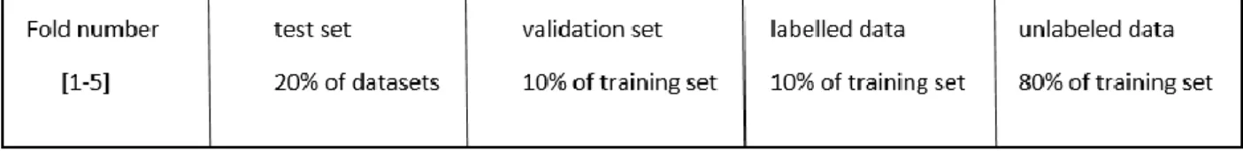
As can be seen simply applying a Support Vector Machine to the small set of labeled data, the accuracy is sensibly less than when the training set contains more labeled data. Following the protocol used in this thesis, the labeled data are 10% of training set, which is 80% of total data (the protocol will be illustrated in the next chapters).
20
However in real cases the only labeled data available are the data manually labeled, and for this reason they represent a relatively small quantity. The idea of semi-supervised learning is to use also unlabeled data, available from training set, to construct a better model of classification. Experimentally has been seen that this technique can provide better performance in data classification. In the next, some general assumptions about semi-supervised learning and its main drawbacks will be explained and then some base techniques (self-training, co-training and help training) and the algorithms used in the reference articles will be introduced.
2.3.1 Assumption for Semi-Supervised Learning
In many cases the semi-supervised learning techniques comport advantages respect to supervised learning. However there is an important prerequisite: the distribution of samples (labeled and unlabeled) have to be relevant for the classification problem. In other words, we could say that the knowledge of 𝑝(𝑥) that one gains through the unlabeled data has to carry information that is useful in the inference of 𝑝(𝑦|𝑥). If this is not the case, semi-supervised learning will not yield an improvement over supervised learning. It might even happen that the usage of the unlabeled data degrades the prediction accuracy by misguiding the inference [2].
Semi-supervised smoothness assumption: if two points 𝑥1 and 𝑥2 in a high density region are closed, then so should be the corresponding outputs 𝑦1 and 𝑦2.
This Assumption follow from the smoothness assumption which say that two points close each other in the space of features should have the same label. Intuitively this is important to make possible a generalization from a finite training set to a set of possibly infinitely many unseen test cases.
For example, if many points in the same region of features space have different labels, it’s difficult for a classifier (for example a SVM) to determine a boundary dividing the classes. Moreover when
21
this boundary can be found, it’s not very significant in test phase when test samples, for hypothesis, can be arbitrarily of one of the classes (because they are in a high density region).
Cluster Assumption: if points are in the same cluster, they are likely to be of the same class. This assumption is based on the idea of use unlabeled data to better define the clusters of classes. In this hypothesis the labeled data can be divided in clusters and unlabeled data can be used to find the boundary of each class more accurately.
The cluster assumption can be easily seen as a special case of the semi-supervised smoothness assumption, considering that clusters are frequently defined as being sets of points that can be connected by short curves which traverse only high-density regions.
The cluster assumption can be formulated as follow:
Low density separation: The decision boundary should lie in a low-density region.
Intuitively we can see that a decision boundary in a high density region would cut a cluster into two different classes. The presence of many objects of different classes in the same cluster would require the decision boundary to cut the cluster and then the boundary will not lie in a low density region.
Manifold assumption: this assumption is about dimension of samples. Sometimes dimensions describing samples are too much (high-dimensional), so it’s useful to reduce the number of dimensions and represent the problem in a different (low-dimensional) space (manifold). The manifold assumption can be summarized as follow:
22
2.3.2 Semi-supervised algorithms
Semi-supervised learning strategies can be divided in classes of algorithms, considering the used approach. For example four classes of algorithms can be defined, based on the following approaches [2]:
Generative models: under the name generative models we refer to architectures following the generative paradigm described above. However quite all SSL algorithms are involved in the estimation of P(x|y) and from that derives the class probability estimation, instead of calculate it directly. So are classified as Generative models only technics strongly oriented to the determination of 𝑃(𝑥).
Low-Density separation: this class contains algorithms which try to directly implement the low-density separation assumption by pushing the decision boundary away from the unlabeled points. The most common approach to achieving this goal is to use a maximum margin algorithm such a Support Vector Machine considering also unlabeled data (for example transductive SVM).
Graph-Based Method: During last years, graph-based methods has been a very active area of research in semi-supervised learning. The common denominator of these methods is that the data are represented by the nodes of a graph, the edges of which are labeled with the pairwise distances of the incident nodes (and a missing edge corresponds to infinite distance).
23
Change of Representation: these algorithms are not intrinsically semi-supervised, but instead perform a two-step learning.
1. Perform an unsupervised step on all data, labeled and unlabeled, but ignoring the available labels. This can for instance, be a change of representation, or the construction of a new metric or a new kernel.
2. Ignore the unlabeled data and perform supervised learning using the new distances, representation or kernel.
This can be seen as direct implementation of the semi-supervised smoothness assumption, since the representation is changed in such a way that small distances in high-density regions are conserved.
Considering the different approaches, a Semi-Supervised Learning algorithm can combine some of them, or use other techniques like clustering. In the following, some popular SSL algorithms and basic approach to the SSL problem will be introduced.
2.3.3 Self-training
Self-Training is based on the idea of classifying progressively unlabeled data, adding to the pool of labeled data the records which have, at each step, a high ‘confidence’ in classification [8] [10]. In Self training a classifier is trained on an initial small amount of labeled data and is used to classify unlabeled data. For each classified element, is define a confidence measure which represent the ‘validity’ of assigned label. For SVM the confidence measure is usually the probability estimation, or the absolute value of the distance from the boundary. Both this values can be obtained in output of libSVM tool.
24
The most confident elements obtained from this step are added to the labeled data with the relative label resulting from classification, then the classifier is re-trained on new labeled data. The process is iterated until unlabeled data are less than a threshold parameter.
Self-training is characterized by the fact that the learning process uses its own predictions to teach itself. For this reason, it’s also called self-teaching or bootstrapping (not to be confused with the statistical procedure with the same name). Self-training can be either inductive or transductive, depending on the nature of the predictor 𝑓.
This semi-supervised learning method [10] is very simple to implement and has been applied successfully to several natural language processing task. In [26] self-training is used for word sense disambiguation, e.g. deciding whether the word ‘plant’ means a living organism or a factory in a given context. It has been used also to identify subjective nouns [27] and classify dialogues as ‘emotional’ or ‘non-emotional’ with a procedure involving two classifiers [28]. Self-training has also been applied to parsing and machine translation. In [29] self-training is applied to object detection systems from images, and shows how the semi-supervised technique compares favorably with a state-of-the-art detector.
Self-training is a very simply SSL algorithm to implement; is a wrapper method and it can be used in many complex algorithms. A disadvantage is, for example, that early classification errors can
Self-training
Input: labelled data {(𝒙𝒊, 𝑦𝑖)}𝑖=1𝑙 , unlabeled data {𝒙𝒋}𝑗=𝑙+1𝑙+𝑢 1. Initially, let 𝐿 = {(𝒙𝑖, 𝑦𝑖)}𝑖=1𝑙 and 𝑈 = {𝒙𝒋}𝑗=𝑙+1𝑗=𝑙+𝑢 2. Repeat
3. Train 𝑓 from 𝐿 using supervised learning 4. Apply 𝑓 to the unlabeled data instances in 𝑈
25
‘propagate’ themselves and affect final accuracy, moreover there is a problem of convergence of the algorithm.
2.3.4 Co-training
Another popular algorithm for semi-supervised learning is co-training. This algorithm was originally proposed in [15]. In this technique two classifiers work together to perform label propagation. The classic approach of co-training is to train two classifiers separately based on two sufficient and redundant feature subsets (views), and then recover the most confident data for each other as the new labeled data. For this approach, there are strong assumptions on the feature sets.
Remark 2.3.1 Co-training Assumptions
Features can be divided into two subsets and each subset is sufficient to learn a good classifier
Two features subsets are conditionally independent given the class.
The first assumption on features independence is quite strong, since in a general dataset features has some kind of correlation between each other. In order to relax this assumption, variations of the algorithm have been proposed: a class of algorithms of co-learning, which doesn’t need a features separation for the two classifiers. Two learners, or an ensemble of learners, are trained separately on the full feature set of the labeled training data and then labels are predicted on the unlabeled data separately. In the case of an ensemble of learners a majority voting is used in order to determine the classification of unlabeled data.
Another variation of co-training is tri-training, proposed in [16]. In this algorithm three learners are used in the learning process. In detail, training data are generated by bootstrap sampling from initial data source. Then three hypotheses are trained based on these data. In the learning process, when two
26
learners agree with the classification of a new unlabeled sample, their prediction label will be marked on the unlabeled sample for the third learner. Three initial learners were updated during the tri-training process and the final hypothesis is determined by the majority voting.
Co-training model has practical applications in many real world cases. For example co-training model was applied for the named entity classification in the natural language process. Co-training with error-correcting output codes (ECOC) was applied for text classification. For visual detection, co-training has reduced the false positive rate significantly. It has also been successfully applied to email classification and statistical parsing [10].
2.3.5 Help training
Help-training is a semi-supervised algorithm proposed in [17]. The idea of this algorithm is to use a classifier based on a generative model to ‘help’ a classifier which uses discriminative approach. Let consider the main classifier 𝐶which is based on a discriminative approach and the classifier 𝐺 based on a generative model. The classifier 𝐺produces a probability density model. It tries to find the basic information of each class by modeling the data. In Help-Training, the classifier 𝐶is helped by 𝐺 to make decisions about which samples can be labeled and added to the training set. So, at each iteration, the classifier 𝐺is used to select the samples which have a high probability to belong to each class. These selected samples constitute the candidate samples for labeling process. The classifier 𝐶 classifies the pre-selected samples and those that are classified with highest scores are added to the training set. The process is repeated until all unlabeled data are labeled.
27
2.3.6 Adaptive bootstrap
Adaptive bootstrap is a supervised classification technique which train a group of different classifiers (usually decision tree) on different datasets constructed from the original dataset by bagging with replacement 𝑛 ≤ 𝑁 data, where 𝑁 is the dimension of the original dataset. Then, from this initial group of classifiers, a single learner it is derived combining together the classifiers.
This technique provides good results and so it’s quite diffused.
For the experiments of this work the MATLAB library adaboost is used, which follows the syntax:
for the training the function fitensamble is used:
Ensemble = fitensemble(X,Y,Method,NLearn,Learners, Name,Value)
Input:
X: data
Y: labels
Method: the method of classification: for classification with Ada Boost, this parameter is the string ‘AdaBoostM1’
NLearn: the number of ensemble learning cycles, i.e. the number of times the entire procedure will be repeated
Learners: the basic kind of learner, typically decision tree
Pairs (Name, Value): define other options, for example a cost matrix.
Output:
Ensemble: the classifier built form the ensemble of learners
28
[predict_label,scores] = predict(Ensemble,data)
Input:
Ensemble: the ensemble of classifier obtained from fitensamble
Data: unlabeled data Output:
Predict_labels: predictions of the labels for input data
Scores: a measure relative to probability estimation
2.4 Risks of Semi-Supervised Learning
Empirical and theoretical results have often testify favorably to the semi-supervised learning of generative classifiers. However, the literature has also brought to light a number of situations where semi-supervised learning fails to produce good generative classifiers.
For example, [18] reports experiments where unlabeled data degraded the performance of Naïve Bayes classifiers with Gaussian variables. The authors attribute such cases to deviations from modelling assumptions, such as outliers or “samples of unknown classes”, they even suggest that unlabeled samples should be used with care, and only when the labeled data alone produce a poor classifier. Another representative example is [30], where classifiers sometimes display performance degradation. The authors suggest several possible sources of difficulties: numerical problems in the learning algorithm, mismatches between the natural cluster in feature space and the actual labels, etc. In [19], labeled and unlabeled data are used to learn Bayesian network classifiers, from naïve Bayes classifiers to fully connected networks. The naïve Bayes classifiers display bad classification performance, and in fact the performance degrades as more unlabeled data are used (more complex networks also display performance degradation as unlabeled samples are added).
29
A last example is provided in [20]. In the described experiments outliers are added to a Gaussian model, producing a performance degradation of generative classifiers.
2.4.1 Methodological Considerations
Given a pool of labeled and unlabeled data, generative semi-supervised learning is an attractive strategy. However, one should always start by learning a supervised classifier with the labeled data. This “baseline” classifier can then be compared to other semi-supervised classifiers through cross-validation or similar techniques. Whenever modelling assumption seem inaccurate, unlabeled data can be used to test modelling assumptions. If time and resources are available, a model search should be conducted, attempting to reach a “correct” model (that is a model where unlabeled data will be truly beneficial).
An additional step consists in the comparison of the baseline classifier to non-generative methods. There are many semi-supervised non-generative classifiers, and there are also a significant number of methods that uses labeled and unlabeled data for different purposes (for example methods where the unlabeled data are used only to conduct dimensionality reduction). However we should warn that a few empirical results in the literature suggest the possibility of performance degradation in non-generative semi-supervised learning paradigms, such as transductive support vector machine.
2.4.2 Active Learning
A final methodological comment concerns active learning. This technique consists in labelling selected samples among the unlabeled data, instead of use the entire set of unlabeled data. This option should be seriously considered whenever possible. In some cases has been observed that the most profitable usage of unlabeled data is to use these data as a pool of samples from which some samples
30
can be carefully selected and labeled. In general, we should take the score of a labeled sample to be considerably higher than the score of an unlabeled sample.
31
Chapter 3
Proposed system
This thesis is based on the implementation and combination of four state-of-art techniques described in the relative articles of reference. Then the techniques are combined together through specific protocols and the experiments result are shown.
In this chapter, the used algorithms will be explained. So the algorithms and articles are presented by a theoretical point of view in this chapter, while in the next chapter, tests and experiments will be proposed.
3.1 Reference Articles
3.1.1 DCPE co-training for classification
In [7] a method for semi-supervised classification is proposed. The idea is to use diversity of class probability estimation (DCPE) of two different classifiers to add progressively to labeled data the unlabeled data with high DCPE. This algorithm is based on the idea of co-training, which uses two different classifiers to evaluate ‘better’ unlabeled data which can be added to labeled data with a label predicted with high confidence.
32
To implement this approach two different supervised algorithms have been used: a support vector machine with polynomial kernel, and an implementation of adaptive bootstrap provided by MATLAB. The pseudocode of the algorithm is the described in Algorithm 3.1:
This algorithm implements a scheme of co-training, based on the diversity of class probability estimation. In ensemble learning, diversity plays an important role in combining different learners. There exists many different approaches to use diversity in learning process. Some of the most diffused are:
Pseudocode describing the DCPE co-training algorithm 1: Input: b1 baselearningalgorithm1 b2 baselearningalgorithm2 L labeled data U unlabeled data 2: Allocate LA = L, LB = L
3: Use b1 to train on LA to get a classifier hA, uses b2 to train on LB to get a classifier hB
4: Create a pool U’ by randomly choosing u data from U 5: if size(U) ≥ u then
6: Use hA and hB separately to predict each data x in U’: hA(x), hB(x). Record class
probability estimation (cpe) for each data: cpeA(x), cpeB(x)
7: Update LA= LA+ la , la are chose from U’, which have same prediction labels
(hA(x)= hB(x)) and the highest class probability estimation differences between hB
and hA:
𝑥 = 𝑎𝑟𝑔max
𝑥 (𝑐𝑝𝑒𝐵(𝑥) − 𝑐𝑝𝑒𝐴(𝑥))
8: Update LB= LB+ lb , lb are chose from U’, which have same prediction labels
(hA(x)= hB(x)) and the highest class probability estimation differences between hA
and hB:
𝑥 = 𝑎𝑟𝑔max
𝑥 (𝑐𝑝𝑒𝐴(𝑥) − 𝑐𝑝𝑒𝐵(𝑥)) 9: Remove la, lb from U’
10: Randomly choosing new u data from U to replenish U’
11: Update hA by using b1 to train on LA, update hB by using b2 to train on LB
12: end if
33
Diversity based on features subsets: features are partitioned in two subsets and then a base classification algorithm is used in each subset to determine a measure of diversity. Then co-training algorithm is applied. This approach is also called two view co-training.
Random features splitting: instead of divide features in subsets, features are randomly selected. This approach was performed in email classification and provided results comparable or better than using the original and natural features partitions.
Use different base learning algorithms: this method establish two classifiers by applying two base learning algorithms on the whole features set. This kind of co-training is called single viewco-training, since diversity is calculated on the entire features set.
The implemented algorithm uses the third approach, which presents several advantages. It doesn’t require a feature selection and so it’s simpler and easy to implement. Moreover it doesn’t require the co-training assumptions to be satisfied; this means that is not necessary that each view of the dataset represents exhaustively the data structure, and the two view are not necessarily conditionally independent. This situation is very common in real cases, so this approach can be considered more robust for general practical applications.
algorithm description
The DCPE co-training algorithm is designed for binary classification, and can be converted to multiclass problem using a technique such as one-vs-all approach.
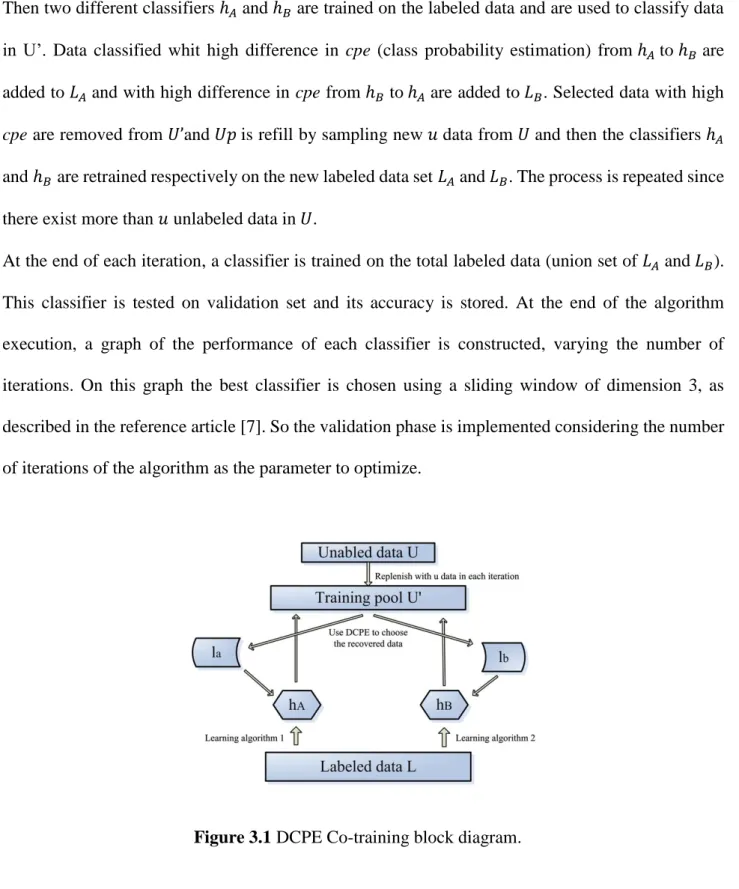
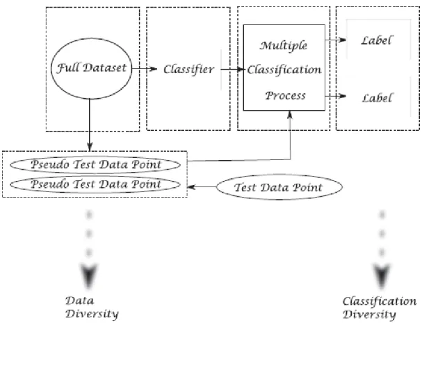
As shown in the block diagram of Figure 3.1, from unlabeled data 𝑈 are selected 𝑢 samples (in the experiments is used 𝑢 = 20) to form a pool of unlabeled data 𝑈’. It’s important to note that the selected data are removed from 𝑈 after selection.
Two labeled data sets are defined: 𝐿𝐴and 𝐿𝐵. Initially they are sets equal at the entire labeled data set 𝐿𝐴 = 𝐿𝐵 = 𝐿. In successive iterations 𝐿𝐴 will be updated with unlabeled data with high class probability estimation difference from ℎ𝐵classification to ℎ𝐴classification and vice versa for 𝐿𝐵.
34
Then two different classifiers ℎ𝐴 and ℎ𝐵 are trained on the labeled data and are used to classify data in U’. Data classified whit high difference in cpe (class probability estimation) from ℎ𝐴to ℎ𝐵 are added to 𝐿𝐴 and with high difference in cpe from ℎ𝐵 to ℎ𝐴 are added to 𝐿𝐵. Selected data with high
cpe are removed from 𝑈’and 𝑈𝑝 is refill by sampling new 𝑢 data from 𝑈 and then the classifiers ℎ𝐴 and ℎ𝐵 are retrained respectively on the new labeled data set 𝐿𝐴 and 𝐿𝐵. The process is repeated since there exist more than 𝑢 unlabeled data in 𝑈.
At the end of each iteration, a classifier is trained on the total labeled data (union set of 𝐿𝐴 and 𝐿𝐵). This classifier is tested on validation set and its accuracy is stored. At the end of the algorithm execution, a graph of the performance of each classifier is constructed, varying the number of iterations. On this graph the best classifier is chosen using a sliding window of dimension 3, as described in the reference article [7]. So the validation phase is implemented considering the number of iterations of the algorithm as the parameter to optimize.
analysis and conclusions
There exist many different basic machine learning algorithms that provide good performance in different kind of dataset and learning problems.
35
Most popular learning algorithms are such as Naive Bayes, neural networks, k-nearest neighbor, decision tree, and others. An advantage of using a co-training technique is that it can compare two different algorithms, and eventually can reveal performance differences in the usage of different pairs of algorithms for a specific dataset or learning problem. So it can be useful to investigate the ensemble learning approach with algorithms that approach data classification from different perspectives. Moreover, since diversity plays a critical role in ensemble learning methodology, the DCPE Co-training approach can also have an essential impact on the co-Co-training based algorithms.
The major advantages and positive aspects of DCPE Co-training approach can be summarized as follow:
DCPE co-training does not need the sufficient and redundant views (features subsets) of data set. The diversity of different learning algorithms is used to do label propagation. This can simplify the model and the implementation and, as said above, the single view co-training doesn’t require the satisfaction of the Co-training Assumptions (Remark 2.3.1).
A theoretical analysis can show how DCPE Co-training can achieve higher classification accuracy in co-training process. It can be proved that
Theorem 3.1.1: In the process of co-training, when the recovered data (with predicted labels) in i-th iteration have relatively smaller noise compared with labeled data, the learning
hypothesis can achieve lower error.
Competitive results among classical supervised learning methods and semi-supervised learning method (co-training, self-training and tri-training) are obtained on binary UCI data sets.
In the co-training process, the disagreement between two classifiers can be used for improving the final hypothesis. In DCPE Co-training method, is established the diversity between two classifiers, which shares similar property with disagreement-based co-training (a co-training approach proposed in [21]).
36
The key idea of this approach is to use the classification diversity from different learners for label propagation. It is a kind of ensemble learning approach based on the diversity of classifiers. The experimental results provided in [7] demonstrates that the proposed approach can achieve competitive results when it is compared with supervised learning methods and semi-supervised learning methods (co-training, self-training, and tri-training).
3.1.2 Using clustering analysis to improve semi-supervised
classification
In the reference article [9] is proposed an algorithm which uses semi-supervised clustering combined with a traditional supervised SVM to classify data.
Clustering is, in its simplest interpretation, an unsupervised learning technique. It is the classical unsupervised problem. It consists in the division of samples in distinct clusters, considering their distribution in the space of features. Typically these data are not labeled, for example data can be relative to webpages which need to be grouped by similar argument. In this case the possible arguments of pages are not known a priori, or the argument itself is not important for the learning purpose. Moreover there could be webpages not classified of a specific argument, and they must be grouped for similar topic of discussion.
The corresponding version of semi-supervised clustering is based on the fact that there are also labeled data in the dataset, and so these data must be considered in the clustering process. In the algorithm proposed in [9], the labeled and unlabeled data are firstly elaborate in a semi-supervised learning way through semi-supervised clustering, labels are assigned to unlabeled samples and unlabeled samples classified with high confidence are take into account. Then labeled data obtained
37
at the previous step are classified with a supervised SVM. Then the process is iterated updating the sets of labeled and unlabeled data.
In particular the ideas underling this approach of analysis are the following:
As unlabeled data may contain crucial information about the data space, clustering methods is used to reveal the underlying data space structure and to improve the training efficiency of the classifier.
Labeled data are used to guide the clustering process through semi-supervised clustering methods.
Newly labeled data are used not only to update the classifier (as in Self-training), but also to better guide the semi-supervised clustering methods.
The algorithm used to implement clustering is Semi-Supervised Fuzzy C-Mean (SSFCM), the semi-supervised version of Fuzzy C-Mean (FCM), a popular clustering algorithm.
semi-supervised fuzzy c-mean
As said before, SSFCM is the semi-supervised version of FCM. Fuzzy C-Means (FCM) is one of the most popular unsupervised clustering methods. In comparison to hard clustering, FCM provides an additional conceptual enhancement by allowing a data point to be assigned to different classes with various membership degrees. In this way, the patterns can be treated in a more reasonable way and the algorithm is capable of identifying eventual ‘‘outliers’’.
Let 𝑋 = {𝑥1, 𝑥2, … , 𝑥𝑛}, 𝑥𝑖𝜖ℝ𝑑 be a dataset of size 𝑛 and dimension 𝑑. Let’s consider a problem of clustering where 𝑐 is the number of classes and𝑉represents the set of prototypes associated with classes (prototypes are labeled samples chosen for each class).
The fuzzy c-mean solution of the problem consists in determining the partition matrix 𝑈 which minimize the following objective function:
38 min ℑ𝑚 = ∑ ∑ 𝑢𝑖𝑗𝑚 𝑛 𝑗=1 𝑐 𝑖=1 ∥ 𝑥𝑗− 𝑣𝑖 ∥2 (3.1) The superscript𝑚 is the degree of fuzziness associated with the partition matrix.𝑈 is a partition matrix whose element𝑢𝑖,𝑗 indicates the membership degree of the data point 𝑥𝑗to class 𝑖and satisfies two conditions:
0 ≤ 𝑢𝑖𝑗 ≤ 1 (3.2)
∑ 𝑢𝑖𝑗 = 1
𝑐 𝑖=1
Finally 𝑑𝑖𝑗 =∥ 𝑥𝑗− 𝑣𝑖 ∥2 expresses the distance between 𝑥𝑗 and 𝑣𝑖.
Semi-Supervised version of FCM clustering is based on the idea of use labeled data to improve the performance of clustering. Labeled data can be used for choosing the prototype 𝑣𝑖 and to provide additional information to the learning problem. Considering labeled data, the objective function to minimize assumes the following form:
min ℑ𝑚 = ∑ ∑ 𝑢𝑖𝑗𝑚 𝑛 𝑗=1 𝑐 𝑖=1 ∥ 𝑥𝑗− 𝑣𝑖 ∥2+ ∑ ∑ 𝑢′ 𝑖𝑗 𝑚 𝑛′ 𝑗=1 𝑐 𝑖=1 ∥ 𝑥′𝑗− 𝑣𝑖 ∥2 (3.3) Where the second term take into account the labeled data. Labeled data are 𝑋′ = {𝑥′1, 𝑥′2, … , 𝑥′𝑛} where 𝑥′𝑖𝜖ℝ𝑑. The partition matrix 𝑈’ defines the membership degree of each predicted value to each class 1, … , 𝑐 and must satisfy the following constraints
0 ≤ 𝑢𝑖𝑗 ≤ 1 (3.4) ∑𝑐 𝑢𝑖𝑗 = 1
𝑖=1
𝑢′𝑖𝑗 ≥ 𝑢′
𝑘𝑗 , ∀𝑘 ∈ {1,2, … , 𝑐} {𝑖}⁄ , 𝑗 = 1,2, … , 𝑛′ 𝑖𝑓 𝐿(𝑥′𝑗) = 𝑖
Respect to the supervised case, an additional constraint is added. This constraints means that, for labe1ed data, the membership degree of the effective class 𝑖 must be higher than the membership degree of each other class 𝑗 = 1 … 𝑐, 𝑗 ≠ 𝑖.
39
For data prototypes:
𝑣𝑖 = ∑ 𝑢𝑖𝑗 𝑚𝑥 𝑗+ ∑𝑛′𝑗=1𝑢′𝑖𝑗𝑚𝑥′𝑗 𝑛 𝑗=1 ∑ 𝑢𝑖𝑗𝑚+ ∑ 𝑢′ 𝑖𝑗 𝑚 𝑛′ 𝑗=1 𝑛 𝑗=1 (3.5)
For unlabeled data point 𝑥𝑗:
𝑢𝑖𝑗 = 1 ∑ (𝑑𝑑𝑖𝑗 𝑙𝑗) 2/(𝑚−1) 𝑐 𝑙=1 (3.6)
For labeled data point 𝑥′𝑗
𝑢′𝑖𝑗 = 1 ∑ (𝑑′𝑖𝑗 𝑑′𝑙𝑗) 2/(𝑚−1) 𝑐 𝑙=1 𝑖𝑓 𝐿(𝑥′𝑗) = 𝑖 (3.7) min {𝑢′𝑖𝑗, 1−𝑢′𝑖𝑗 ∑ (𝑑′𝑘𝑗 𝑑′𝑙𝑗) 2/(𝑚−1) 𝑐 𝑙=1,𝑙≠𝑖 }, ∀𝑘 ∈ {1,2, … , 𝑐}/{i}, if 𝐿(𝑥′𝑗) = 𝑖 proposed algorithm
The algorithm proposed in [9] is essentially a framework for semi-supervised classification where a semi-supervised clustering process (SSFCM) is integrated into Self-training.
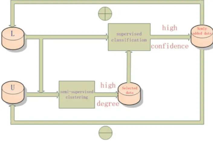
In the first phase, semi-supervised clustering uses both labeled and unlabeled data in the learning phase and assigns a label to unlabeled data, with the correspondent confidence degree (a measure of class probability estimation). Unlabeled data classified with higher level of confidence are selected for the supervised learning phase, while others values are left in the unlabeled set.
In the second phase, a supervised SVM is trained on labeled data and high-confidence classified unlabeled data with relative labels (provided by the first phase). The SVM is tested on the same
40
dataset used for learning, and data classified with high confidence are definitely added to labeled set, while other data are discarded and reinserted in the unlabeled set.
The two phase process is repeated until the unlabeled data are less than a parametric threshold. A diagram of the algorithm is represented in Figure 3.2. Then in the following the algorithm is presented in a more detailed way.
Figure 3.2 block diagram for Clustering and SVM algorithm.
Algorithm 3.2: Semi-supervised fuzzy c-means. SSFCM + SVM Pseudocode
Input: labeled dataset L(0) , unlabeled dataset U(0) Output: SVM classifier
Method:
1. Initialize the dataset L=L(0) and U=U(0), threshold values: ε1, ε2, N
2. Repeat until |U|≤N
– Estimate the membership degree using SSFCM for unlabeled data
– Select a dataset T1 where each sample xj has high certainty of belonging to one class.
– Train the SVM with L – Compute the output f(x) of the SVM for the selected dataset T1
– Select a dataset T2 where the output of each sample x by the SVM has high values. – Update the current labeled set 𝐿 ← 𝐿 ∪ 𝑇2
– Update the current unlabeled set 𝑈 ← 𝑈 − 𝑇2
– Reduce the value of ε1 if T2=∅
3. Label the remaining unlabeled data with the trained SVM, if U≠ ∅ 4. Retrain the SVM
41
In this implementation is important to note the thresholds 𝜀1 and 𝜀2. They represent the threshold for confidence respectively in the clustering semi-supervised classification and in the SVM supervised phase. When 𝑇2 is empty, the value of 𝜀1 is reduced of 0.05, as described in the reference article [9]. This guarantee the convergence of the algorithm (since there is a value of threshold 𝜀1 that allows to add enough element to labeled set) and the while loop will terminate.
3.1.3 A semi-supervised feature ranking method with ensemble
learning
This article [8] presents a method to determine a ranking of features, based on their importance in learning algorithm.
The proposed framework is based on semi-supervised learning, more precisely it uses a simple but efficient and easy to implement Self-training approach.
Feature selection consists in selecting a subset of relevant features, which achieves a better performance in accuracy for many learning problems with a large number of features.
Feature selection techniques provide three main benefits when constructing predictive models:
Improved model interpretability: in many cases there is a large number of features and many of them are irrelevant or almost irrelevant for the purpose of classification. However is not known which features are irrelevant and which not, so it may be useful a feature ranking algorithm
Shorter training times: training time is linear or exponential correlated to the number of features (it depends on the learning algorithm); so, reducing the number of features, the learning time can be considerably decreased.