Nonparametric density and survival function estimation
in the multiplicative censoring model
Elodie Brunel, F Comte, V Genon-Catalot
To cite this version:
Elodie Brunel, F Comte, V Genon-Catalot. Nonparametric density and survival function esti-mation in the multiplicative censoring model. Test, Spanish Society of Statistics and Operations Research/Springer, 2016, 25 (3), pp.570-590. <10.1007/s11749-016-0479-1>. <hal-01122847>
HAL Id: hal-01122847
https://hal.archives-ouvertes.fr/hal-01122847
Submitted on 4 Mar 2015
HAL is a multi-disciplinary open access archive for the deposit and dissemination of sci-entific research documents, whether they are pub-lished or not. The documents may come from teaching and research institutions in France or abroad, or from public or private research centers.
L’archive ouverte pluridisciplinaire HAL, est destin´ee au d´epˆot et `a la diffusion de documents scientifiques de niveau recherche, publi´es ou non, ´emanant des ´etablissements d’enseignement et de recherche fran¸cais ou ´etrangers, des laboratoires publics ou priv´es.
IN THE MULTIPLICATIVE CENSORING MODEL
E. BRUNEL, F. COMTE, AND V. GENON-CATALOT
Abstract. In this paper, we consider the multiplicative censoring model, given byYi=XiUi
where (Xi) are i.i.d. with unknown density f onR, (Ui) arei.i.d. with uniform distribution
U([0,1]) and (Ui) and (Xi) are independent sequences. Only the sample (Yi)1≤i≤n is observed.
Nonparametric estimators of both the densityf and the corresponding survival function ¯F are proposed and studied. First, classical kernels are used and the estimators are studied from several points of view: pointwise risk bounds for the quadratic risk are given, upper and lower bounds for the rates in this setting are provided. Then, an adaptive non asymptotic bandwidth selection procedure in a global setting is proved to realize the bias-variance compromise in an automatic way. When theXi’s are nonnegative, using kernels fitted forR+-supported functions,
we propose new estimators of the survival function which are proved to be adaptive. Simulation experiments allow us to check the good performances of the estimators and compare the two strategies.
Keywords. Adaptive procedure. Bandwidth selection. Kernel estimators. Multiplicative cen-soring model.
AMS 2000 subject classifications. 62G07 - 62N01
1. Introduction
In this paper, we consider the model
(1) Yi =XiUi, i= 1, . . . , n
under the assumptions: theUi,i= 1, . . . , n are independent and identically distributed (i.i.d.) with uniform distribution on [0,1]; the Xi, i = 1, . . . , n are real valued, i.i.d., with unknown densityf and cumulative distribution function (c.d.f.) F; the sequences (Ui)1≤i≤nand (Xi)1≤i≤n are independent. We intend to propose estimation methods for f and F (or ¯F = 1−F) when observing a sample (Yi)1≤i≤n only.
Model (1) has been widely investigated mostly when the random variablesXiare nonnegative. In this case, Model (1) is usually called themultiplicative censoring modeland was introduced in Vardi (1989), studied in more details in Vardi and Zhang (1992) and by Asgharianet al.(2012). As explained in Vardi (1989), the multicative censoring model unifies several important statis-tical problems (deconvolution of an exponential variable, estimation under decreasing density constraint or some estimation problems in renewal processes). However in the above quoted pa-pers, authors assume that observations are composed of two independent samples, one of direct observations X with size m, in addition to the above Y n-sample. The statistical procedures for estimating the c.d.f. F rely on the fact thatm tends to infinity and cannot be applied for
Date: March 4, 2015.
Universit´e Montpellier, I3M UMR CNRS 5149. email: [email protected].
Universit´e Paris Descartes, MAP5, UMR CNRS 8145. email: [email protected] . Universit´e Paris Descartes, MAP5, UMR CNRS 8145. email: [email protected].
m = 0. Let us mention that van Es et al. (2000) studied a survival analysis model involving both multiplicative censoring and length bias, in a parametric context.
The problem may be related to the moment problem: in Model (1), all moments of X can easily be estimated from the observationsY, so the question of distribution reconstruction from its moments as pointed out by Mnatsakanov (2006) can be addressed.
Another strategy is to take the logarithm of the squared model, as proposed in stochastic volatility models (see van Es et al. (2005), Comte and Genon-Catalot (2006)), and to apply deconvolution methods. In these papers, the Ui’s are supposed to be Gaussian. But then, the estimated function is distorted and, in case of real random variablesXi, information about their sign is lost, when proceeding so.
Series expansion methods have been proposed in Andersen and Hansen (2001): they consider the problem as an inverse problem and apply Singular Value Decomposition in different bases to provide estimators. They obtain rates comparable to ours though on different regularity spaces, however their procedure is not adaptive and depends on the choice of a cutoff which is only empirically studied. Later on, wavelet methods have been applied by Abbaszadeh et al.(2012,2013) to estimate the density and its derivatives, considering a generalLp-risk, and in presence of additional bias. Their estimators are adaptive and reach the same rates as ours up to logarithmic terms (when p= 2). They do not provide lower bound, and consider neither global estimation of the density (wavelets are compactly supported) nor survival function estimation. Note that Chesneau (2013) studies the multiplicative censoring model when the sequence (Xi)i∈N
is α-mixing and the Ui’s can be a product of independent uniform random variables. The dependence implies an important loss in the rate.
In this paper, we consider first the case where theXi’s are real-valued, and we investigate the pointwise nonparametric estimation on Rof bothf and the survival function ¯F(x) = 1−F(x).
All nonparametric methods (likelihood, projection, kernel, . . . ) rely on relationships between the density fY and survival function ¯FY = 1−FY of Yi and those ofXi, given by
(2) ∀y∈R, fY(y) = Z +∞ y f(x) x dx1y≥0+ Z y −∞ f(x) |x| dx1y<0,
(3) ∀y∈R, F¯Y(y) +yfY(y) = ¯F(y),
which imply the following key property. Lett:R→Rbe bounded, derivable, witht0 belonging
toL2(R), and assume that E|X|<+∞, then
(4) E(t(Y) +Y t0(Y)) =Et(X).
This relation allows us to propose adequate correction of the observation Y in order to get information about X, and yields simple kernel estimators of f and ¯F (see Formulae (7) and (5)). We first study their pointwise L2-risks properties. Under regularity assumptions, we can obtain rates of convergence for which lower bounds are provided. The study includes the classical case of nonnegative Xi’s, for which pointwise kernel estimation of the density and the survival function is new.
Then we study the global risk forf onRor for ¯F onR+ when the variables are nonnegative.
An adaptive choice of the bandwidths is proposed following the Goldenshluger and Lepski (2011) theory and proved to lead to automatic bias-variance tradeoff for the resulting adaptive density or survival function estimators.
Next, still considering nonnegative Xi’s, we use convolution power kernel estimators fitted to nonparametric estimation of functions onR+, proposed in Comte and Genon-Catalot (2012)
for standard density estimation. We introduce estimators of f,F¯ (now on R+), different from
require the choice of an integer parameter m, for which a data driven procedure is proposed. The resulting estimator is proved to be adaptive.
The paper is organized as follows. Standard kernel estimators are described and studied in Section 2, and convolution power kernel method is explained in Section 3. Section 4 presents a simulation study that allows us to compare the two strategies. Lastly, proofs are gathered in Section 5.
2. Kernel estimation on the real line
2.1. Definition of kernel estimators. Let K:R→Rbe a kerneli.e. an integrable function
with R
K(u)du= 1, which is also assumed to be square integrable. We set for h >0,Kh(u) = (1/h)K(u/h). Along the results hereafter, we possibly need additional conditions on K:
(A1) K is bounded.
(A2) K is an even function with limu→+∞K(u) = 0,K is derivable and K0 is integrable.
(A3) R[K0(u)]2du <+∞.
(A4) R|u|[K0(u)]2du <+∞.
(A5) R
[uK0(u)]2du <+∞. The estimator of ¯F(x) is defined by:
ˆ ¯ Fh(x) = 1 nh n X i=1 Z K u−x h 1IYi≥udu+YiK Yi−x h = Kh?Fˆ¯Y(x) + 1 n n X i=1 YiKh(Yi−x) (5)
wheres ? t(x) =R s(x−u)t(u)dudenotes the convolution product and
(6) Fˆ¯Y(x) = 1 n n X i=1 1IYi≥x.
ForK satisfying (A2), which implies(A1), we define the estimator off(x) by: ˆ fh(x) = 1 nh n X i=1 Yi hK 0 Yi−x h +K Yi−x h = 1 n n X i=1 YiKh0 (Yi−x) +Kh(Yi−x) . (7)
With simple computations, we can prove:
Proposition 2.1. Under (A2),
(i) Z ˆ fh(x)dx= 1, (ii) lim x→−∞ ˆ ¯ Fh(x) = 1, (iii) lim x→+∞ ˆ ¯ Fh(x) = 0, (iv) ( ˆF¯h)0(x) =−fˆh(x). 2.2. Pointwise risk. Consider the H¨older ball:
ΣI(β, R) ={f :I →R, f(`)exists for`=bβc,|f(`)(x)−f(`)(x0)| ≤R|x−x0|β−`,∀x, x0 ∈I}
wherebβcis the largest integer strictly smaller than β. Recall thatK is a kernel of order `if: Z
|u|`|K(u)|du <∞ and Z
ujK(u)du= 0 for j= 1, . . . , `.
Proposition 2.2. Assume that E(|X1|)<+∞.
Let x0 ∈R. Assume thatf belongs to ΣI(β, R)for I a neighborhood of x0. If the kernelK is of
order `+ 1 with`=bβc andR
|u|β+1|K(u)|du <+∞, then under (A1),
(8) E[( ˆF¯h(x0)−F¯(x0))2]≤C12h2(β+1)+ C2 nh + C3 n , (9) E[( ˆF¯h(0)−F¯(0))2]≤C12h2(β+1)+ C4 n , with C1 = R R |u|β+1|K(u)|du/(`+ 1)!, C 2 = 2E(|X1|)kKk2, C3 = 2kKk2 and C4 = 2kKk2 + R |u|K2(u)du.
If K is of order ` with ` = bβc and R |u|β|K(u)|du < +∞, then under (A2)-(A3), for all h∈(0,1), we have (10) E[( ˆfh(x0)−f(x0))2]≤C52h2β+ C6 nh3 with C5 =R R
|u|β|K(u)|du/`! andC
6 = 2 E(|X1|)kK0k2+kKk2∞
. Under (A2)-(A4), for x0= 0, we have
(11) E[( ˆfh(0)−f(0))2]≤C52h2β+
C60 nh2,
where C60 =kKk∞+R|u|[K0(u)]2du.
Under (A2)-(A3) and (A2), if E(1/|X|) =kfYk∞<+∞, kfk∞<+∞, andx0= 0, we have
(12) E[( ˆfh(0)−f(0))2]≤C25h2β+ C600 nh, where C600=kfk∞kKk2+kfYk∞ R u2[K0(u)]2du.
Forh of ordern−1/(2β+3), the estimator of ¯F(x0) has rateO(n−2(β+1)/(2β+3)), except in 0, where
choosing h = n1/[2(β+1)], gives the parametric rate. This is due to the fact that P(X > 0) = P(Y > 0) and thus ¯F(0) = ¯FY(0). For instance, n−1Pni=01IYi≥0 is an estimator of ¯F(0) with
parametric rate.
Forhof ordern−1/(2β+3), the estimator off(x
0) has rateO(n−2β/(2β+3)) whenx06= 0. The rate
is better atx0 = 0 and of orderO(n−2β/(2β+2)) orO(n−2β/(2β+1)), provided thatkfYk∞<+∞.
The next theorem states that the rates obtained for pointsx0 6= 0 are optimal-minimax.
Theorem 2.1. Assume thatx06= 0,x0∈I and let β >0.
There exists a constant c >0 such that
(13) liminf n→+∞n 2β/(2β+3) inf ˆ fn sup f∈ΣI(β,R) Ef h ( ˆfn(x0)−f(x0))2 i ≥c
where inffˆn denotes the infimum over all estimators of f based on (Yj)1≤j≤n.
Moreover, for β ≥1, there exists a constant c >0 such that
(14) liminf n→+∞n 2β/(2β+1) inf ˆ ¯ Fn sup ˆ ¯ F∈ΣI(β,R) Ef h ( ˆF¯n(x0)−F¯(x0))2 i ≥c
2.3. Global risk and bandwidth selection. We denote by kψk = (R
ψ2(x)dx)1/2 the L2
-norm and bykψk1 =R
|ψ(x)|dxtheL1-norm of a function ψ:R→R.
Letfh(x) = R
f(u)K((x−u)/h)/hdu=f ? Kh(x) and ¯Fh(x) = ¯F ? Kh(x). We can prove:
Proposition 2.3. Assume that E(X12)<+∞.
If f belongs toL2(R) and (A2)-(A3) hold, then
(15) E(kfˆh−fk2)≤ kf−fhk2+
kKk2
nh +
E(Y12)kK0k2
nh3 .
IfX is nonnegative,F¯ belongs toL2(R+)andK has compact support[−1,1], then, for allh≤1,
(16) E( Z R+ ( ˆF¯h(x)−F¯(x))2dx)≤ Z R+ ( ¯Fh(x)−F¯(x))2dx+ 2E(Y12)kKk2 nh + 2E(Y1+ 1)kKk21 n .
By considering Nikols’ki classes of functions (see Tsybakov (2009)) instead of H¨older classes, we may evaluate the bias order and deduce rates of convergence. As the regularity is not known, we rather propose a bandwidth selection strategy inspired from Goldenshluger and Lepski (2011), which yields a nonasymptotic risk bound result. To that aim, let
ˆ
fh,h0(x) =Kh0?fˆh(x), and ˆF¯h,h0 =Kh0 ?Fˆ¯h(x).
Note that, as the kernel is even, ˆfh,h0 = ˆfh0,h and ˆF¯h,h0 = ˆF¯h0,h. Let Hn be a finite set of
bandwidths. Then set A(h) = sup h0∈H n kfˆh0 −fˆh,h0k2−V(h0) +, B(h) = suph0∈H n kFˆ¯h0−Fˆ¯h,h0k2 R+−W(h 0 ) +, with (17) V(h) =κ1kKk21 k Kk2 nh + E(Y12)kK0k2 nh3 , W(h) =κ2kKk21 E(Y12)kKk2 nh ,
whereκ1 and κ2 are numerical constants.
For each estimator, the termA(h) (resp. B(h)) approximates the square bias term whileV(h) (resp. W(h)) is proportional to the variance term. Therefore, the data-driven bandwidths are defined by:
(18) ˆh= arg min
h∈Hn
(A(h) +V(h)), h?= arg min h∈Hn
(B(h) +W(h)).
The above definitions depend on the unknown moment E(Y12), which should be replaced by
n−1Pn
i=1Yi2. This substitution is possible both in theory and in practice. Note that kKk1 ≥
1 =R
K. The following holds:
Theorem 2.2. Assume thatf belongs toL2(R), E(X18)<+∞ and Hn is such that
(i) Card(Hn)≤n,
(ii) ∀a >0, ∃Σ(a)>0 such that P h∈Hnh
−2exp(−a/h)<Σ(a)<∞,
(iii) ∀h∈ Hn, 1/(nh3)≤1.
Then, under (A2)-(A3), there exists a numerical constantκ1 in V(h) defined by (17)such that
(19) E(kfˆˆh−fk2)≤c inf h∈Hn kKk21kf −fhk2+V(h) +c 0 n,
where c is a numerical constant and c0 depends onK and fY.
support [−1,1], then there exists a numerical constant κ2 in W(h) defined by (17) such that, (20) E( Z R+ ( ˆF¯h?(x)−F(x))¯ 2dx)≤c1 inf h∈Hn kKk21 Z R+ ( ¯Fh(x)−F¯(x))2dx+W(h) +c 0 1 n,
where c1 is a numerical constant and c01 depends onK and fY.
The proof delivers numerical values for the constantsκ1, κ2 which are too large. Finding the
minimal values is theoretically difficult. This is why it is standard to calibrate their value by preliminary simulations (see Section 4).
For instanceHn ={1/k, k= 1, . . . , n} or Hn ={2−k, k = 1, . . . ,log(n)/log 2}fulfill (i)-(ii). For (iii) the admissible values of kmust be restricted ton1/3 or log(n)/(3 log 2). Actually, (iii)
can be replaced by 1/(nh3)≤C for a constant C.
3. Convolution power kernel estimation on R+
Now, we assume that the Xi’s are nonnegative. The properties of the kernel estimators of f and the survival function ¯F of the previous section are still valid for x≥0 by setting f(x) = 0 for x < 0. However, for estimating functions on R+, it is often better to use appropriate
kernels so as to avoid the boundaries effects near 0. The convolution power kernels (Comte and Genon-Catalot (2012)) are well fitted to deal with this problem.
3.1. Definition of convolution power kernel estimators. For k a density on R+ with
expectation 1, we denote bykm the density of (E1+· · ·+Em)/mwithEi i.i.d. with density k,
i.e.
(21) km(u) =mk?m(mu), u≥0
where k?m =k ?· · ·? k, m times and? denotes the convolution product. Forh integrable, we denote by h∗(t) = R
eituh(u)du, t ∈ R its Fourier transform. The Fourier transform of km is given by
km∗(t) = (k∗( t m))
m, t∈
R.
For α1, . . . , αL real numbers such that PLj=1αj = 1,k(1), . . . , k(L) densities on R+ with
expec-tation 1, we define the convolution power kernel (CPK) by
(22) Km =
L X
j=1
αjkm(j).
The following assumptions are required on the densities k(j), forj= 1, . . . , L.
(B1)Foru≥0,k(j)(u)≥0, foru <0,k(j)(u) = 0,R+∞
0 k
(j)(u)du= 1,R+∞
0 (k
(j))2(u)du <+∞,
limu→+∞uk(j)(u) = 0, and
Z +∞
0
uk(j)(u)du= 1, ∃γ ≥4, such that Z +∞
0
|u−1|γk(j)(u)du <+∞
(B2) Form large enough, R+∞
0 k (j)
m (u)duu = 1 +O(m1).
(B3) There existsm0≥1 such that the functiont[(k(j))∗(t)]m0 belongs toL1(R)∩L2(R).
Now, we define forx >0, the estimator of ¯F(x) by: (23) F˜¯m(x) = 1 x Z +∞ 0 Km u x ˆ ¯ FY(u)du+ 1 nx n X i=1 YiKm Yi x . Under (B3),Km is derivable, so we can define, for estimating f(x) atx >0,
(24) f˜m(x) = 1 nx n X i=1 Km Yi x +Yi xK 0 m Yi x .
Proposition 3.1. Under (B1), we have limx→0+F˜¯m(x) = 1,limx→+∞F˜¯m(x) = 0.
Under (B1)-(B3), we have Z +∞ 0 ˜ fm(x)dx= 1 +O( 1 m).
3.2. Examples of kernels yielding explicit formulae. Examples of densities k leading to explicit formulae forkm are the following.
Example 1. Uniform kernels and splines. Let k(x) = (1/2)1I[0,2](x) the uniform density on [0,2]. Then Formula (9) in Killmann and von Collani (2001) (see also R´enyi (1970)) yields
km(x) = m (m−1)!2m bmx/2c X i=0 (−1)i m i (mx−2i)m−11I[0,2](x)
Here,kis not continuous on (0,+∞) and successive convolutions increase the regularity. Thus, the exponentmplays clearly the role of regularity parameter. Assumptions(B1)and(B3)hold.
Example 2. Gamma kernels. Forkthe Gamma density G(a, a),a >0,(B1)-(B3) hold and: km(u) =
(am)am Γ(am) u
am−1e−mau1 u>0.
Form >1/a,R0+∞u−1km(u)du= (am)/(am−1) = 1 +O(1/m).
Example 3. Inverse Gaussian kernels. The inverse Gaussian distributionIG(a, θ)a >0, θ >0, is defined as the distribution of the hitting time Ta = inf{t ≥ 0, θt+Bt = a} where (Bt) is a standard Brownian motion. The density of an IG(a, θ) is (a/√2πt3)eθae−(1/2)(θ2t+a2/t)
.For a = θ, the expectation is 1 and the variance is v = 1/a2. For k the inverse Gaussian density IG(a, a), (B1)-(B3) hold and km is the density of the lawIG(a
√ m, a√m): km(u) = a√m √ 2πu3e ma2(1−1 2( 1 u+u))1u>0, Z +∞ 0 u−1km(u)du= 1 + 1/(a2m).
3.3. Pointwise risk. To evaluate the order of the bias term, we need to define the notion of convolution power kernel of order`.
Definition 3.1. We say that Km =PLj=1αjk(mj) defines a convolution power kernel of order `
if, for j = 1, . . . , L, the density k(j) satisfies Assumptions (B1)-(B2), admits moments up to order ` and the coefficients αj, j = 1, . . . , L are such that PLj=1αj = 1 and for 1 ≤k ≤` and
allm (at least large enough)
Z +∞ 0 (u−1)kKm(u)du= L X j=1 αj Z +∞ 0 (u−1)kkm(j)(u)du= 0.
These relations allow to compute theαj’s as functions of the moments of thek(j)’s (see Comte and Genon-Catalot (2012)). Note that a single convolution power kernel withL= 1 is of order one.
Now, we can prove the following result.
Proposition 3.2. Let x0 > 0. Consider the estimator (23) built with a kernel (22) satisfying
(B1). Set (25) |α|1 := L X i=1 |αi|, vj = Z +∞ 0 (u−1)2k(j)(u)du, j = 1, . . . L.
If F¯ belongs toΣI(β, R)for I a neighborhood ofx0, the kernelKm is order `=bβcin the sense
of Definition 3.1 and forj= 1, . . . , L, R0+∞|u−1|βk(j)(u)du <+∞, then form,nlarge enough,
E[( ˜F¯m(x0)−F¯(x0))2]≤C1(β) x20β mβ + 4|α|1 L X j=1 |αj| p 2πvj √ m n + 2 |α|2 1 n
where C1(β) is a constant depending onR, β, the αj’s and the moments of the k(j)’s.
Assume moreover that (B2) and(B3) hold and f is bounded. Then,
E[( ˜fm(x0)−f(x0))2]≤C1(β) x20β mβ + C20kfk∞ √ m nx0 +C200( √ m)3 nx3 0 where C20 = 2P 1≤i,j≤L|αiαj|/ p 2π(vi+vj),C200 = 2 P 1≤i,j≤L|αiαj|/ p 2π(vi+vj)3)and C1(β)
is the same as above.
3.4. Global risk and adaptation. We prove a global result for ˜F¯m.
Proposition 3.3. Assume that(B1)holds andE(X1)<+∞. Then the integrated risk satisfies:
E Z +∞ 0 ˜ ¯ Fm(x)−F¯(x) 2 dx ≤ Z +∞ 0 EF˜¯m(x)−F¯(x) 2 dx+C2010 √ mE(Y1) n
where C20 is defined in Proposition 3.2.
Below, we do not search to link the bias term with the regularity property of the function ¯F. We rather focus on finding a data-driven value ofmwithout knowing the regularity of ¯F onR+.
From Propositions 3.2 and 3.3, √m plays the role of the bandwidth.
For two functionssandton (0,+∞), let us define, each time it exists on (0,+∞), the function u→st(u) =
Z +∞
0
s(u/v)t(v)dv/v.
If U1, U2 are nonnegative independent random variables with densities k1, k2 respectively, then
the product U1U2 has densityk1k2(u). Now, we define
(26) Mn={m=k2, log(n)≤k≤n/log(n)}
as the set of possible indexesmand considerKm=PLj=1αjk(mj), where the densitiesk(j) satisfy
(B1). Set (27) F˜¯m,m0(x) = 1 x Z +∞ 0 Km0Km u x ˆ ¯ FY(u)du+ 1 nx n X i=1 YiKm0Km Yi x .
AsKmKm0 =Km0Km, we have ˜F¯m,m0(x) = ˜F¯m0,m(x). Forκ a numerical constant and (28) C(K) = 2|α|31( L X i=1 |αi|/ √ 2πvi), we set (29) Z(m) =κC(K)E(Y1) √ m n , H(m) =msup0∈M n kF˜¯m0−F¯˜m,m0k2−Z(m0) +.
Note that, as |α|1 ≥1, the constant C20 of Proposition 3.3 satisfies
(30) C20 ≤2|α|1 L X j=1 |αj| p 2πvj ≤C(K).
The adaptive estimator is then ˜F¯m˜ with
(31) m˜ = arg min
m∈Mn
(H(m) +Z(m)).
As noted above, we should replace the unknown moment E(Y1) by its empirical counterpart.
This is no difficulty in the proofs. We can prove the following result:
Theorem 3.1. Assume thatF¯ belongs toL2((0,+∞)). Assume that (B1) holds andE(X14)<
+∞, then there exists a numerical constant κ such that
E Z +∞ 0 ˜ ¯ Fm˜(x)−F¯(x) 2 dx ≤C inf m∈Mn Z +∞ 0 EF¯m(x))−F¯(x) 2 dx+Z(m) +C 0 n ,
where C is a numerical constant and C0 a constant depending onE(X14) and on K.
Inverse Gaussian kernels (Example 3) are well fitted for practical implementation. Indeed if kis IG(1,1), then kmkm0 has the following explicit density
(32) kmkm0(u) = √ mm0 πu3/2 exp(m+m 0 ) ˜K0 m2+ (m0)2+m m0(u+ 1 u) 1/2!
where ˜K0 is the modified Bessel function of second kind with index 0 (available in R, library
Bessel), see Proposition 3.6 in Comte and Genon-Catalot (2012).
4. Simulations
In this section, we implement our estimators on simulated data. We have selected the following distributions:
Model 1: a Gaussian density,X ∼ N(2.5,0.75),
Model 2: a mixture of Gaussian densities,X∼0.5N(−2,1) + 0.5N(2,1), Model 3: a Gamma distribution,X ∼Γ(8,4),
Model 4: a rescaled Beta distribution,X = 5X0,X0 ∼β(3,3), Model 5: an Exponential distributionX ∼exp(2),
Model 1 Model 2 Model 3 Model 4 n= 200 500 200 500 200 500 200 500 Oracle Mean 0.022 0.014 0.007 0.005 0.022 0.015 0.013 0.006 (std) (0.014) (0.011) (0.003) (0.002) (0.017) (0.011) (0.008) (0.003) GL Mean 0.090 0.033 0.018 0.014 0.073 0.026 0.138 0.037 (std) (0.131) (0.05) (0.031) (0.015) (0.184) (0.018) (0.723) (0.065) Med. 0.045 0.009 0.014 0.009 0.036 0.021 0.020 0.011 CV Mean 0.403 0.269 0.215 0.109 0.297 0.126 0.509 0.314 (std) (0.705) (0.378) (0.448) (0.222) (0.518) (0.182) (1.031) (0.386) Med. 0.067 0.047 0.011 0.009 0.044 0.034 0.031 0.094 CV on X Mean 0.015 0.006 0.007 0.004 0.018 0.009 0.006 0.004 (std) (0.012) (0.004) (0.004) (0.002) (0.012) (0.007) (0.010) (0.002) Med. 0.013 0.005 0.007 0.004 0.015 0.008 0.009 0.004 Oracle on X Mean 0.004 0.002 0.003 0.002 0.004 0.002 0.003 0.002 (std) (0.003) (0.001) (0.002) (0.001) (0.003) (0.001) (0.002) (0.001)
Table 1. Table of risks for density estimators and oracles.
4.1. Density estimation. We consider the estimator given by (7) for Models 1 to 4, where K(x) is the standard Gaussian kernel. Bandwidths are selected between 0.1 and 1.5 in the set
Hn={0.1 + 0.05k, k= 0,1, . . . ,28}. For each sample, we compute:
- first, the oracle ˆfor= ˆfhor wherehor= arg minh∈Hnkfˆh−fk
2,
- second, the Goldenshluger and Lepski estimator ˆfˆh with ˆh given by (18) and κ1 = 1.2,
- third, the estimator ˆfhCV wherehCV is selected by a cross validation criterioni.e. minimizing
CV(h) = Z ˆ fh2(x)dx− 2 n n X i=1 [Yifˆh,0 [i](Yi) + ˆfh,[i](Yi)],
where ˆfh,[i] is the kernel estimator ˆfh computed on the sample without Yi (leave-one-out), - fourth, we compute the estimator of f based on the direct observations X1, . . . , Xn, ˆf
(X)
hCV,X
where ˆfh(X) is the standard kernel estimator off and hCV,X is the bandwidth selected by usual density cross-validation criterion (see e.g. Tsybakov (2009), Section 1.5),
- lastly, the oracle based on the direct observationsX1,· · · , Xn, also using the standard kernel estimator.
We investigate two sample sizesn= 200,500, and 50 repetitions. Table 1 gives the estimated
L2-risks of all estimators, together with medians and standard deviations except for the oracles.
As expected, the oracle on direct observations performs better than the one with censored data. The comparison between the GL method and the oracle on censored data shows that the GL method is stable and that the loss with respect to the oracle is stable. We stress that the GL method gives smaller risks than the CV method, much smaller for means, and still smaller for medians. Indeed, looking at both medians and standard deviations for the CV method, we can see that it is very unstable. This is the reason why we also experimented the CV method on the direct sample, but in this case, it behaves smartlier. We conclude that the estimator ˆfˆh
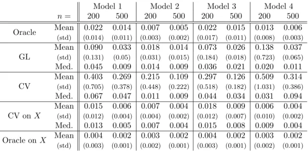
0 1 2 3 4 5 0.0 0.1 0.2 0.3 0.4 0.5 0.6 0.7 0 1 2 3 4 5 0.0 0.1 0.2 0.3 0.4 0.5 0.6 0.7 0 1 2 3 4 5 0.0 0.1 0.2 0.3 0.4 0.5 0.6 0.7 (a) (b) (c)
Figure 1. True density (solid black), oracle ˆfor (green) and estimators ˆfˆh (blue
dash-dotted), ˆfhCV (red dashed), ˆf
(X)
hCV,X (magenta long-dashed). n= 200 in (a)
and (b),n= 1000 in (c).
Model 3 Model 4 Model 5 Model 6 GL Mean 0.025 0.043 0.006 0.013 (std) (0.028) (0.038) (0.004) (0.012) Med. 0.015 0.027 0.005 0.012 Oracle GL Mean 0.010 0.014 0.004 0.009 (std) (0.009) (0.012) (0.009) (0.007) Med. 0.007 0.012 0.004 0.007 CPK Mean 0.021 0.034 0.005 0.017 (std) (0.015) (0.023) (0.005) (0.009) Med. 0.018 0.028 0.004 0.014 Oracle CPK Mean 0.013 0.021 0.004 0.011 (std) (0.011) (0.016) (0.003) (0.008) Med. 0.009 0.016 0.003 0.009
Table 2. Table of risks,n= 100 for survival function estimators and oracles.
estimator, the CV estimator on censored data and the CV estimator on direct data, for Model 3 with n = 200 (Figure 1 (a)-(b)), n = 1000 (Figure 1 (c)). When CV method works, it can be very competitive compared with GL method (see Figure 1 (a)), unfortunately, it sometimes completely fails as shown in Figure 1 (b). We can see on Figure 1 (c) that increasingnimproves the estimators.
4.2. Survival function estimation. For survival function estimation, we investigate for Mod-els 3 to 6 two couples of estimators:
- the Goldenshluger and Lepski-type kernel estimator ˆF¯h? given by (5) with h? given by (18)
withκ2 = 1, and the associated oracle ˆF¯h(GLor ), the bandwidths are selected among 30 equispaced
values between 0.01 and 0.9.
- the convolution power estimator ˜F¯m˜ given by (23) withκ= 0.5 and (31) with the inverse
Model 3 Model 4 Model 5 Model 6 Oracle GL Mean 0.004 0.005 0.001 0.003 (std) (0.003) (0.004) (0.001) (0.002) Med. 0.003 0.004 0.001 0.002 Oracle CPK Mean 0.005 0.008 0.001 0.004 (std) (0.003) (0.005) (0.001) (0.002) Med. 0.004 0.007 0.001 0.004
Table 3. Table of risks (n= 500)
Bessel), and its associated oracle ˜F¯mor. The values ofmare chosen among{5+3k, k= 0, . . . ,10}.
This is not exactly consistent with the theoretical constraint but computationally more tractable, with good results.
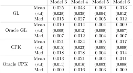
0.0 0.5 1.0 1.5 2.0 0.0 0.4 0.8 0.0 0.5 1.0 1.5 2.0 0.0 0.4 0.8
Figure 2. True survival function (solid black) and 10 estimators in dotted blue,
ˆ ¯
Fh? left (GL method), and ˜F¯m˜ right (CPK method), for Model 5 andn= 500.
Table 2 gives theL2-risks for sample sizen= 100 and 50 repetitions. Comparing L2-risks of
the GL and the CPK estimators, we find that the methods behave similarly and are stable over the four models. The difference between estimators and oracles is less important for survival function estimators (Table 2) than for density estimators (Table 1). For both methods, the loss between estimators and oracles is very small for Models 5, 6. The oracle of the GL method is much better than the estimator itself for Models 3, 4. This is less true for the CPK method.
Forn= 500 and 100 repetitions, theL2-risks of oracles are comparable (Table 3). In Figure
2, ten estimators of both methods for n = 500 are plotted together with the true function (bold), corresponding to Model 5. The GL method is on the left and the CPK on the right. Both methods yield convincing results and monotonic estimators. Although the CPK method is computationally slower, it provides better estimators, especially near zero (Figure 2).
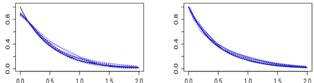
Figure 3 concerns Model 6, with still 10 estimators and n= 500. On top left and right, the GL and CPK estimators. As they are not always monotonic, we have used (bottom left and right) the monotonic transformation of estimators defined by (see Chernozhukovet al. (2009), R-package ’quantreg’):
¯
G7→G(y) = infˇ¯ {z; Z
One can prove that the risk of the monotonic version of any estimator on a bounded interval is smaller than the risk of the unmodified estimator. Finally, as the monotonic transformation leads to a step function, curves were smoothed using a method preserving monotonicity (R-function ’spline.fun’ of the method “monoH.FC” from Fritsch and Carlson (1980)). Clearly, the monotonic transformation improves the curves. The CPK method is better near zero, and the GL method seems better for large abscissa.
0.0 0.5 1.0 1.5 2.0 2.5 0.0 0.4 0.8 0.0 0.5 1.0 1.5 2.0 2.5 0.0 0.4 0.8 0.0 0.5 1.0 1.5 2.0 2.5 0.0 0.4 0.8 0.0 0.5 1.0 1.5 2.0 2.5 0.0 0.4 0.8
Figure 3. True survival function (solid black) and 10 estimators in dotted blue
for Model 6 and n = 500. Top left: ˆF¯h? (GL method). Top right ˜F¯m˜ (CPK
method). Bottom left: GL with monotonic transformation and smoothing. Bot-tom right: CPK with monotonic transformation and smoothing.
5. Proofs
We state a property used in proofs:
Lemma 5.1. Let ϕbelong to L2(R), E(Y2ϕ2(Y))≤E|X|kϕk2.
5.1. Proof of Equations (2)-(4) and of Lemma 5.1. Equality (2) is elementary. Fory≥0, ¯ FY(y) = Z +∞ y fY(z)dz = Z +∞ y Z +∞ z f(x) x dxdz= Z ( Z x y dz)f(x) x 1Iy≤xdx = Z +∞ y (x−y)f(x) x dx= Z +∞ y f(x)dx−y Z +∞ y f(x) x dx= ¯F(y)−yfY(y).
Fory≤0, FY(y) = Z y −∞ fY(z)dz = Z y −∞ dz Z z −∞ f(x) |x| dx= Z ( Z y x dz)f(x) |x| 1Ix≤ydx = Z y −∞ (y−x)f(x) |x| dx=yfY(y) +F(y)
Thus, ¯FY(y) = ¯F(y)−yfY(y),which is (3).
For (4), by (2), yfY(y) tends to 0 as both y tends to +∞ and −∞. By (3), EY2(t0(Y))2 is
finite. Integrating by parts yields Z R fY(y)(t(y) +yt0(y))dy = − Z R yt(y)(fY(y))0dy=−[ Z +∞ 0 yt(y)(−f(y) y )dy+ Z 0 −∞ yt(y)f(y) |y| dy] = Z +∞ −∞ t(y)f(y)dy.
Lemma 5.1 is immediate noting that EY2ϕ2(Y)≤EX2ϕ2(U X). 2
5.2. Proof of proposition 2.1. For (i), we useR
K0(u)du= 0 asK0is integrable andKis even, andR K(u)du= 1. For (ii) and (iii), we writeRKh(u−x)1IYi≥udu=
R
K(z)1Iz≤(Yi−x)/hdzfor the
first term and use that limu→+∞K(u) = 0 for the second term. Lastly (iv) is straightforward.
2
5.3. Proof of Proposition 2.2. First we study ˆfh. Noting that (yK(y−x h )) 0 y =K( y−x h ) + y hK( y−x h ), Equation (4) yieldsE( ˆfh(x)) =fh(x) =f ? Kh(x). Thus, for allx,
E[( ˆfh(x)−f(x))2] = (f(x)−fh(x))2+ Var h ˆ fh(x) i .
As K is of order ` = bβc, the assumption on f gives, at point x0,(f(x0)−fh(x0))2 ≤ C22h2β
withC2 =R
R
|u|β|K(u)|du/`! (see Tsybakov (2009) Proposition 2.1). Next, we have Var( ˆfh(x0)) ≤ 1 nh2E ( Y1 hK 0 Y1−x0 h +K Y1−x0 h 2) = 1 nh2 ( E " Y12 h2 K0 Y1−x0 h 2# +E K2 X1−x0 h ) (33)
where the last equality follows from Equation (4). Then
(34) E K2 X1−x0 h ≤min(hkfk∞kKk2,kKk2∞). By Lemma 5.1 , E " Y12 K0 Y1−x0 h 2# ≤ E(|X1|) Z (K0(u−x h )) 2du=h E(|X1|) Z (K0)2. Therefore, Var( ˆfh(x))≤(nh3)−1E(|X1|) R (K0)2+ (nh2)−1kKk2 ∞.This yields (10).
The special valuex0= 0 leads to other bounds. As,∀z∈R,|zfY(z)| ≤1, E " Y12 K0 Y1−x0 h 2# = Z
(x0+uh)2[K0(u)]2fY(x0+uh)hdu≤
Z
|x0+uh|[K0(u)]2hdu.
Therefore, for x0 = 0, we have
(35) E " Y12 K0 Y1 h 2# ≤h2 Z |u|[K0(u)]2du. Consequently, Var( ˆfh(0))≤ kKk∞+R |u|[K0(u)]2du nh2 := C60 nh2.
If nowfY is bounded and R
u2[K0(u)]2du <+∞, we get for x0 = 0,
(36) E " Y12 K0 Y1 h 2# ≤h3kfYk∞ Z u2[K0(u)]2du.
Thus if moreoverkfk∞<+∞, using (34),
Var( ˆfh(0))≤ kfk∞kKk2+kfYk∞ R u2[K0(u)]2du nh := C600 nh. This gives inequalities (11) and (12).
Now we study ˆF¯h to prove (8). First we have E( ˆF¯h(x)) = ¯F ? Kh(x) so that the bias term can be studied using Proposition 2.1 in Tsybakov (2009). Hence the bias order at x0. Next
Var( ˆF¯h(x)) ≤ 2 nh2 ( E Z K u−x h 1IY1≥udu 2 +E Y12K2 Y1−x h ) . (37) We have E Z K u−x h 1IY1≥udu 2 ≤ Z K u−x h du 2 =h2 Z |K(v)|dv 2 and E Y12K2 Y1−x h ≤hE|X1|kKk2.
Gathering terms gives (8).
Lastly, if x0 = 0, inequality (35) applies with K0 replaced by K and gives the result (9) and
thus ends the proof of Proposition 2.2. 2
5.4. Proof of Theorem 2.1. Proof of (13). To obtain lower bounds, we follow the reduction scheme described in Tsybakov (2009), chapter 2. We have to find two densities f0,n, f1,n such that
(i) fj,n∈ΣI(β, R),j = 0,1,
(ii) (f1,n(x0)−f0,n(x0))2 ≥cγn2 where γn2 is the desired rate,
(iii) χ2 =χ2(Pf1,n,Y, Pf0,n,Y)≤c/n, where Pf,Y is the law of Y when X has density f.
We only prove the result forx0 ∈(0,1) =I. Lethnbe small enough to have [x0−hn, x0+hn](
(0,1). We takef0,n(x) = 1I[0,1](x) and
f1,n(x) =f0,n(x) +cγnL(x
−x0
hn )
where L(v) = L(v)1I[−1,1](v), L ∈ ΣR(β, R), L(0) 6= 0 and R1 −1L(v)dv = 0. We set γn = n−β/(2β+3) and hn = n−1/(2β+3). We have R f1,n = R
f0,n = 1 and we can choose c such that f1,n(x)≥0,∀x∈[0,1], so thatf1,n and f0,n are [0,1]-supported densities.
(i) The functions fj,n,j= 0,1 are in ΣI(β, R) withI = (0,1) as γn/hβn= 1. (ii) (f1,n−f0,n)2(x0) =c2γn2L2(0) is of ordern−2β/(2β+3) =γn2, the expected rate.
(iii) Then we must prove thatχ2= Z 1 0 (g1−g0)2(x) g0(x) dx≤c/nwheregi(x) = R1 x(fi,n(u)/u)du, fori= 0,1. We have χ2 =c2γn2 Z 1 0 Rx 1 L(u−hnx0) u 1I[x0−hn,x0+hn]du 2 |log(x)| dx:=c 2γ2 n(I1+I2), with I1 = Z x0−hn 0 Rx0+hn x0−hn L(u−hnx0) u du 2 |log(x)| dx, I2= Z x0+hn x0−hn Rx0+hn x L(u−hnx0) u du 2 |log(x)| dx.
Using thatR−11L(v)dv = 0, we write
I1 = Z x0−hn 0 R1 −1 L(v) x0+vhnhndv 2 |log(x)| dx=h 2 n Z x0−hn 0 R1 −1 L(v) x0 1 1+vhn/x0 −1 dv 2 |log(x)| dx
and thus we get I1 ≤ h4 x2 0|log(x0)| Z x0−h 0 Z 1 −1 L(v) v/x0 1 +vh/x0 dv 2 dx ≤ h 4 x20(x0−h)2|log(x0)| Z x0−h 0 Z 1 −1 |L(v)|dv 2 dx= R1 −1|L(v)|dv 2 x20(x0−h)|log(x0)| h4. Next I2 =h2 Z x0+h x0−h 1 |log(x)| Z 1 (x−x0)/h L(v) x0+vh dv !2 dx≤ 2R1 −1|L(v)|dv 2 (x0−h)2|log(x0+h)| h3.
Thereforeχ2 ≤c(x0)γn2h3 =c(x0)/n which is the desired result. 2
Proof of (14). We seek a rate τn2 = n−2β/(2β+1). We build S0,n(x) = (1−x) for x ∈[0,1], the survival function associated tof0,n and
S1,n(x) =S0,n(x) +cτnL x−x0 hn forx∈[0,1],
with L0 =−L,L(x) = Rx1L(v)dv and L as above andL(0)6= 0. We take here τn =n−β/(2β+1) and hn =n−1/(2β+1). Note that S1,n is the survival function associated to ˜f1,n(x) =f0,n(x) + c(τn/hn)L((x−x0)/hn). Indeed τn/hn = n−(β−1)/(2β+1) is O(1) for β ≥ 1 so that c can be chosen small enough to have ˜f1,n≥0.
(i) The functions S0,n and S1,n are survival functions belonging to ΣI(β, R) with I = (0,1) as τn/hβn= 1.
(ii) (S0,n(x0)−S1,n(x0))2 =c2τn2L2(0).
(iii) For the χ2 distance between the observations laws, it follows the same lines as previously
and yields an order (τn2/h2n)×h3n, i.e. τn2hn=n−2β/(2β+1)×n−1/(2β+1)=n−1.
5.5. Proof of Proposition 2.3. The integrated mean-square risk is decomposed as the inte-grate of the squared bias plus the inteinte-grate of the variance. We inteinte-grate equation (33) and easily obtain bound (15).
Now we turn to (16). We start from (37) and get Z R+ Var( ˆF¯h(x)dx≤ 2 n Z R+ E Z (Kh(u−x) 1IY1≥udu 2 + 2 nhkKk 2 EY12 . Now we write Z R+ E Z (Kh(u−x) 1IY1≥udu 2 dx=E ( Z R+ Z (Kh(u−x) 1IY1≥u1Iu≥−1du 2 dx )
by interchanging expectation and integral and using that as K has support [−1,1], u ∈ [x−
h, x+h]⊂[−1,+∞) forx≥0 andh≤1. Therefore Z R+ E Z (Kh(u−x) 1IY1≥udu 2 dx=EkKh? gY1k 2
where gY1(u) = 1IY1≥u1Iu≥−1. Applying the Young Inequality (55) for p = 1, r =q = 2, yields
kKh? gY1k 2 ≤ kK hk21kgY1k 2=kKk2 1(Y1+ 1). This implies Z R+ Var( ˆF¯h(x)dx≤ 2 nkKk 2 1E(Y1+ 1) + 2 nhkKk 2 EY12 , and thus Inequality (16). 2
5.6. Proof of Theorem 2.2. We start by proving (19). By using the definitions ofA(h),V(h) and ˆh, we note that
∀h, h0 ∈ Hn, kfˆh,h0−fh0k2≤A(h) +V(h0),
and
∀h∈ Hn, A(ˆh) +V(ˆh)≤A(h) +V(h). Therefore, for allh∈ Hn,
kfˆˆh−fk2 ≤3kfˆˆh−fˆh,ˆhk2+ 3kfˆh,ˆh−fˆhk2+ 3kfˆh−fk2
≤3(A(h) +V(ˆh)) + 3(A(ˆh) +V(h)) + 3kfˆh−fk2
≤6A(h) + 6V(h) + 3kfˆh−fk2.
The termE(kfˆh−fk2) is ruled by Inequality (15) and we only need to studyE(A(h)). Recall that
ˆ
fh,h0 =Kh0 ∗fˆh, and denote fh(x) =E[ ˆfh(x)], fh,h0(x) =E[ ˆfh,h0(x)]. We split ˆfh := ˆf(1)
h + ˆf (2) h , fh :=f (1) h +f (2) h with ˆ fh(1)(x) = 1 nh n X i=1 [YiKh0(Yi−x) +Kh(Yi−x)]1I|Yi|≤cn, f (1) h (x) =E[ ˆf (1) h (x)],
and analogously for ˆfh,h0 and fh,h0. Then using the definition of A(h) we get A(h)≤5 sup h0∈H n n kfˆh(1)0 −f (1) h0 k2−V(h0)/10 o ++ 5 suph0∈H n n kfˆh,h(1)0 −f (1) h,h0k2−V(h0)/10 o + + 5 sup h0∈H n kfˆh(2)0 −f (2) h0 k2+ 5 sup h0∈H n kfˆh,h(2)0 −f (2) h,h0k2+ 5 sup h0∈H n kfh0−fh,h0k2 := 5(T1+T2+T3+T4+T5).
Using (55) with p= 1, q=r= 2, and kKh0k1 =kKk1, we obtain
T5 =kfh0−fh,h0k2=kKh0?(f−Kh? f)k2 ≤(kKk1)2kf−Kh? fk2. ForT1, we write T1= sup h0∈H n n kfˆh(1)0 −f (1) h0 k2−V(h0)/10 o +≤ X h∈Hn n kfˆh(1)−fh(1)k2−V(h)/10 o +,
and note that
(38) kfˆh(1)−fh(1)k2= sup
t∈L2(R),ktk=1
hfˆh(1)−fh(1), ti2= sup
t∈B(1)
hfˆh(1)−fh(1), ti2,
whereB(1) denotes a countable dense subset of{t∈L2(R),ktk= 1}.
Now we introduce the centered empirical process νn,h(ψt) =hfˆh(1)−fh(1), ti= 1 n n X i=1 [ψt(Yi)−E(ψt(Yi))], ψt(y) := Z y h2K 0 y−x h + 1 hK y−x h 1I|y|≤cnt(x)dx = yKh0 ? t(y) +Kh? t(y) 1I|y|≤cn. Therefore, E[T1]≤ X h∈Hn E "( sup t∈B(1) νn,h2 (ψt)−V(h)/10 ) + # .
We bound the above expectation using the Talagrand inequality (see Appendix). To apply it, we computeH, M and v. Clearly, H2 =V(h)/κ1 suits. Next, we get
sup t∈B(1) sup u∈R |ψt(u)| ≤ √ 2 h supu∈R Z c2 n h2(K 0)2 u−x h +K2 u−x h dx 1/2 ≤ √ 2 h c2n h kK 0k2+hkKk2 1/2 ≤C(K) cn h3/2 :=M.
Lastly, we search for v.
sup t∈B(1) Var (ψt(Y1))≤ sup t∈B(1) E ψ2t(Y1) . Remark that ψ2t(y) = n
y2(Kh0 ? t)2(y) +y(Kh? t)2(y) 0o 1I|y|≤cn. Thus by Equation (4), E(ψt2(Y1))≤EY12(K 0 h? t)2(Y1) +E(Kh? t)2(X1) :=S1+S2.
Next, by Lemma 5.1, Young’s Inequality (55) and asktk= 1, we get S1≤E(|X1|)kKh0 ? tk2≤E(|X1|)kKh0k21ktk2=E(|X1|)
kK0k2
1
h2 .
For S2, we write, applying twice the Young Inequality for r = +∞, p = q = 2 and p = 1,
q=r= 2 S2 = E[(Kh? t)2(X1)] = Z (Kh? t)2(x)f(x)dx≤ kKh? tk∞kKh? tkkfk ≤ kKhkktk kKk1ktk kfk= kKkk√Kk1 h kfk. Thus we getv=c(K, f)/h2wherec(K, f) =kK0k2
1E(|X1|) +kKk1kKkkfk. Then, forκ1/10 = 3 (= 1/2), we get E "( sup t∈B(1) νn,h2 (ψt)−V(h)/10 ) + # ≤ C1 n 1 h2exp (−C2/h) + c2 n nh3exp −C3 √ n cn . By the definition of Hn, we have 1/(nh3) ≤ 1, Ph∈Hnh
−2exp(−C
2/h) < Σ(C2) < ∞, and
Card(Hn)≤n. So, choosing
cn=C3
√
n/(4 log(n)),
we obtain E[T1] ≤c/n. The term T2 is studied analogously, with additional factorskKk21 due
to an additional application of Young’s Inequality.
For the terms T3, T4, rough bounds are used together with the definition ofHn, in particular 1/(nh3)≤1 to getT3≤C(K)nE(|Y1|2+p/cpn) for allp >0, whereC(K) is a constant depending on the kernel. Thus, with the definition of cn we obtain an order 1/n by choosing p = 6 with constraint E(|Y1|8)<+∞. Hence we get (19).
Now we turn to the proof of (20). The study follows the same line as previously, so we mainly give a sketch of proof. Here we can split in three parts ˆF¯h = ˆF¯h(1)+ ˆF¯h(2)+ ˆF¯h(3) with
ˆ ¯ Fh(1)(x) = 1 nh n X i=1 Yi1IYi<cnK Yi−x h , Fˆ¯h(2)(x) = 1 nh n X i=1 Yi1IYi≥cnK Yi−x h , ˆ ¯ Fh(3)(x) = Z Kh(u−x) ˆF¯Y(u)du, with ¯Fh(i) =E[ ˆF¯h(i)] fori= 1,2,3, and analogously for ˆF¯
(i)
h,h0,i= 1,2,3.
The first two terms are studied as previouslyT1, T2, T3, T4. There is also a term analogous to
T5. LetGY(u) = ( ˆF¯Y(u)−F¯Y(u))1I−1≤u. The additional new terms are
T6 :=E sup h0∈H n Z +∞ 0 [ ˆF¯h(3)0 (x)−F¯ (3) h0 (x)]2dx =E sup h0∈H n Z R+ [Kh0? GY(x)]2dx
and its twin in h, h0. Thus using Inequality (55) as previously, we get T6 ≤ E sup h0∈H n kKh0k21kGYk2 ≤ kKk21E Z ( ˆF¯Y(u)−F¯Y(u))21I−1≤udu = kKk 2 1 n Z
Var(1IY1≥u)1Iu≥−1)du≤
kKk2
1E(Y1+ 1)
n .
5.7. Proof of Proposition 3.1. For sake of simplicity, we assume that L = 1 and k(1) = k. By (B1), 1 x Z +∞ 0 km( u x)1IYi≥udu= Z Yi/x 0 km(v)dv≤ Z +∞ 0 km(v)dv= 1, so that ˜F¯m is well defined. Moreover, it is obvious from the formula above that
lim x→+∞ 1 x Z +∞ 0 km( u x) ˆF¯Y(u)du= 0, xlim→0+ 1 x Z +∞ 0 km( u x) ˆF¯Y(u)du= 1.
From Young’s Inequality (see (55) withr= +∞,p=q = 2) and(B1),kk ? kk∞≤ kkk2 so that
for all m≥2,kkmk∞<∞. Consequently,
lim x→+∞ 1 xkm( Yi x) = 0.
As uk(u) →0 when u →+∞, by induction we easily prove that ukm(u) → 0 when u → +∞. Therefore, lim x→0 1 xkm( Yi x) = 0.
In summary, we proved that, under (B1), limx→+∞F˜¯m(x) = 0 and limx→0+F˜¯m(x) = 1.
Without loss of generality, we assume that(B3) holds for m0 = 1 and write that
k(x) = 1 2π Z R e−itxk∗(t)dt, k0(x) = −i 2π Z R e−itxtk∗(t)dt.
This implies that k and k0 are continuous, tend to zero at +∞, and k(0) = k0(0) = 0. As km(y) =
Ry
0 k(y−z)km−1(z)dz for m > 1, we have km(0) = 0, limy→+∞km(y) = 0 and km is
continuously derivable, with
(39) (k0m)∗(t) =−itkm∗(t). Using(B2) and R+∞ 0 k 0 m(v)dv = [km(v)]+0∞= 0 yields Z +∞ 0 ˜ fm(x)dx= Z +∞ 0 km(v) dv v + Z +∞ 0 k0m(v)dv = 1 +O(1 m). 5.8. Proof of Proposition 3.2.
Lemma 5.2. Letk, k(1), k(2) satisfying(B1), then forv, v1,v2their variances(i.e. v=
R+∞ 0 (u− 1)2k(u)du), we have (40) kkmk2 = Z +∞ 0 km2(u)du=√m(1/2√πv(1 +o(1)), kkmk∞≤ √ m(1/ √ 2πv(1 +o(1)), (41) hk(1)m , km(2)i= Z +∞ 0
k(1)m (u)k(2)m (u)du=√m(1/p2π(v1+v2)(1 +o(1)).
Let k, k(1), k(2) satisfying(B1) and (B3), then
(42) kkm0 k2= 1 4√π m v 3/2 (1 +o(1)), h(k(1)m )0,(k(2)m )0i= √1 2π m v1+v2 3/2 (1 +o(1)).
Proof of Lemma 5.2. Equalities (40) and (41) are proved in Lemma A.1. of Comte and Genon-Catalot (2012).
Thus we turn to (42). Under(B1) and (B3) withm0= 1, as (km0 )∗(t) =−itkm∗(t),
kkm0 k2 = Z +∞ 0 (km0 (y))2dy= 1 2π Z R t2|km∗(t)|2dt= ( √ m)3 2π Z R s2|k∗(√s m)| 2mds.
Under the assumptionR t2|k∗(t)|2dt <+∞(see(B3)), we can mimick the proof of Lemma A.1.
(Comte and Genon-Catalot (2012)) to obtain: 1 (√m)3 Z R t2|km∗(t)2dt→ Z s2e−vs2ds= √ π 2v3/2.
And for the case of two densities,
h(k(1)m )0,(k(2)m )0i= Z +∞ 0 (k(1)m )0(y)(km(2))0(y)dy∼ ( √ m)3 2π Z R s2e−(v1+v2)s2/2ds. Hence (42). 2
Now we turn to the proof of Proposition 3.2. For the bias order, we have
E( ˜F¯m(x)) = 1 x Z +∞ 0 Km( u x) ¯FY(u)du+ 1 xE(Y1Km( Y1 x )) = 1 x Z +∞ 0 Km( u x) ¯FY(u) +ufY(u) du= 1 x Z +∞ 0 Km( u x) ¯F(u)du = Z +∞ 0 Km(v) ¯F(vx)dv.
The order of this term on ΣI(β, C), is given in Proposition 3.2 in Comte and Genon-Catalot (2012). Now, we bound the variance term.
Var( ˜F¯m(x)) = 1 nx2Var Z +∞ 0 Km( u x)1IY1≥udu+Y1Km( Y1 x ) ≤ 2 nx2 E[( Z +∞ 0 Km( u x)1IY1≥udu) 2] + E[Y12Km2( Y1 x )] :=T1(x) +T2(x) (43) T1(x)≤ 2 nx2 Z +∞ 0 |Km( u x)|du 2 ≤ 2 nx2 L X j=1 |αj| Z +∞ 0 k(mj)(v)xdv 2 = 2 n|α| 2 1, T2(x) = 2 nx2 Z Z ((uv)2Km2(uv
x )1I[0,1](u)f(v)1IR+(v)dudv= 2 nx2 Z +∞ 0 v2f(v) Z 1 0 u2Km2(uv x )du dv = 2 nx2 Z +∞ 0 f(v) v x 3 Z v/x 0 z2Km2(z)dz ! dv.
Thus using Lemma 5.2 namely R0+∞zk(mj)(z)dz= 1 and kkm(j)k∞≤2 √ m/p 2πvj), we get T2(x) ≤ 2 n Z +∞ 0 f(v) Z v/x 0 zKm2(z)dz ! dv≤ 2 n Z +∞ 0 zKm2(z)dz ≤ 2 nkKmk∞ Z +∞ 0 z|Km(z)|dz ≤ 2 n L X j=1 2|αj| √ m p 2πvj L X j=1 |αj| Z zkm(j)(z)dz ≤ 4|α|1 √ m n L X j=1 |αj| p 2πvj . Consequently we have Var( ˜F¯m(x))≤ |α|1 2 n |α|1+ 2 √ m L X j=1 |αj| p 2πvj .
Next, we study the estimator off. As (∂/∂y)(yKm(yx)) =Km(xy) + (y/x)Km0 (yx), we have
Ef˜m(x) = 1 xEKm( X1 x ) = Z +∞ 0 Km(v)f(xv)dv.
As for the bias term of ˜F¯m(x), the study of the bias term of ˜fm(x) is a direct application of Proposition 3.2 of Comte and Genon-Catalot (2012). For the variance term, we use that
Var ˜fm(x) ≤ 1 nx2E Km( Y1 x ) + Y1 x K 0 m( Y1 x ) 2 = 1 nx2 " EKm2( X1 x ) +E Y1 xK 0 m( Y1 x ) 2# We have EKm2( X1 x ) =x Z +∞ 0 Km2(v)f(xv)dv ≤xkfk∞kKmk2 where, by Lemma 5.2, theL2-norm of Km satisfies, using (30),
(44) kKmk2 ≤ √ m X 1≤i,j≤L 2|αiαj| p 2π(vi+vj) =C20√m≤C(K)√m.
For the other term, we have
E Y1 xK 0 m( Yi x) 2 = Z v≥0,0≤u≤1 (uv)2 x2 (K 0 m( uv x )) 2f(v)dudv = x Z +∞ 0 f(v) v dv Z v x 0 t2(Km0 (t))2dt ! ≤ 1 xE(X1) Z +∞ 0 (Km0 (t))2dt.
Now, we use (42) of Lemma 5.2
kKm0 k2 ≤ m 3/2 √ 2π X 1≤i,j≤L 2|αiαj| (vi+vj)3/2 . The result follows. This ends the proof of Proposition 3.2. 2
5.9. Proof of Proposition 3.3. Inequality (43) for Var( ˜F¯m(x)) must be integrated overR+.
The second term is the easiest: (45) Z +∞ 0 T2(x)dx≤ 2 nE(Y 2 1 Z +∞ 0 Km2(Y1 x ) dx x2) = 2 n E(Y1)kKmk 2.
For the term T1(x), we apply the generalized Minkowski inequality (see (54) in appendix):
Z +∞ 0 T1(x)dx ≤ 2 nE Z 1Ix≥0 dx x2 Z Km( u x)1IY1≥u1Iu≥0du 2 ≤ 2 nE " Z 1IY1≥u1Iu≥0du Z Km2(u x)1Ix≥0 dx x2 1/2#2 ≤ 2 nE " Z 1IY1≥u≥0 1 √ udu Z Km2(v)1Iv≥0dv 1/2#2 = 2 nE(2 p Y1)2) Z +∞ 0 Km2(v)dv = 8 nEY1kKmk 2. (46) Finally, Z +∞ 0 Var( ˜F¯m(x))dx ≤ 10 nEY1kKmk 2
which is the announced result using (44). 2
5.10. Proof of Theorem 3.1.
5.10.1. Some preliminary Lemmas. Let us set, form, m0 >0,
(47) BmF¯(x) =EF˜¯m(x)−F(x),¯ Bm,m0F¯(x) =EF˜¯m,m0(x)−F¯(x).
Similarly to Lemma A.3 of Comte and Genon-Catalot (2012), the following relation between bias terms holds.
Lemma 5.3. We have BmF¯(x) = R+∞
0 Km(u) ¯F(xu)du−F¯(x) and
Bm,m0F¯(x) =Bm0F¯(x) +
Z +∞
0
Km0(u)BmF¯(xu)du.
We also state a result with useful bounds concerning the convolution power kernels.
Lemma 5.4. Recall notations (25). Under assumptions (B1)-(B2), we have
(o) ||KmKm0||∞≤ |α|1PLj=1√|αj| 2πvj √ m∧m0(1 +o(1)). (i) kKmKm0k2 ≤C(K) √ m∧m0 where C(K) is defined by (28). (ii) R0+∞(|Km(z)|/ √ z)dz≤3|α|1. (iii) R+∞ 0 (|KmKm0(z)|/ √ z)dz ≤3|α|2 1.
Proof of Lemma 5.4. For (o), see Lemma A4 of Comte and Genon-Catalot (2012). For (i), we write
(48) Z (KmKm0)2(u)du≤ kKmKm0k∞ Z +∞ 0 |KmKm0|(u)du.
Now we know from (o) that kKmKm0k∞≤2|α|1PL j=1 |αj| √ 2πvj √ m∧m0.Moreover Z +∞ 0 |KmKm0|(u)du ≤ Z +∞ 0 Z +∞ 0 |Km( u v)||Km0(v)| dv v du = Z +∞ 0 |Km0(v)|dv Z +∞ 0 |Km(z)|dz≤ |α|21.
Plugging these two bounds in (48) gives the first result. For (ii), we simply split the integral
Z +∞ 0 |Km(z)| √ z dz = Z 1 0 |Km(z)| √ z dz+ Z +∞ 1 |Km(z)| √ z dz ≤ Z 1 0 |Km(z)| z dz+ Z +∞ 1 |Km(z)|dz. By (B2),R0+∞z−1|Km(z)|dz ≤2|α|1 and R+∞
0 |Km(z)|dz ≤ |α|1. This ends the proof of (ii).
For (iii), we write Z +∞ 0 KmKm0(s) √ s ds= Z +∞ 0 Z +∞ 0 Km0(u s) ds s1/2 Km(u) du u and this term is simply equal toR0+∞Km(u)/
√
uduRKm0(v)/vdv, so that the result (iii) follows
by applying (ii). Hence Lemma 5.4. 2
Recall that C20 ≤ C(K). Thus, a straightforward consequence of Lemma 5.4 (i) and the bounds in Proposition 3.3 is the following Lemma.
Lemma 5.5. Under assumptions (B1)-(B2), we have
Z +∞ 0 VarF˜¯m,m0(x)dx≤10E(Y1) √ m∧m0 n C(K),
where the constant C(K) (see (28)) does not depend on the density f.
5.10.2. Proof of Theorem 3.1. First note that the definition of ˆm implies that H( ˜m) +Z( ˜m)≤
H(m) +Z(m) for all m∈ Mn. From now on, we extend all functions by setting them equal to 0 on (−∞,0) so thatk.kis theL2-norm onR+. Hence, for many element ofMn, we can write the decomposition
kF˜¯m˜ −F¯k2 ≤ 3(kF˜¯m˜ −F˜¯m,m˜k2+kF˜¯m,m˜ −F˜¯mk2+kF˜¯m−F¯k2)
≤ 3(H(m) +Z( ˜m)) + 3(H( ˜m) +Z(m)) + 3kF˜¯m−F¯k2
≤ 6(H(m) +Z(m)) + 3kF˜¯m−F¯k2.
Therefore,E(kF˜¯m˜ −F¯k2)≤3E(kF˜¯m−F¯k2) + 6Z(m) + 6E(H(m)).Let us studyH(m) (see (29)).
LetE( ˜F¯m(x)) = ¯Fm(x) andE( ˜F¯m,m0(x)) = ¯Fm,m0(x). Then
kF˜¯m0−F˜¯m,m0k2 ≤3kF˜¯m0 −F¯m0k2+ 3kF˜¯m,m0−F¯m,m0k2+ 3kF¯m0 −F¯m,m0k2.
By Lemma 5.3, for all m, m0∈ Mn,
kF¯m0−F¯m,m0k2 = Z +∞ 0 Z +∞ 0 BmF¯(xu)Km0(u)du 2 dx.
Therefore, using that each km(i)0 is a density, we obtain: kF¯m0−F¯m,m0k2 ≤ |α|1 Z +∞ 0 L X i=1 |αi| Z +∞ 0 (BmF)(xu)k¯ (mi)0(u)du 2 dx ≤ |α|1 L X i=1 |αi| Z Z (BmF¯)2(xu)km(i)0(u)dudx ≤ |α|1 Z +∞ 0 (BmF)¯ 2(v)dv L X i=1 |αi| Z +∞ 0 km(i)0(u) u du,
having used Fubini and the change of variablev =xu. Now, Rkm(i)0(u)/u du= 1 +O(1/m0)≤2.
Therefore H(m) ≤ 3 sup m0 kF˜¯m0−F¯m0k2−Z(m 0) 6 + + 3 sup m0 kF˜¯m,m0 −F¯m,m0k2−Z(m 0) 6 + +3 sup m0 kF¯m0−F¯m,m0k2 ≤ 3 sup m0 kF˜¯m0−F¯m0k2−Z(m 0) 6 + + 3 sup m0 kF˜¯m,m0 −F¯m,m0k2−Z(m 0) 6 + +6|α|21 Z +∞ 0 (BmF¯)2(v)dv. Now, we can prove the following Lemmas:
Lemma 5.6. Under the assumptions of Theorem 3.1, we have
E sup m0 kF˜¯m0−F¯m0k2−Z(m 0) 6 + ≤ C n.
Lemma 5.7. Under the assumptions of Theorem 3.1, we have
E sup m0 kF˜¯m,m0−F¯m,m0k2−Z(m 0) 6 + ≤ C n. This yields that,∀m∈ Mn,
E(kF˜¯m˜ −F¯k2)≤3E(kF˜¯m−F¯k2) + 6Z(m) + 6|α|21 Z (BmF¯)2(v)dv+ 6C n . AsE(kF˜¯m−F¯k2)≤C(Z(m) + R
(BmF)¯ 2(v)dv), the proof of Theorem 3.1 is complete. 2 5.10.3. Proof of Lemma 5.6. First we write,
(49) E sup m0 kF˜¯m0 −F¯m0k2− Z(m 0) 6 + ≤ X m∈Mn E kF˜¯m−F¯mk2− Z(m) 6 + . Next, we split the estimator and its expectation in two parts,
˜ ¯ Fm−F¯m = ( ˜F¯m(1)−F¯m(1)) + ( ˜F¯m(2)−F¯m(2)) where ˜ ¯ Fm(1)(x) = 1 n n X i=1 1 x Z +∞ 0 Km u x 1IYi≥u1IYi≤cn(u)du+ 1 nxYi1IYi≤cnKm Yi x ,
˜ ¯
Fm(2)= ˜F¯m−F˜¯m(1), ¯Fm(k)=E( ˜F¯m(k)) for k= 1,2 and foraa numerical constant
(50) cn= nE(Y1) alog2(n). We get E kF˜¯m−F¯mk2− Z(m) 6 + ≤2E kF˜¯m(1)−F¯m(1)k2−Z(m) 12 + + 2E kF˜¯m(2)−F¯m(2)k2
and from the variance bound, for √m≤n,
E kF˜¯m(2)−F¯m(2)k2≤ CE(Y11IY1>cn) √ m n ≤C E(Y1p+1) cpn . Withcn given by (50), p= 3 and cardMn≤n/log(n), we get
X m∈Mn E kF¯˜m(2)−F¯m(2)k2≤Ca3E(Y 4 1) (EY1)3 log5(n) n2 ≤ C0 n , provided that E(Y14)<+∞, which makes this term negligible.
Next, we note that kF˜¯m(1) −F¯m(1)k2 = supt,ktk=1hF˜¯ (1)
m −F¯m(1), ti2, and the supremum can be taken over a dense countable family of functionstsuch thatktk= 1; we denote byB(1) this set.
Thus, setting θt(y) = Z +∞ 0 1 x Z +∞ 0 Km( u x)(1Iy≥u1Iy≤cndu+yKm( y x)1Iy≤cn t(x)dx:=θ(1)t (y) +θ(2)t (y) with obvious splitting into two terms, we introduce the centered empirical process
(51) νn(θt) =hF˜¯m(1)−F¯m(1), ti= 1 n n X i=1 [θt(Yi)−Eθt(Yi)].
We can apply the Talagrand inequality (see Appendix). For this, we search for H, v, M such that:
E( sup
t∈B(1)
νn2(θt))≤H2, sup t∈B(1)
Var (θt(Y1))≤v and sup
t∈B(1)
sup y
|θt(y)| ≤M.
It follows from the definition of νn and Proposition 3.3 that
E( sup
t∈B(1)
νn2(θt))≤E(kF˜¯m−F¯mk2)≤10C(K)E(Y1)
√
m/n:=H2
whereC(K) is defined in (28). Next, forktk= 1, we have by (44) θt(1)(y) = Z y 0 Z +∞ 0 1 xKm( u x)t(x)dx du1Iy≤cn ≤ Z cn 0 Z +∞ 0 1 x2K 2 m( u x)dx 1/2 du = Z cn 0 1 √ u Z +∞ 0 Km2(v)dv 1/2 du= 2kKmk √ cn≤2 p C(K)m1/4√cn, and |θ(1)t (y)| ≤ Z ∞ 0 (y xKm( y x)) 21I y≤cndx 1/2 = 1Iy≤cn Z ∞ 0 (Km(u))2ydu 1/2 ≤√cnkKmk ≤ p C(K)m1/4√cn
Hence, we can take M = 3pC(K)√cnm1/4. Now, we study Var(θt(1)(Y1)) ≤ E θ(1)t (Y1) 2 ≤ Z [0,+∞[5 1 xKm( u x)1Iy≥ut(x) 1 zKm( v z)1Iy≥vt(z)fY(y)dudvdxdydz ≤ Z [0,+∞[5
Km(s)1Iy≥sxt(x)Km(w)1Iy≥wzt(z)fY(y)dsdwdxdydz Writing thatR+∞ 0 t(x)1Iy≥sxdx≤ ktk( R+∞ 0 1Iy≥sxdx)1/2= p y/s, we get Var(θ(1)t (Y1)) ≤ Z [0,+∞[3 |Km(s)| r y s|Km(w)| r y wfY(y)dsdwdy ≤ E(Y1) Z +∞ 0 |K√m(s)| s ds 2 = 9|α|21E(Y1),
by (ii) of Lemma 5.4. Therefore, Var(θt(1)(Y1)) is bounded by a constant independent of m, n.
Next we consider Var(θt(2)(Y1)).
Var(θt(2)(Y1)) ≤
Z
(0,+∞)3
fY(y)(y/x)Km(y/x)t(x)(y/z)Km(y/z)t(z)dxdydz. First,R(y2/xz)fY(y)Km(y/x)Km(y/z)dy= (x2/z)
R
u2Km(u)Km(xu/z)fY(xu)du.Hence,
(52) Var(θt(2)(Y1))≤ Z +∞ 0 u2|Km(u)| Z +∞ 0 x2|t(x)|fY(xu)( Z +∞ 0 |t(z)Km(xu/z)| dz z )dx du. Next, with v=xu/z, we get
Z +∞ 0 |t(z)Km(xu/z)| dz z ≤ Z +∞ 0 (Km(xu/z)(1/z))2dz 1/2 ≤ kKmk 2 xu ≤ C(K)√m xu . This yields: Var(θt(2)(Y1))≤ Z +∞ 0 u2|Km(u)| 1 √ udu Z +∞ 0 x2|t(x)|fY(xu) 1 √ xdx C(K)1/2m1/4.
Then, asyfY(y)≤1, we get R+∞ 0 y 3f2 Y(y)dy≤E(Y12) and Z +∞ 0 x2|t(x)|fY(xu) 1 √ xdx≤ Z +∞ 0 x3fY2(xu)dx 1/2 ≤ 1 u2 Z +∞ 0 y3fY2(y)dy 1/2 ≤ p E(Y12) u2 . Finally, Var(θ(2)t (Y1))≤C(K)1/2 q E(Y12)m 1/4 Z +∞ 0 |Km(u)| 1 √ udu≤3|α|1C(K) 1/2q E(Y12)m 1/4.
Thus, we can take v= 3|α|1C(K)1/2pE(Y12)m1/4. Lastly,
nH M = √ 10a 3 log(n), nH2 v =B m 1/4, B = 10 p C(K)E(Y1 3|α|1 p E(Y12)
This yields, choosing2 = 1/2, using (50) and takingasuch that 2K1C(2)
√
10a/(21√2) = 2, and using m≤n2 for any m inMn we get
E " sup t∈B(1) (νn2(t)−4H2)+ # ≤C1 " m1/4 n e −Bm1/4 + 1 log2ne −2 log(n) # . Now, reminding of (49) and Card(Mn)≤n, we get
E sup m0 kF˜¯m0 −F¯m0k2−Z(m 0) 6 + ≤ C1 n X m∈Mn m1/4e−Bm1/4 +C2 n ≤ C n This ends the proof of Lemma 5.6. 2.
5.10.4. Proof of Lemma 5.7. The proof of Lemma (5.7) follows the same line as previously with Km replaced by KmKm0, where m is fixed and the sum is now taken overm0 inMn.
(53) E sup m0 kF˜¯m,m0 −F¯m,m0k2− Z(m 0) 6 + ≤ X m0∈M n E kF˜¯m,m0 −F¯m,m0k2−Z(m 0) 6 + . The truncation of theYi’s by cnis done as previously, and the bound given in Lemma 5.5 leads to the same result. Therefore, we can work as if theYi’s were bounded by cn.
Thus, we apply the Talagrand inequality to the empirical process νn∗(θ(tm,m0)) =hF¯˜m,m0 −F¯m,m0, ti2
where θ(m,m
0)
t is the analogous of θt with KmKm0 instead of Km. We have to find the three
quantitiesH, v, M.This reduces to using Lemma 5.5 forH and inequalities given in (i) and (iii) of Lemma 5.4. The bounds being the same as for Lemma 5.6, the conclusion is also analogous. 2
6. Appendix
6.1. Auxiliary result. We recall the generalized Minkowski inequality. The proof of the following inequality can be found ine.g. Tsybakov (2004, p. 161). For all Borel functiongonR×R, we have
(54) Z R Z R g(u, x)du 2 dx≤ Z R Z R g2(u, x)dx 1/2 du !2 .
The Young inequality. (see [13]). Letf be a function belonging toLp(R) andgbelonging toLq(R), letp, q, r
be real numbers in [1,+∞] and such that
1 p+ 1 q = 1 r + 1. Then (55) kf ? gkr≤ kfkpkgkq.
where f ? g is the convolution product and kfkp p =
R
|f(x)|pdx. In particular, forp = 1, r =q = 2, we have
kf ? gk2≤ kfk1kgk2.
The Talagrand inequality. The result below follows from the Talagrand concentration inequality given in Klein and Rio (2005) and arguments in Birg´e and Massart (1998) (see the proof of their Corollary 2 page 354).
Lemma 6.1. (Talagrand Inequality) LetY1, . . . , Ynbe independent random variables, letνn,Y(f) = (1/n)Pn
i=1[f(Yi)− E(f(Yi))]and letF be a countable class of uniformly bounded measurable functions. Then for2>0
E h sup f∈F |νn,Y(f)|2−2(1 + 22)H2i + ≤ 4 K1 v ne −K12nH 2 v + 98M 2 K1n2C2(2)e −2K1C(2 ) 7√2 nH M ,
withC(2) =√1 +2−1,K1= 1/6, and sup f∈F kfk∞≤M, E h sup f∈F |νn,Y(f)|i≤H, sup f∈F 1 n n X k=1 Var(f(Yk))≤v.
By standard density arguments, this result can be extended to the case whereF is a unit ball of a linear normed space, after checking thatf7→νn(f) is continuous andF contains a countable dense family.
References
[1] Abbaszadeh, M, Chesneau, C. and Doosti, H. (2013) Multiplicative censoring: estimation of a density and its derivatives under the Lp-risk.REVSTAT11, 255-276.
[2] Abbaszadeh, M., Chesneau, C. and Doosti, H. (2012) Nonparametric estimation of density under bias and multiplicative censoring via wavelet methods.Statist. Probab. Lett.82, 932-941.
[3] Asgharian, M., Carone, M., Fakoor, V. (2012) Large-sample study of the kernel density estimators under multiplicative censoring.Ann. Statist.40, 159-187.
[4] Andersen, K. E. and Hansen, M. B. (2001) Multiplicative censoring: density estimation by a series expansion approach.J. Statist. Plann. Inference98, 137-155.
[5] Chesneau, C. (2013) Wavelet estimation of a density in a GARCH-type model. Comm. Statist. Theory Methods42, 98-117.
[6] Chernozhukov, V., Fernandez-Val, I. and Galichon, A. (2009) Improving point and interval estimators of monotone functions by rearrangement.Biometrika96, 559-575.
[7] Comte, F. and Genon-Catalot, V. (2006) Penalized projection estimator for volatility density. Scand. J. Statist.33, 875-893.
[8] Comte, F. and Genon-Catalot, V. (2012) Convolution power kernels for density estimation.J. Statist. Plann. Inference142, 1698-1715.
[9] van Es, B., Klaassen, C. A. J. and Oudshoorn, K. (2000). Survival analysis under cross-sectional sampling: length bias and multiplicative censoring. Prague Workshop on Perspectives in Modern Statistical Inference: Parametrics, Semi-parametrics, Non-parametrics (1998).J. Statist. Plann. Inference91, 295-312.
[10] Van Es, B., Spreij, P. and van Zanten, H. (2005) Nonparametric volatility density estimation for discrete time models.J. Nonparametr. Stat.17, 237-251.
[11] Fritsch, F. N. and Carlson, R. E. (1980). Monotone piecewise cubic interpolation.SIAM Journal on Numerical Analysis,17, 238-246
[12] Goldenshluger A. and Lepski, O. (2011). Bandwidth selection in kernel density estimation: oracle inequalities and adaptive minimax optimality.Ann. Statist.39, no. 3, 1608-1632.
[13] Hirsch, F. and Lacombe, G. (1999).Elements of functional analysis.Graduate Texts in Mathematics, 192. Springer-Verlag, New York.
[14] Killmann, F. and von Collani, E. (2001). A note on the convolution of the uniform and related distributions and their use in quality control.Economic Quality Control16, no. 1, 17-41.
[15] Mnatsakanov, R. M. (2008) Hausdorff moment problem: reconstruction of distributions.Statist. Probab. Lett.
78, 1612-1618.
[16] R´enyi, A. (1970).Probability Theory. North-Holland, Amsterdam.
[17] Tsybakov, A. B. (2009). Introduction to nonparametric estimation. Revised and extended from the 2004 French original. Springer Series in Statistics. Springer, New York.
[18] Vardi, Y. (1989) Multiplicative censoring, renewal processes, deconvolution and decreasing density: nonpara-metric estimation.Biometrika76, 751-761.
[19] Vardi, Y. and Zhang, C.-H. (1992) Large sample study of empirical distributions in a random-multiplicative censoring model.Ann. Statist.20, 1022-1039.