EJTIR
ISSN: 1567-7141 tlo.tbm.tudelft.nl/ejtirVulnerability assessment framework for interdependent critical
infrastructures: case-study for Great Britain’s rail network
Raghav Pant
1Environmental Change Institute, University of Oxford, United Kingdom.
Jim W. Hall
2Environmental Change Institute, University of Oxford, United Kingdom.
Simon P. Blainey
3Faculty of Engineering and Environment, University of Southampton, United Kingdom.
C
ritical infrastructures vulnerability assessment involves understanding varioussocio-technological aspects of modern day infrastructures. While vulnerabilities exist at different scales, failures of large-scale installations in infrastructures are significant because they lead towards widespread social and economic disruptions. There is growing awareness of the multiple potential causes of failure, including those due to dependence upon other infrastructures. This paper establishes a framework for national analysis of vulnerability of interdependent infrastructures. We present: (i) A mathematical formulation of the vulnerability assessment; (ii) Network models for infrastructures that take in account the geographic, physical and operational characteristics of connecting nodes and edges; (iii) Interdependency mapping models that establish relationships between different subsystems within and across infrastructures; and (iv) Methods for implementing failure and disruption calculations. The methodology is demonstrated for Great Britain’s railway infrastructure, for which we have built detailed interdependency mappings between critical assets and infrastructures that support railway operations. Two key vulnerability assessment results, produced to examine failure impacts of such assets on railway passenger trip flows, include: (i) Random failure outcomes; and (ii) Flood vulnerability outcomes. The results show which critical infrastructure interdependencies potentially have large impacts on railway operations, providing a useful analysis tool for further risk and adaptation planning.
Keywords: critical infrastructures, interdependencies, vulnerability assessment, railway networks, transport
disruptions.
1.
Introduction
A nation’s critical infrastructures need to be of adequate quality standards to improve the living conditions of people and maintain economic growth (HM Treasury, 2013). Infrastructures are under continued stress because they are required to function within capacity and design limitations, while responding to changing demands and external perturbations. Breakdowns of critical infrastructures disrupt essential services, which have serious consequences including severe economic damage, grave social disruptions or even large-scale loss of life (Cabinet Office, 2010; Homeland Security, 2013; ICE, 2009). However, it is not realistic to protect and adapt infrastructure networks so that they function in all conditions. For efficient risk management and
1
A: South Parks Road, OX1 3QY Oxford, United Kingdom T: +44 1865 275 853 E: [email protected] 2
A: South Parks Road, OX1 3QY Oxford, United Kingdom T: +44 1865 275 846 E: [email protected] 3
A: Burgess Road, SO16 7QF Southampton, United Kingdom T: +44 23 8059 2834 E: [email protected]
adaptation planning it is therefore important to assess vulnerabilities of infrastructures so that there is informed decision-making regarding risk reduction and control (Cabinet Office, 2010). This study addresses the need for a vulnerability assessment framework for infrastructures at the national scale. We are interested in assessing large-scale systematic or random external shock impacts, which include: (i) natural hazards such as floods, extreme winds, storms, and earthquakes; and (ii) man-made hazards such as industrial accidents and malevolent terrorist attacks. In recent years large economic losses and fatalities due to big disaster events, such as
Hurricane Katrina in 2005 ($125 billion loss, 1833 deaths) (EM-DAT, 2014) and the Tōhoku
earthquake and tsunami in 2011 ($210 billion loss, 15885 deaths) (EM-DAT, 2014), have provided evidence that critical infrastructures at the national scale can suffer widespread failures, thereby making societies vulnerable. The case study in this paper applies to Great Britain’s infrastructures that, like many others, have been prone to large-scale failures due to extreme weather events (Pitt 2008). In a step towards pre-emptive vulnerability and risk assessment, Great Britain’s National Risk Register (NRR) identifies the most likely catastrophes over the next five years that could lead to civil emergencies (Cabinet Office, 2013). Responding to the need for better analysis tools for critical infrastructure risk assessment (HM Treasury, 2013; Cabinet Office, 2013), our objective is to develop and demonstrate a methodology that informs better systems analysis. Though the case study here has been developed for Great Britain, the methodology applies to critical infrastructure and vulnerability assessment applications elsewhere.
Infrastructure vulnerability assessment is a well researched topic, mostly understood in the context of risk analysis (Haimes, 2006; Aven, 2007) and natural hazard assessment (Adger, 2006). In recent years an increasing number of approaches to critical infrastructure vulnerability assessment propose vulnerability indices for system protection and safety assessment (Ezell, 2007; Lewis, 2006). Vulnerability is expressed through suitable vulnerability indices that measure the negative consequences of adverse impacts of extreme shock events (floods, storms, earthquakes, etc.) (Adger, 2006; Balica et al., 2012) or through targeted or random infrastructure component failures (Johansson and Hassel, 2010; Johansson et al., 2011). In several disaster risk assessment frameworks that apply to critical infrastructures such vulnerability assessment is part of the analysis that leads towards measuring risks in terms of extreme event probabilities and magnitudes of negative consequences (Hall et al., 2005; Douglas, 2007). These vulnerability assessment frameworks represent critical infrastructures as complex social-technological systems that rely on other critical infrastructures to operate satisfactorily, making them interdependent, i.e., establishing connections between infrastructures where the condition of one is influenced by the other and vice-versa. Various interdependencies trigger failure propagation mechanisms (cascading, escalating and common cause) across systems thereby amplifying disruption impacts (Rinaldi et al., 2001; Rinaldi, 2004). With the exception of a few empirical studies (Zimmerman, 2004), most interdependent infrastructure vulnerability assessment is done using modelling approaches such as Leontief input-output based models (Haimes et al., 2005), agent-based models (Brown et al., 2004), and network models (Lewis, 2006; 2011), among others (Pederson et al., 2006).
In this study we adopt a networks approach to modelling interdependent critical infrastructures and building a vulnerability assessment framework. While it is possible to model infrastructures at different scales, we are interested in developing interdependent network representations of key critical components and their interactions at local and national-scales. We define a key critical component as an asset that has significant capital value and which, if damaged or disrupted, has a significant impact on the rest of the infrastructures’ capability to deliver services. As examples, key critical components for electricity infrastructures are power generation sites and substations; for railways they are stations, tracks and junctions; and for telecommunications they are cable networks and data centres. Several studies on critical infrastructure analysis resolve infrastructure properties at similar scales (Zio and Sansavini, 2011).
Within the context of this study, critical infrastructure vulnerability is defined as the measure of the degree of negative consequences suffered due to failures induced by a shock of particular magnitude. We suggest a two-dimensional infrastructure vulnerability metric for the degree of negative consequences when the network is in a failure state due to the shock. These are in terms of: (i) the loss of connectivity in the failure state; and (ii) the resulting amount of flow disruption in the failure state. It has been recognised that vulnerability is a multi-dimensional metric (Haimes, 2006), and especially in the networks approach both connectivity and flow measures should be considered as using only one would be inaccurate (Murray et al., 2008). Our two-dimensional vulnerability metric can be used for vulnerability assessment of hazard impacts and also applies to vulnerability assessment of key critical infrastructure components, thereby providing a comprehensive evaluation of system performance.
While there are several network-based vulnerability measures (Murray et al., 2008) similar to the ones suggested here, many of these are limited in their implementation. Since it is computationally very expensive to evaluate the negative consequences for the exhaustive set of all failure states, several network vulnerability studies suggest considering smaller strategic sets of failure scenarios (especially for transport systems (Taylor et al., 2006)). For large scale system analysis scenario-specific approaches miss several failure states and also ignore parts of the system, and hence are incomplete (Murray et al., 2008). The most widely used approaches to network vulnerability assessment are statistical physical-based techniques where the topological characteristics of the network are related to known degree distribution network models, which are then tested for random failures of the key critical components with high degree distributions (Albert et al., 2000; Wilkinson et al., 2012). The drawbacks of such approaches are several because: (i) in many cases the infrastructure network topology might not match any known degree distribution network models; and (ii) even if it does then vulnerability inferences based solely on topology are incomplete because several failure states are missed, parts of the system are ignored, and other properties (resource flows) are not considered. In this study our approach is to use simulation to generate multiple failure states providing a comprehensive vulnerability assessment, covering all perspectives discussed above. Such analysis is consistent with existing simulation-based frameworks that suggest vulnerability or risk analysis should be able to identify multiple possible failure states and their negative consequences (Johansson and Hassel, 2010; Johansson et al., 2011; Zio, 2013).
This study addresses some of the key challenges in large-scale network vulnerability assessment, which limit even simulation-based approaches. In doing so several unique contributions in methodology and implementation have been made in this study, and these can be summarised as follows:
• We have provided a detailed procedure to build topological interdependent networks
based on physical, spatial and functional characteristics. While sometimes recognised in theory (Lewis, 2006), this does not form a part of most demonstrative network approaches. In networks interdependency is usually interpreted in terms of a physical edge that connects adjacent nodes, whereas in our approach key critical component interdependencies are modelled in terms of the flows of resources across sets of assets, which provides a better understanding of relationships between assets beyond physical connectivity. The application of these methods on the railway network described here provides a useful template for similar studies.
• The flow disruption-based vulnerability metric proposed in this study quantifies the
negative consequences of service losses at appropriate spatial scales. For the Great Britain railway network we have proposed a model for estimating daily average network passenger flows, which is used for service loss estimation. There are very few network approaches where consequences are estimated in terms of customer usage, because it is generally difficult to develop and compute these models. For transport vulnerability
assessment it is obvious that vulnerability should be measured in terms of network-wide passenger disruptions, but doing so has always been challenging (Murray et al., 2008).
• Before performing the failure analysis, we map out all possible interdependencies and
flow relationships between smaller sets of assets. As such we do not have to traverse the entire network every time there is a failure, thereby reducing the computational expense. Due to this approach we can test the sensitivity of the results for a very large ensemble of failure conditions and infrastructure configurations. Hence our approach can handle very large networks, making it useful for national-scale assessment.
The approach developed here provides a pragmatic solution for systems operators, utility providers and planners who are interested in comprehensive vulnerability assessment. Here we have compiled detailed knowledge of critical infrastructure components of the railway network, which is useful for Network Rail (who operate the Great Britain railway network) and train operating companies. Our analysis provides a proactive understanding of the capabilities and limitations of the railway infrastructure to withstand systemic and random failures, which can help Network Rail to identify emerging threats. Overall this study generates a highly relevant quantitative vulnerability analysis for the Great Britain railway network, which by enabling identification of the most severe failure scenarios and spatial impacts can inform future planning strategies.
The rest of the paper presents the vulnerability assessment framework and results, and is organized as follows. In Section 2 we present infrastructure vulnerability metrics, spatial network assessment models, disruption analysis models, and conclude with an algorithm implementing the component models. Section 3 builds the case study for national scale analysis of Great Britain’s railway infrastructure network, highlighting the process of building appropriate key critical component interdependencies from data and models. We also present a railway trip assignment model that is used for vulnerability calculations. Section 4 presents some vulnerability assessment outcomes for the railway network, which include random failure analysis and flood vulnerability assessment. Finally Section 5 presents the key insights and conclusions from this study.
2.
Vulnerability Assessment Methodology
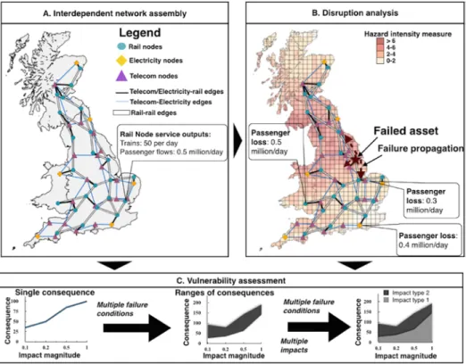
The vulnerability assessment framework developed in this study is illustrated in Figure 1. The framework is divided into components that combine to provide coherent vulnerability assessment outcomes. As is evident, there exists a workflow of model implementation in the Figure 1 framework. Network disruption analysis in Component B is dependent on Component A network assembly models, and similarly Component C vulnerability assessment calculations follow from Component B disruption analysis. In the sections that follow we provide the mathematical formalization of the vulnerability calculations that produce this framework. We first discuss the vulnerability calculations in Section 2.1, which apply to any generalized understanding of an infrastructure network. Section 2.2 explains how we build and map spatial networks, and utilize their properties to build interdependency relationships that capture combinations of interactions. Following on from this, Section 2.3 describes the mathematical model for estimating disruptions in networks applicable to any generalized understanding of a network. Finally in Section 2.4 we present an implementation of the vulnerability assessment framework, based on the notations developed across Sections 2.1 – 2.3.
Figure 1.Vulnerability assessment framework for national infrastructure networks. 2.1 Vulnerability calculations
For vulnerability calculations we assume that an individual infrastructure asset’s state of
operation is denoted with a state function 𝑟𝑟𝑖𝑖, which can take values in the range [0,1]. In the
current analysis we assume only binary {0,1} values for 𝑟𝑟𝑖𝑖, indicating complete loss of operation
when 𝑟𝑟𝑖𝑖= 0 and all other states of operation when 𝑟𝑟𝑖𝑖= 1. The binary assumption indicates that
we are interested in quantifying catastrophic failure outcomes. For an infrastructure network
comprised of 𝑎𝑎 assets, the state of operation is denoted by the state vector 𝐫𝐫= (𝑟𝑟1, … ,𝑟𝑟𝑎𝑎). Since we
have assigned two possible states of operation to each asset, there are 2𝑎𝑎 possible network state
vectors of which 2𝑎𝑎−1 indicate failures. The comprehensive vulnerability assessment of the
network would involve exploring all negative consequences for the 2𝑎𝑎−1 network states. Since
2𝑎𝑎 could be a very large number, we could also use a sample 𝐫𝐫̅= {𝐫𝐫1, … ,𝐫𝐫𝑏𝑏},𝑏𝑏< 2𝑎𝑎 of possible
states to inform vulnerability analysis.
If the infrastructure network’s state is given by the vector 𝐫𝐫𝑗𝑗, where at least one asset state 𝑟𝑟
𝑖𝑖𝑗𝑗 = 0
indicating failure, then the resulting amount of negative consequences give a measure of the
vulnerability of the network. Since networks are complex systems we need to estimate physical
and functional propagation effects of failures. Here physical and functional propagation effects signify the decrease in the level of network service due to the loss of physical interactions and functional relationships between connected assets in the infrastructure. At present we quantify
the service flow disruption of an individual asset as 𝑆𝑆(𝑟𝑟𝑖𝑖) and assume the generalized network
disruption metric 𝑆𝑆(𝐫𝐫𝑗𝑗) is expressed as 𝑆𝑆�𝐫𝐫𝑗𝑗�=𝑓𝑓(𝑆𝑆�𝑟𝑟
1𝑗𝑗�, … ,𝑆𝑆(𝑟𝑟𝑛𝑛𝑗𝑗)), where 𝑓𝑓() is a function that
estimates the network disruptions from connected asset disruptions. In the next sections we will
develop methods to estimate the function 𝑓𝑓() that take network properties into account.
Network vulnerability is given as a two-dimensional metric that quantifies the following:
• Degree of failure of the network – Measured as the proportion of network assets that have failed due to external shocks or have been randomly removed from the network. If the
network state of operation is given by the vector 𝐫𝐫𝑗𝑗 = (𝑟𝑟
1𝑗𝑗, …𝑟𝑟𝑎𝑎𝑗𝑗) then, under the
as Θ�𝐫𝐫𝑗𝑗�= ∑𝑎𝑎𝑖𝑖=1�1−𝑟𝑟𝑖𝑖𝑗𝑗�
𝑎𝑎 . Θ�𝐫𝐫𝑗𝑗� is a normalized global measure of networks’ physical integrity
to shocks as Θ�𝐫𝐫𝑗𝑗�= 1 indicates the network is fully physically intact and operational,
while Θ�𝐫𝐫𝑗𝑗�= 0 indicates the network has totally failed.
• Relative magnitude of negative consequences of disruption – Measured as the ratio between the service disruption following failure and the service level before failure. If pre-disruption
the network delivers 𝑆𝑆 amount of service and in the state 𝐫𝐫𝑗𝑗 it suffers a service loss of
amount 𝑆𝑆(𝐫𝐫𝑗𝑗), then the relative magnitude of negative consequences of disruption is
expressed as Φ�𝐫𝐫𝑗𝑗�= 1−𝑆𝑆(𝐫𝐫𝑗𝑗)
𝑆𝑆 . Φ�𝐫𝐫𝑗𝑗� is a normalized global measure of networks’
increased functional vulnerability to shocks as Φ�𝐫𝐫𝑗𝑗�= 1 indicates the network is fully
functional, while Φ�𝐫𝐫𝑗𝑗�= 0 indicates the network has lost all functionality.
Combining the above expressions, Equation (1) explains the vulnerability metric 𝑉𝑉�𝐫𝐫𝑗𝑗� for the
network state vector 𝐫𝐫𝑗𝑗.
𝑉𝑉�𝐫𝐫𝑗𝑗�=�Θ�𝐫𝐫𝑗𝑗�,Φ�𝐫𝐫𝑗𝑗��=�∑𝑎𝑎𝑖𝑖=1�1−𝑟𝑟𝑖𝑖𝑗𝑗�
𝑎𝑎 , 1−
𝑆𝑆(𝐫𝐫𝑗𝑗)
𝑆𝑆 � (1)
Since both components of the vulnerability metric are normalized we can compare different types of negative consequence outcomes over a wide variety of impacts and performance metrics. By assembling multiple vulnerability measures for different network state vectors sampled from the
set 𝐫𝐫̅, we can generate a comprehensive vulnerability assessment measure
𝑉𝑉(𝐫𝐫̅) =�𝑉𝑉(𝐫𝐫1), … ,𝑉𝑉(𝐫𝐫𝑏𝑏)�, which gives the ranges of possible failure impacts and negative
consequences.
2.2 Network representations and properties
In graph theory, a network is a collection of nodes and edges, where edges represent the connectivity between nodes. In the case of infrastructures edges also represent physical assets
(pipes, cables, road, railway tracks, etc.) that connect nodes. For the infrastructure network of 𝑣𝑣
nodes and 𝑤𝑤 edges (𝑣𝑣+𝑤𝑤=𝑎𝑎) the graph is represented by the set 𝐼𝐼= {𝑁𝑁,𝐸𝐸,𝑀𝑀} comprised of the
node set 𝑁𝑁 = {𝑛𝑛1, … ,𝑛𝑛𝑣𝑣}, edge set 𝐸𝐸 = {𝑒𝑒1, … ,𝑒𝑒𝑤𝑤}, and mapping set 𝑀𝑀 =�𝑒𝑒𝑘𝑘→ �𝑛𝑛𝑦𝑦,𝑛𝑛𝑧𝑧�,∀𝑘𝑘 ∈
[1,𝑤𝑤],𝑦𝑦,𝑧𝑧 ∈[1,𝑣𝑣]�. The arrangement of nodes and edges defined via the mapping set 𝑀𝑀 is called
the topology of the network (Lewis 2011).
Based on their role in facilitating the flow of resources we classify infrastructure network nodes as: (i) source nodes – where the resources are generated; (ii) intermediate nodes – where the resources are transmitted from source nodes towards other nodes; and (iii) sink nodes – where resources are received either directly from source nodes or through the intermediate nodes. A source-sink resource flow lends directionality-based structure to infrastructure networks, thereby providing a complete understanding of interdependence. If a node X receives resources from node Y and vice-versa then X and Y are interdependent even if they are not physically joined by an edge. Such interdependence is possible when there is a functional pathway containing edges and intermediary nodes that have to be physically traversed to get from X to Y (or Y to X). Based on the type of resource flow all source nodes from the network can be extracted and
categorised into separate sets Ω= {Ω1, . . ,Ωc} based on different source types (e.g. Ω = {electricity
substation nodes, railway station nodes, signal tower nodes}, see Section 3.1, Figure 3). For a
single source node 𝑛𝑛𝑜𝑜 selected from the set of all source nodes of a particular infrastructure type
(𝑛𝑛𝑜𝑜∈ Ωl⊂ 𝑁𝑁) and a single sink node 𝑛𝑛𝑠𝑠 selected from the set Λ of all sink nodes (𝑛𝑛𝑠𝑠∈ Λ ⊂ 𝑁𝑁) we
assemble functional pathways between this particular source-sink pair into the set 𝛏𝛏𝑜𝑜∈Ω𝑙𝑙,𝑠𝑠. The
complete pathway set connecting the sink node 𝑛𝑛𝑠𝑠 to all its different source types is represented
by Equation (2).
As there could be multiple functional pathways between a unique source-sink pair, the set
𝛏𝛏𝑜𝑜∈Ω𝑙𝑙,𝑠𝑠 = {𝛏𝛏𝑜𝑜∈Ω𝑙𝑙,𝑚𝑚𝑠𝑠,𝑚𝑚= {1,2 … ,𝑢𝑢}} is produced, assuming 𝑢𝑢 number of paths between the
source-sink pair. Equation (3) shows the mathematical notation for a particular functional pathway (𝛏𝛏𝑜𝑜∈Ω𝑙𝑙,𝑚𝑚𝑠𝑠) when traversing from a single source node to a single sink node.
𝛏𝛏𝑜𝑜∈Ω𝑙𝑙,𝑚𝑚𝑠𝑠= {𝑛𝑛𝑜𝑜,𝑒𝑒𝑧𝑧, … ,𝑒𝑒𝑙𝑙,𝑛𝑛𝑠𝑠} (3)
The existence of multiple functional pathways between source-sink pairs accounts for the
redundancy and robustness of the network structure, as the flow of resources between 𝑛𝑛𝑜𝑜 and 𝑛𝑛𝑠𝑠
stops only if all the pathways in the set 𝛏𝛏𝑜𝑜∈Ω𝑙𝑙,𝑠𝑠 have failed.
2.3 Disruption calculations
In this study disruptions are measured in terms of the ability of the sink nodes to deliver
resources for further consumption. We assume that under normal operations a sink node 𝑛𝑛𝑠𝑠 ∈ Λ
delivers 𝑊𝑊𝑠𝑠 amount of resource, which is delivered along different functional pathways. As
mentioned previously, 𝑊𝑊𝑠𝑠 could represent any performance metric (resource output, customers
served, areas serviced) and there are specific models required to first obtain these metrics. For example in the railway case study we will demonstrate a passenger trip assignment model that is
required to first build 𝑊𝑊𝑠𝑠 estimates. Having mapped the set of functional pathways 𝛏𝛏𝑜𝑜∈Ω𝑙𝑙,𝑠𝑠 =
{𝛏𝛏𝑜𝑜∈Ω𝑙𝑙,𝑚𝑚𝑠𝑠,𝑚𝑚= {1,2 … ,𝑢𝑢}} between a unique source-sink pair, we assume that we can estimate the
contribution of each unique pathway 𝛏𝛏𝑜𝑜∈Ω𝑙𝑙,𝑚𝑚𝑠𝑠 towards the 𝑊𝑊𝑠𝑠 amount of resource delivered as a
weighted fraction 𝛽𝛽𝑜𝑜∈Ω𝑙𝑙,𝑚𝑚𝑠𝑠∈[0,1] of 𝑊𝑊𝑠𝑠. The weight set 𝛃𝛃𝑜𝑜∈Ω𝑙𝑙,𝑠𝑠=�𝛽𝛽𝑜𝑜∈Ω𝑙𝑙,1𝑠𝑠, … ,𝛽𝛽𝑜𝑜∈Ω𝑙𝑙,𝑚𝑚𝑠𝑠� shows the
relative contribution of all pathways between each source-sink pair and for all sources of a
particular infrastructure type connected to a given sink node 𝑛𝑛𝑠𝑠, ∑∀𝑜𝑜∈Ω𝑙𝑙∑𝑢𝑢𝑖𝑖=1𝛽𝛽𝑜𝑜∈Ω𝑙𝑙,𝑚𝑚𝑠𝑠= 1. Similar
to different pathway sets connecting the sink node 𝑛𝑛𝑠𝑠 to all its different source types represented
by Equation (3), we can construct different weight sets as given in Equation (4).
𝛃𝛃𝑠𝑠 = �𝛃𝛃∀𝑜𝑜∈Ω1,𝑠𝑠, … ,𝛃𝛃∀𝑜𝑜∈Ω𝑐𝑐,𝑠𝑠� (4)
As is evident from Equation (4), we have assigned different weights for sources belonging to each infrastructure type, which also means the weights have different interpretations. If the source and
sink infrastructure types are the same then 𝛽𝛽𝑜𝑜∈Ω𝑙𝑙,𝑚𝑚𝑠𝑠 is the fraction of resources being delivered
towards sink output, whereas if the source and sink infrastructure types are different then
β𝑜𝑜∈Ω𝑙𝑙,𝑚𝑚𝑠𝑠 is a measure of the influence the source resource has on the sink output. For example, in
a railway network if 1000 passengers reach a station from two routes such that 600 arrive from
one and 400 from another then 𝛃𝛃∀𝑜𝑜∈Rail,𝑠𝑠 = {3/5,2/5} shows the proportions of passengers
arriving from the different routes. If the same railway station also requires electricity from two separate substation sources providing 200 Gwh/day and 100 Gwh/day respectively then
𝛃𝛃∀𝑜𝑜∈Electricity,𝑠𝑠 = {2/3,1/3} shows the proportions of electricity supplies from the sources required
to operate the railway station.
When disrupted by external shocks, some of the source-sink functional pathways may no longer be operational due to failure of nodes and edges. Following the disruptive impact we assign a
binary state 𝜌𝜌𝑜𝑜∈Ω𝑙𝑙,𝑚𝑚𝑠𝑠∈[0,1] function to each unique path 𝛏𝛏𝑜𝑜∈Ω𝑙𝑙,𝑚𝑚𝑠𝑠∈ 𝛏𝛏𝑜𝑜∈Ω𝑙𝑙,𝑠𝑠,𝑚𝑚= {1, … ,𝑢𝑢}, where
𝜌𝜌𝑜𝑜∈Ω𝑙𝑙,𝑚𝑚𝑠𝑠= 1 implies that the pathway is still in operation and 𝜌𝜌𝑜𝑜∈Ω𝑙𝑙,𝑚𝑚𝑠𝑠= 0 means the pathway has
failed. 𝜌𝜌𝑜𝑜∈Ω𝑙𝑙,𝑚𝑚𝑠𝑠 is a function of the network state vector 𝐫𝐫 because the pathway’s functionality
depends upon its included assets. The post-disruption service level output of a sink node 𝑛𝑛𝑠𝑠
depending upon source nodes of a particular infrastructure type Ω𝑙𝑙 in the disruption state 𝐫𝐫𝑗𝑗 is
given as
𝑊𝑊Ω𝑗𝑗𝑙𝑙,𝑠𝑠 =∑∀𝑜𝑜∈Ω𝑙𝑙∑𝑚𝑚=1𝑢𝑢 max�0,𝜌𝜌𝑜𝑜∈Ω𝑗𝑗 𝑙𝑙,𝑚𝑚𝑠𝑠� 𝛽𝛽𝑜𝑜∈Ω𝑙𝑙,𝑚𝑚𝑠𝑠𝑊𝑊𝑠𝑠 (5)
Equation (5) provides the values for the disruption effects for one type of sources supplying resources to the sink node. Similar estimates can be obtained over different source types
connected to the sink 𝑛𝑛𝑠𝑠 to assemble the set �𝑊𝑊Ω𝑙𝑙,𝑠𝑠
𝑗𝑗 ,∀Ω
output of a sink node is the minimum of the service outputs 𝑊𝑊Ω𝑗𝑗𝑙𝑙,𝑠𝑠 for each category of sources it depends upon, and is given by Equation (6) below.
𝑊𝑊(𝑟𝑟𝑠𝑠𝑗𝑗) = minΩ𝑙𝑙∈Ω{𝑊𝑊Ω𝑙𝑙,𝑠𝑠
𝑗𝑗 } (6)
The service loss, introduced in Section 2.1, at the sink node is the difference between the
pre-disruption and post-pre-disruption estimates of service, i.e. 𝑆𝑆�𝑟𝑟𝑠𝑠𝑗𝑗�= 𝑊𝑊𝑠𝑠− 𝑊𝑊(𝑟𝑟𝑠𝑠𝑗𝑗). If there are 𝜍𝜍
number of sink nodes for which we are estimating the service delivery post-disruption then the total network post-disruption service output is calculated by summing up the individual disruptions at the sink nodes, as explained in Equation (7). Since a sink node signifies the final point of delivery for further usage of the resource, we are assuming that the outputs across sink nodes are discrete and hence add up to give final post-disruption outputs.
𝑆𝑆(𝐫𝐫𝑗𝑗) =∑ �𝑊𝑊
𝑠𝑠− 𝑊𝑊(𝑟𝑟𝑠𝑠𝑗𝑗)� 𝜍𝜍
𝑠𝑠=1 (7)
The functional vulnerability metric in Section 2.1 is derived from the pre- and post-disruption
service outputs as Φ�𝐫𝐫𝑗𝑗�= 1−∑𝜍𝜍𝑠𝑠=1�𝑊𝑊𝑠𝑠−𝑊𝑊(𝑟𝑟𝑠𝑠𝑗𝑗)�
∑𝜍𝜍𝑠𝑠=1𝑊𝑊𝑠𝑠 . The application of the disruption estimation on
actual networks is further explained for the railway case study presented in Sections 3 and 4.
2.4 Vulnerability assessment algorithm
Table 1 below summarises the algorithm for implementing the vulnerability assessment methodology outlined in Sections 2.1 – 2.3, and shown in Component C of Figure 1. The algorithm is implemented using an appropriate programming tool. In this study we have developed and implemented all models using the Python programming language (Van Rossum, 1993). This allowed us to use inbuilt libraries and functions and also create new functions for performing calculations on spatial networks.
Step 3 of the algorithm, where the failure state 𝐫𝐫j is generated, is implemented via Monte Carlo
simulation based on sampling from the set of assets that are considered vulnerable due to exposure to the hazard. By using random seed generators we can obtain different failure combinations of all vulnerable assets and assign appropriate failure states (0 or 1) to them.
Algorithm to simulate the network failures and vulnerability calculations.
Table 1.
1. Network Assembly:
Topological network with source (𝛀𝛀) - sink (𝚲𝚲) directionality and flows Sink node set Λ = {𝑛𝑛1, … ,𝑛𝑛𝜍𝜍} with demands
Resource delivery outputs 𝑊𝑊=�𝑊𝑊1, … ,𝑊𝑊𝜍𝜍� 2. Network path flow analysis:
Assemble all source-sink paths ∀𝑜𝑜 ∈ Ω,𝑠𝑠 ∈ Λ For each sink find 𝛏𝛏𝑠𝑠= �𝛏𝛏∀𝑜𝑜∈Ω1,𝑠𝑠, … ,𝛏𝛏∀𝑜𝑜∈Ω𝑐𝑐,𝑠𝑠�
For each sink estimate path weights 𝛃𝛃𝑠𝑠= �𝛃𝛃∀𝑜𝑜∈Ω1,𝑠𝑠, … ,𝛃𝛃∀𝑜𝑜∈Ω𝑐𝑐,𝑠𝑠�
3. Shock-network intersection: Assemble failure set 𝐫𝐫j 4. Residual path analysis:
Remove all assets 𝑖𝑖, s.t. 𝑟𝑟𝑖𝑖𝑗𝑗∈ 𝐫𝐫𝑗𝑗,𝑟𝑟
𝑖𝑖𝑗𝑗= 0 and their paths
For each sink assemble the path state set 𝛒𝛒𝑠𝑠= �𝛒𝛒∀𝑜𝑜∈Ω1,𝑠𝑠, … ,𝛒𝛒∀𝑜𝑜∈Ω𝑐𝑐,𝑠𝑠�
5. Assemble sink failure estimates: Find 𝑊𝑊(𝑟𝑟𝑖𝑖𝑗𝑗) from Equations (5) and (6) 6. Calculate impact magnitude: Find Θ(𝐫𝐫j)
Calculate disruption estimates: 𝑆𝑆(𝐫𝐫𝑗𝑗) from Equation (7) Calculate vulnerability metric: 𝑉𝑉(𝐫𝐫𝑗𝑗) from Equation (1)
3.
Case-study for Great Britain’s railway infrastructure
This section describes the application of the methodology developed in Section 2 to the railway network for Great Britain, which is a critical infrastructure. Railway passenger usage in Great Britain has increased by a quarter over the last five years, and an estimated 1.5 billion journeys totalling 36 million miles were made on the railway network during 2012-2013, which was double the number of journeys made in 1994-1995 (Department for Transport, 2013b). Over the next few years substantial investment is planned both to construct new routes and to upgrade existing railway infrastructure (HM Treasury, 2013; Network Rail, 2014). There have though been several instances of serious failures that have highlighted the vulnerability of the railway infrastructure, showing the need both for additional investments and for a better understanding of the risks facing the network. The Great Britain rail network experienced about 3 million train delay minutes in 2007 due to weather related external shocks (Dobney et al., 2009). Widespread flooding between December 2013 and February 2014 resulted in an estimated £100m of damage to the railway infrastructure, requiring around 4000 railway staff to be constantly deployed to tackle flood water and repair infrastructure to keep trains running (Topham, 2014).
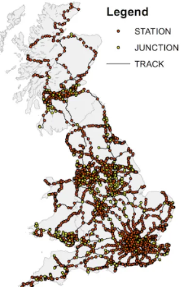
Figure 2 shows the spatial and topological representation of Great Britain’s railway network, which was assembled from a combination of datasets provided by Ordnance Survey (Ordnance Survey, 2013), the Association of Train Operating Companies (ATOC) (ATOC, 2013), and the Department for Transport (the National Public Transport Access Node database (NaPTAN)) (Department for Transport, 2013a). The network consists of 3959 nodes and 4457 edges. Network nodes represent stations (2539 nodes) and junctions (1420 nodes), while edges represent all routes between nodes. Demand assignments in the railway network are quantified in terms of the average daily passenger trip flows across network nodes and edges, which are shown in Figure 3. Section 3.1 outlines the detailed trip assignment methodology developed in this study to generate these results. Since modern day railway networks are comprised of several complex subsystems that make them functional, there are other assets that we need to include in the network representation of an interdependent railway infrastructure. In particular, other infrastructures such as electricity, water, telecommunications (ICT), gas and fuels have an influence of railway operations. In Section 3.2 we discuss some of these assets that exist in the railway infrastructure, while in Section 3.3 we explain how these assets are mapped to the network to create physical and functional interdependencies.
Figure 2.Topological railway network for Great
Britain showing stations, junctions and tracks. Figure 3.analysis showing estimates of daily number of Results of the railway trip assignment passenger trips across individual railway network edges (track sections).
3.1 Trip assignment and disruption modelling for railways
We are interested in quantifying the negative consequences for passenger travel resulting from disruptions at stations, junctions or track sections in the railway network. At any given time the railway network is being used by people to travel from one location to another, which creates passenger trip measures along the network. Hence we develop estimates of passenger-trips lost when the network is disrupted due to external shocks.
As a starting point we require some means of estimating the number of passengers travelling along a given section of railway route or through a given station during a certain time period. While extensive research has been carried out into rail demand forecasting in Great Britain (Department of Transport, 2009; Worsley, 2012), the data and outputs relating to these models were either: (i) not available for reasons of commercial confidentiality; or (ii) only relate to aggregated trips at individual stations or between zones, and therefore do not assign trips to particular segments of route.
We therefore developed a method for estimating trip assignment to the railway network based on the limited datasets that are available, focusing particularly on the Office of Rail Regulation’s (ORR) station usage dataset. These provide details of the annual number of passengers entering, exiting and interchanging at all individual railway stations in Great Britain (ORR, 2013). This is complemented by electronic timetable data available from the Association of Train Operating Companies (ATOC), which gives full details of routing and calling points for all passenger trains operating on the Great Britain rail network over the period of validity of the timetable (ATOC, 2013). A set of Python functions were written to match the electronic timetable information with the spatial network (Figure 2), in order to create specific geocoded route information for each train journey. The trip assignment model calculations, which give the daily number of passenger trips between stations along specific routes, are explained in the subsections that follow.
Trip generation and attraction
The first step in the trip assignment model involves estimating the number of trips generated and attracted at all individual stations on the railway network. Since every station is a point of passenger entry or exit in the railway network, it is both a source and a sink. Here as is conventional in transport modelling we use the terms origin (source) and destination (sink). We calculated the daily number of passengers using stations by first converting the annual station usage figures (ORR, 2013) into weekly estimates, and then allocating the weekly estimates to particular days in proportion to the train frequencies for each day. The respective calculations for
number of entries (𝜂𝜂𝑠𝑠𝑑𝑑) and number of exits (𝜅𝜅𝑠𝑠𝑑𝑑) at a station (𝑠𝑠) on a given day (𝑑𝑑) are shown in
Equations (8) and (9). 𝑄𝑄𝑠𝑠 is the annual number of entries plus interchanges, and 𝐻𝐻𝑠𝑠 is the annual
number of exits plus interchanges at the station 𝑠𝑠. Interchanges occur when passengers change
trains during their journeys, and hence were accounted for in both the entries and exits calculations. It is assumed that passenger numbers are distributed equally over all weeks of the year, as while in practice there will be some variation based on (for example) holiday periods, no data were available which allowed such variation to be quantified. In estimating the trip distribution across the week we calculated the daily number of trains at each station as being a
combination of the number of trains starting (passengers only enter) (𝑡𝑡𝑠𝑠st,𝑑𝑑), making intermediate
stops (passengers enter and exit) (𝑡𝑡𝑠𝑠in,𝑑𝑑) or terminating (passengers only exit) (𝑡𝑡𝑠𝑠te,𝑑𝑑) at the station.
𝜂𝜂𝑠𝑠𝑑𝑑 =𝑄𝑄52𝑠𝑠� 𝑡𝑡𝑠𝑠 st,𝑑𝑑+𝑡𝑡 𝑠𝑠in,𝑑𝑑 ∑𝑑𝑑(𝑡𝑡𝑠𝑠st,𝑑𝑑+𝑡𝑡𝑠𝑠in,𝑑𝑑)� (8) 𝜅𝜅𝑠𝑠𝑑𝑑=52𝐻𝐻𝑠𝑠� 𝑡𝑡𝑠𝑠 te,𝑑𝑑+𝑡𝑡 𝑠𝑠in,𝑑𝑑 ∑𝑑𝑑(𝑡𝑡𝑠𝑠te,𝑑𝑑+𝑡𝑡𝑠𝑠in,𝑑𝑑)� (9)
Trip distribution and assignment
The second step in the trip assignment model involves matching the total trip origin and destination information calculated in the previous section to create an origin-destination (O-D)
trip matrix, while simultaneously allocating these trips to the rail network. The aggregate daily station usage figures estimated using Equations (8) and (9) were converted to flows along specific
paths using Equations (10) and (11). These allow estimation of the number of passenger trips 𝜇𝜇𝑂𝑂𝑂𝑂𝑃𝑃,𝑑𝑑
made between an origin (𝑂𝑂) and destination (𝐷𝐷) using a particular rail service (path 𝑃𝑃) for each
day𝑑𝑑. The steps of the trip assignment calculations are explained as follows:
1. The number of entries (𝜂𝜂𝑂𝑂𝑑𝑑) indicate the volume of flow that has to be directed from the
origin station along specific paths. The timetable data (ATOC, 2013) gives us information
on rail service paths, where a path (𝑃𝑃) for each station is defined as a unique route across
the network taken by trains calling at that station. For each path 𝑃𝑃 we calculate a trip
attractiveness factor (𝑓𝑓𝑂𝑂𝑃𝑃,𝑑𝑑) in relation to the entry station 𝑂𝑂, which is the product of the
number of trains along the path from station 𝑂𝑂 (𝑡𝑡𝑂𝑂𝑃𝑃,𝑑𝑑) and the total volume of exiting
passengers (∑𝑂𝑂∈𝒟𝒟𝑂𝑂𝑃𝑃𝜅𝜅𝑂𝑂𝑑𝑑) at all stations (𝒟𝒟𝑂𝑂𝑃𝑃) along the path beyond station 𝑂𝑂. The trip
attractiveness factor is used to determine how the aggregated volume of flow from the
entry station is directed over the course of the day along path 𝑃𝑃, based on the volumes of
trains and station exits along different paths. At each station where passengers can enter a
path, we convert the station entry estimates into trip entry estimates (𝜂𝜂𝑂𝑂𝑃𝑃,𝑑𝑑) by dividing
(𝜂𝜂𝑠𝑠𝑑𝑑) between the available paths in proportion to the trip attractiveness factors, as shown
in Equation (10). The paths with higher trip attractiveness factors will therefore attract more passengers from the entry station over the course of the day.
2. The trip entry estimates for each path are then used to calculate a set of O-D flow
estimates𝜇𝜇𝑂𝑂𝑂𝑂𝑃𝑃,𝑑𝑑 (Equation (11)), which give the number of trips made between an O-D pair
using a particular path. We assume that along a path the number of passengers getting
off at a station is in direct proportion to the station’s total trip exits (𝜅𝜅𝑠𝑠𝑑𝑑) relative to other
stations along the path. Aggregated over the day, a station with a larger number of total exits (plus interchanges) will see a proportionally greater number of passengers alighting from every train that calls there.
𝜂𝜂𝑂𝑂𝑃𝑃,𝑑𝑑 =𝜂𝜂𝑂𝑂𝑑𝑑
�
𝑡𝑡𝑂𝑂 𝑃𝑃,𝑑𝑑∑ 𝜅𝜅 𝐷𝐷 𝑑𝑑 𝐷𝐷∈𝒟𝒟𝑂𝑂𝑃𝑃 ∑ �𝑃𝑃 𝑡𝑡𝑂𝑂𝑃𝑃,𝑑𝑑∑𝐷𝐷∈𝒟𝒟𝑂𝑂𝑃𝑃𝜅𝜅𝐷𝐷𝑑𝑑��
=𝜂𝜂𝑂𝑂 𝑑𝑑�
𝑓𝑓𝑂𝑂𝑃𝑃,𝑑𝑑 ∑𝑃𝑃𝑓𝑓𝑂𝑂𝑃𝑃,𝑑𝑑�
(10) 𝜇𝜇𝑂𝑂𝐷𝐷𝑃𝑃,𝑑𝑑 =𝜂𝜂 𝑂𝑂 𝑃𝑃,𝑑𝑑�
𝜅𝜅𝐷𝐷𝑑𝑑 ∑𝐷𝐷∈𝒟𝒟𝑂𝑂𝑃𝑃𝜅𝜅𝐷𝐷𝑑𝑑�
(11)The above calculations conserve the total number of flows along each path, because they guarantee that the total of the O-D flow estimates equals the total of all entries made in the path. This is explained mathematically by Equation (12).
∑ ∑𝑂𝑂 𝑂𝑂∈𝒟𝒟𝑂𝑂𝑃𝑃𝜇𝜇𝑂𝑂𝑂𝑂𝑃𝑃,𝑑𝑑 =∑ ∑ 𝜂𝜂𝑂𝑂𝑃𝑃,𝑑𝑑� 𝜅𝜅𝐷𝐷 𝑑𝑑 ∑ 𝜅𝜅𝐷𝐷𝑑𝑑 𝐷𝐷∈𝒟𝒟𝑂𝑂𝑃𝑃 � 𝑂𝑂∈𝒟𝒟𝑂𝑂𝑃𝑃 𝑂𝑂 =∑ 𝜂𝜂𝑂𝑂 𝑂𝑂𝑃𝑃,𝑑𝑑 (12)
Relating to the resource output metrics introduced in Section 2.3, the two equations, 𝑊𝑊𝑂𝑂=
∑ ∑ 𝜇𝜇∀𝑃𝑃 ∀𝑂𝑂 𝑂𝑂𝑂𝑂𝑃𝑃,𝑑𝑑 and 𝜇𝜇𝑂𝑂𝐷𝐷 𝑃𝑃,𝑑𝑑
𝑊𝑊𝐷𝐷 =𝛽𝛽𝑂𝑂∈Ω𝑙𝑙,𝑚𝑚𝑂𝑂,Ω𝑙𝑙= {Railway Station}, can be derived. For a given destination
(sink) station 𝐷𝐷 all the O-D flow estimates add up to give the amount of trips completed, i.e.,
resources delivered; hence they add up to the metric 𝑊𝑊𝑂𝑂. Also each 𝜇𝜇𝑂𝑂𝑂𝑂𝑃𝑃,𝑑𝑑 indicates the value of
flow along each individual O-D pathway and proportionally gives the pathway weight metric
𝛽𝛽𝑂𝑂∈Ω𝑙𝑙,𝑚𝑚𝑂𝑂.
The O-D flow estimates developed here are static estimates for the average daily flows through the railway network calculated using freely available data. While the assumptions made when assigning trips to paths mean that the methodology may not exactly reproduce actual travel behaviour, they should provide an approximation that is accurate enough for the purposes of this study (i.e. disruption estimation).
3.2 Mapping key critical components for railways
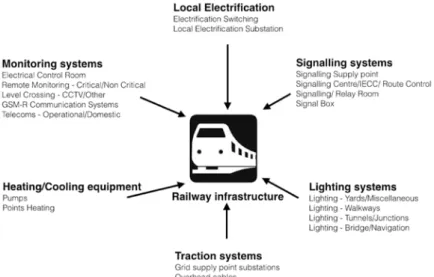
We have compiled a list of some of the key critical components (assets) that are responsible for cross-infrastructure interdependencies in an operational railway network in Great Britain. This list reflects our understanding of the railway infrastructure and also results from data provided by Network Rail, who are the owners and operators of the rail infrastructure in Great Britain. Based on our interpretation of similarities in functionality the following six broad categories of assets emerge: (i) electrification equipment, (ii) signalling systems, (iii) monitoring systems, (iv) lighting systems, (v) heating and cooling systems, and (vi) traction systems. These are shown in Figure 4. While this is not an exhaustive list, all railway operations at stations, junctions and along tracks are dependent on these assets. Since Great Britain’s railway network operates on similar standards to other European and worldwide networks, the asset list compiled here can be used to study other similar railway infrastructures.
Figure 4.Different components of the railway network.
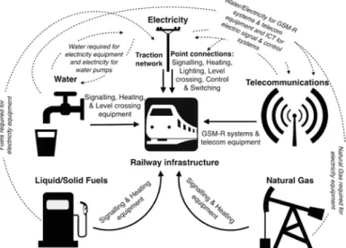
As is evident from Figure 4, the railway network requires resources from other infrastructures for operating assets. Figure 5 shows the key infrastructures that supply the resources for operating the assets listed in Figure 4. We have mapped key interdependencies between infrastructures based on the operational requirements of assets. Some of the infrastructures supply resources directly to the railway network, which results in a direct mapping between the infrastructures. In Figure 5 the solid black arrows represent such mapping. In most cases there is more than one layer of interdependent mapping, where a railway asset requires resources from different infrastructures in order to operate. In Figure 5 the dashed black arrows represent such indirect mappings. The direction of the arrows in each mapping shows the direction of resource flows across infrastructures, which helps in building the network functional pathways (discussed further in Section 3.2).
Figure 5.Interdependency mappings between infrastructures that are required for an operational railway network.
3.3 Network representations of key critical component interdependencies
We first identified the locations of the key critical components (assets) from Figure 4 to integrate them in the spatial railway network shown in Figure 2. We note that other infrastructure networks (e.g. electricity transmission grid, water supply network, etc.) have not been included here, rather we are inferring their interdependence and influence on the railway infrastructure through the assets listed in Figure 4. All assets were interpreted as network nodes whose spatial coordinates were either available in the data or built using other asset information which was processed using Python functions. For example, functions were written to convert postcode and Ordnance Survey grid information into coordinates and to extract location information from Open Street Map via the address information for the asset. After populating the raw data with relevant spatial information a dataset containing 8347 point assets (excluding the station and junction nodes in the Figure 2 network) was created for this study.
Since each asset in Figure 4 supplies resources to the railway network, it is designated as a source
node and belongs to the set Ω, while the sink node set Λ contains the stations and junctions.
Physically all these sources were joined to their nearest edge (track) or node (station or junction) by single-line geometries. Functionally some assets supply resources only to the sink nodes or
edges they are directly connected to, which means the functional pathway 𝛏𝛏𝑜𝑜∈Ω𝑙𝑙,𝑚𝑚𝑠𝑠 includes just
the source and sink. This is shown in Figure 6 through a graphical representation where assets such as points heating, lighting systems, and level crossing equipment influence only the railway node or edge they are directly connected to. Other assets supply resources or influence a significant proportion of the railway network. For example in Figure 6 the traction system consists of electricity substations (grid supply point station) that supply to groups of stations, junctions and their related tracks. In reality the substation supplying electricity to the traction system is connected to its nearest node on the railway network via an overhead cable, which is then connected to the next station via another cable to branch out the electricity supply. This is shown in Figure 6. Similarly, many signalling and telecommunication systems influence the operation of multiple stations, junctions and tracks and are connected in a similar way. In most cases the railway networks are divided into specific strategic routes (a collection of stations) that have operational boundaries. This information is used while assigning functional pathways for the traction, signalling and telecommunication systems. For example we know that certain routes of the British railway network (e.g. East Coast Main Line, Great Western Line) are operated by single IECC (Integrated Electronic Control Centre) systems, and we used this information to create functional pathways in the railway network.
Figure 6.Illustration of functional (topological and operational) connectivity of certain assets to the railway network. Assets such as level crossings, signalling points or point heating are connected to their nearest node (station/junction) or edge. Assets such as traction electricity substations are connected to their nearest node and through overlaying a series of overhead cables along the network the electricity is supplied to other stations.
Certain redundancies also exist in the railway infrastructure, which we accounted for in the functional mapping. In particular if a grid supply point substation in the traction system shuts down due to failures its supply is replaced by adjacent substations. Hence for each station, junction or track that is electrified, functional pathways to every adjacent grid supply point were mapped.
We assume here that if a sink is connected to multiple sources of the same type only one of them is operation at one time and the rest are for backup supply. This implies that we are assigning
weights 𝛽𝛽𝑜𝑜∈Ω𝑙𝑙,𝑚𝑚𝑠𝑠= 1 to all functional pathways that exist between source types listed in Figure 3.
Hence we assume here that every asset is critical for the functioning of the railway infrastructure, and unless there are backups the associated sink nodes stop operating once the sources fail. Evidence suggests that railway operations are halted temporarily when the type of assets listed here fail until they can be repaired (Network Rail 2014).
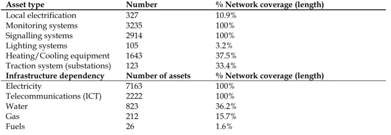
Table 2 gives information (derived from the asset dataset) on the number of assets belonging to the different infrastructure types (shown in Figure 4) and their spatial coverage (% length) on the railway network. It is clear that the railway infrastructure is most dependent upon electricity and telecommunication infrastructures, followed by water, natural gas and fuels. Based on asset types monitoring and signalling systems have influence over the largest proportion of the network compared to other asset types. The percentage spatial coverage values can also be used as indicative metrics for quantifying vulnerability as they provide an indication of the extent of damage to the railway infrastructure resulting from widespread failures in other assets and infrastructures.
List of asset numbers and spatial coverage divided by asset types and infrastructure
Table 2.
types that supply resources to the railway infrastructure.
Asset type Number % Network coverage (length)
Local electrification 327 10.9%
Monitoring systems 3235 100%
Signalling systems 2914 100%
Lighting systems 105 3.2%
Heating/Cooling equipment 1643 37.5%
Traction system (substations) 123 33.4%
Infrastructure dependency Number of assets % Network coverage (length)
Electricity 7163 100%
Telecommunications (ICT) 2222 100%
Water 823 36.2%
Gas 212 15.7%
4.
Vulnerability assessment results and insights
In the current analysis we are interested in evaluating the railway network vulnerabilities due to interdependent failures initiated in the six different assets types presented in Section 3.1.
We look at the propagation of interdependent asset failures towards railway operation disruptions, depending upon connectivity to nodes (stations or junctions) or edges (tracks). In both instances disruption effects extend up to the nearest nodes where the trains can still operate. Following disruption each path is therefore ‘broken’ into separate sections along which trains are still operational. We assume day long disruption scenarios for every failure outcome and estimate the pre- and post-disruption trips for that day. If the disruption occurs for more than a day then we can estimate the flow damages over the entire time period since we have daily estimates of origin-destination flows. We note that here flow rerouting, congestion and other trip reassignment mechanisms are not considered. We acknowledge that in reality rerouting should be considered as it has a considerable effect on failure estimates, but to some extent this can be relaxed for railway networks because large sections of the railway network have very limited diversionary options. We are measuring the worst-case negative consequences for each disruption, which for widespread failure could be very plausible. In the calculations we estimate the post-disruption passenger trips for all existing O-D pairs and sum them to get the overall
network flow, i.e., 𝑊𝑊�𝐫𝐫𝑗𝑗�=∑ ∑ ∑ max�0,𝜌𝜌
𝑂𝑂,𝑃𝑃𝑂𝑂𝑗𝑗 � 𝜇𝜇𝑂𝑂𝑂𝑂𝑃𝑃,𝑑𝑑 ∀𝑂𝑂
∀𝑃𝑃
∀𝑂𝑂 . The passenger trip loss estimates
follow from Equation (7).
We consider the results from two types of vulnerability assessment results, firstly random component failures and secondly flood vulnerability.
4.1 Random component failures
We test the vulnerability of the railway network due to random failures of different sets of interdependent assets selected using two criteria.
1. Criteria 1 – We choose assets based on their functionality as defined through the six
categories in Figure 3. Separate calculations are done for each asset category, where it is assumed only those assets of the chosen category fail. Hence the vulnerability assessment tests the criticality of each type of supporting asset in the railway infrastructure.
2. Criteria 2 – We choose assets based on the type of infrastructure that is supplying the
resources to make them operational. The five infrastructure types shown in Figure 4 are selected individually and we test failure sets for them separately. Here the vulnerability assessment tests the criticality of the dependence of the railway infrastructure on other infrastructures.
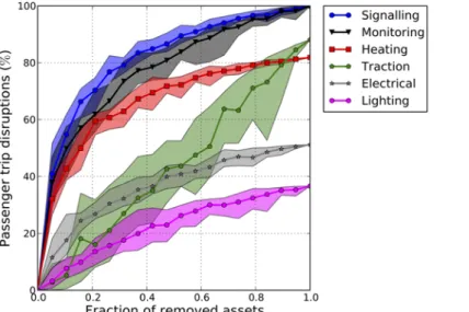
Figure 7 shows the vulnerability assessment results when assets are chosen according to Criteria 1 and different degrees of random failures are introduced in the railway infrastructure network. The x-axis shows the number of each asset type that is removed for the network, expressed as a
fraction of its total number in the network, which is the metric Θ�𝐫𝐫𝑗𝑗� introduced in Section 2.1.
The y-axis shows the daily loss of passenger trips over the entire network expressed as a
percentage of pre-disruption passenger trip estimates, which is the metric Φ�𝐫𝐫𝑗𝑗� expressed as a
percentage. To generate the Figure 7 results we implemented 250 simulations for each magnitude of random failure scenario in order to capture the full range of vulnerability outcomes. The size of the railway network governs the number of simulation runs, because each trip disruption loss estimate is produced by recalculating the trips on the disrupted network, which is computationally expensive. Our aim here is to show a substantial range of possible vulnerability outcomes to demonstrate the methodology.
The results in Figure 7 show that railway systems are vulnerable to equipment failures in the following order (high to low): (i) signalling systems, (ii) monitoring systems, (iii) heating systems, (iv) traction systems, (v) electrical (local) systems, and (vi) lighting systems. These results are
influenced by three factors: (i) the quantity and spatial coverage of the assets (see Table 2); (ii) the location on the network where the assets are installed; and (iii) the network flows through the parts of the network supported by the assets. Apart from traction systems all other asset vulnerabilities grow at almost similar rates because of the comparable spatial coverage of individual assets. Even though the heating systems (point heating) cover only 37.5% of the network (see Table 2), they have a significant impact on network operations because they are installed strategically along the busiest routes of travel. In the case of traction systems, since each grid supply substation supplies to multiple nodes, progressive failures lead to much larger impacts compared to other systems. Also, even though there are fewer assets (substations) in the traction system over a smaller spatial proportion of the network (33.4%, see Table 2), they supply power to most of the busiest routes (in terms of passenger flow) resulting in larger disruptive impacts.
Figure 7.Vulnerability of the railway network due to random failures of different type of functional assets.
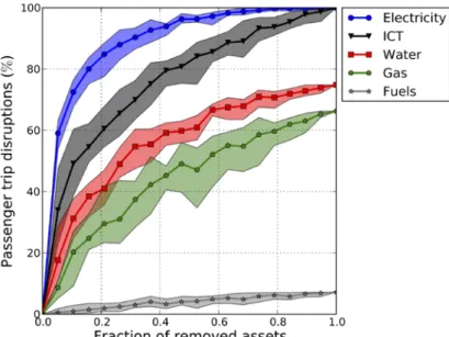
Figure 8 shows the vulnerability assessment results when assets are chosen according to Criteria 2 and different degrees of random failures are introduced in the railway infrastructure network. The axes in Figure 8 are similar to the ones in Figure 7, and the results are again generated following 250 simulation runs per failure magnitude. The results in Figure 8 show that railway infrastructure is most vulnerable to other infrastructure failures in the following order (high to low): (i) electricity, (ii) telecommunications (ICT), (iii) water, (iv) natural gas, and (v) liquid/solid fuels. These results are in line with expectations given the number of assets that require electricity and ICT for their operations.
Figure 8.Vulnerability of the railway network due to failures induced through other infrastructures. 4.2 Flood vulnerability
As with the random failure scenarios, the flood vulnerability of the railway infrastructure is tested with respect to failures to critical assets. In particular flood vulnerability is evaluated here in terms of the likelihood of exposure to floods and the resultant negative consequences.
We have used the National Flood Risk Assessment (NaFRA) flood likelihood map for England and Wales, which is illustrated for a localized area in Figure 9 (Environment Agency, 2009). The map data provides information on the estimated likelihood of flooding to areas of land within the flood plain of an extreme flood (0.1 per cent or 1 in 1000 chance of fluvial and/or tidal flooding in any year). The likelihood of flooding takes in account the probability that the flood defences will overtop or breach, and the distance of the impact from the river or the sea. The results of the analysis are presented for three flood likelihood risk categories as: (i) low - the chance of flooding each year is 0.5 per cent (1 in 200) or less; (ii) moderate - the chance of flooding in any year is 1.3 per cent (1 in 75) or less but greater than 0.5 per cent (1 in 200); and (iii) significant - the chance of flooding in any year is greater than 1.3 per cent (1 in 75).
Figure 9.Illustration of part of the NaFRA flood likelihood map for England and Wales and its intersection with the railway infrastructure network.
By spatially intersecting the flood likelihood maps with different assets (Figure 9), we generate the list of all assets located in either a low, moderate or significant flood likelihood area. Here it is assumed that the flood protection measures (embankments, raised platforms) around railway
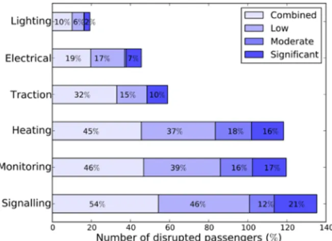
assets are now able to prevent flooding, because we do not have information on such protection standards. The analysis could be improved if such data were made available, and this will form the subject of future work. Hence we perform a worst-case vulnerability assessment by evaluating failure scenarios for assets exposed to flooding. Figure 10 shows the number of different asset types, expressed as percentages of their total numbers, intersecting with the flood areas and belonging to each category of flood risk likelihood. Following the estimate of assets intersecting flood regions, the negative consequences are estimated by assuming four worst-case scenarios where: (i) all assets that intersect with floods fail; and only assets exposed to (ii) low, (iii) moderate or (iv) significant flood risk fail separately. Figure 11 shows the analysis results, where it can be inferred that the heating, monitoring and signalling assets that are flooded have a substantial impact on the railway network. Though not shown here, we can spatially infer that the assets that are exposed to flooding risks are located along some of the busier rail routes, which result in high disruption impacts. For risk management the results show that planning and resource allocation should concentrate on such busy routes. In all cases many assets in areas with low flood likelihoods have large vulnerability impacts if they fail. These results indicate that the low flood risk areas cannot be ignored when risk reduction measures are put in place. For most assets we can derive similar inferences for moderate and significant flood likelihood vulnerability outcomes. The case of traction system vulnerability outcomes again differs from other assets, because when a smaller percentage of traction substations fail they are backed-up by the other substations, whereas such robustness does not exist in other systems.
Figure 10.Flood vulnerability result showing the percentages of different types within each flood likelihood zone.
Figure 11.Flood vulnerability result showing the percentages of disrupted passengers for different type of flood likelihood outcomes.
4.3 Usefulness and development of vulnerability analysis
The winter floods in 2013-2014 in caused major disruptions to Great Britain’s rail network, when large parts of the network were disrupted for extended periods. Several disruptions on the network occurred due to key critical component failures of the type we discussed in this study. Since we have mapped everything spatially we are able to provide Network Rail with information on vulnerability locations and transport corridors. As discussed in Section 1, from Network Rail’s perspective this analysis is very useful towards informing systemic risks and utilising this information to improve network resilience. To make this study of greater use to Network Rail and other railway operators, other asset datasets can be incorporated to create a comprehensive vulnerability and risk assessment tool. These include, among others: (i) Network Rail’s Fault Management System (FMS) dataset which records all key critical component failures and their causes, which can help in creating better strategic and probabilistic failure scenario; (ii) Network Rail asset datasets on flood and other hazard protecting measures, which can provide a better hazard vulnerability assessment; and (iii) Passenger ticketing information datasets that provide data in trips during peak or non-peak hours, which would give better trip disruption estimates.
5.
Conclusions
The work presented in this paper outlines a detailed vulnerability assessment methodology for critical infrastructures at the national scale. We have provided a comprehensive methodology for building spatial railway network models, railway trip assignment models and vulnerability assessment algorithms for national level system failure analysis. We also provide a dataset and template for understanding interdependencies in national-scale railway networks and mapping them spatially, creating a useful tool for infrastructure planners and operators. Through this methodology we have addressed two key issues in building meaningful national scale infrastructure representations, namely: (i) conceptualizing infrastructure network models that capture critical asset characteristics; and (ii) building functionality based interdependency mapping between assets to capture the geographic and operational characteristics of infrastructure networks. The simulation-based approach outlined here highlights the capabilities of the framework to capture multiple vulnerability outcomes and check different failure sensitivities. Overall the framework addresses the requirements of a comprehensive systems performance assessment or impact assessment.
The case study presented here shows a network model representation of Great Britain’s railway infrastructure, which is close to the actual geographic and functional system. Through various datasets we have been able to assemble information on critical railway assets and infer their spatial and functional mapping as best as possible. The analysis provides a template for understanding any modern railway system around the world. We have also presented a railway trip assignment model based on aggregate station usage and service timetable information. The model can be used for present or future railway trip forecasts based on available data. In the vulnerability analysis results for the railway infrastructure the most critical asset impacts are in terms of signalling, monitoring, heating and traction systems, whereas when interdependent infrastructures are considered electricity and telecommunications networks have the biggest impact on railway operations. In the flood vulnerability analysis, we have been able to show that even though there are only a small number of assets exposed to flooding, their impacts on the network functionality are substantial. The vulnerability results highlight the importance of considering: (i) quantity and spatial extents of assets, which influence the spread of failures; and (ii) the specific locations of assets, which influence the disruptions of network flows.
Train operators and planners to identify the locations and sources of vulnerabilities in their networks and plan accordingly can use the detailed analysis of the railway system. Further analysis using this work will lead towards national infrastructure risk analysis and adaptation planning.
Acknowledgements
The authors would like to thank the reviewers for their suggestions towards improving this manuscript. The research reported in this paper was part of the UK Infrastructure Transitions Research Consortium (ITRC) funded by the Engineering and Physical Sciences Research Council under Programme Grant EP/I01344X/1. The authors would also like to thank David Alderson, Research Assistant at The School of Civil Engineering and Geosciences at University of Newcastle (UK) for providing rail network GIS data, and also Network Rail for providing some of their railway utility data.
References
Adger, W. N. (2006). Vulnerability. Global environmental change, 16(3), 268-281.
Albert, R., Jeong, H., & Barabási, A. L. (2000). Error and attack tolerance of complex networks. Nature, 406(6794), 378-382.