DRAFT STATUS UPDATE AND PROPOSAL
http://www.archaeogeophysics.org
An Online Self-Study Resource and Knowledge Management System for the Collection, Processing and Analysis of Archaeogeophysical Data
Prepared for CALTRANS
BY Carl P. Lipo1
Veronica Harper James T. Daniels, Jr.
Tony T. Quach
CALIFORNIA STATE UNIVERSITY LONG BEACH April 30, 2008
1 Department of Anthropology and the Institute for Integrated Research on Materials, Environments and Society
(IIRMES), 1250 Bellflower Blvd, California State University Long Beach, Long Beach, CA 90840,
Table of Contents Introduction... 5 Main Page ... 8 Equipment ... 10 Introduction ... 10 GPR ... 10 Magnetometry ... 11 Resistivity... 11 Conductivity... 12 Techniques ... 13
Ideal Conditions for Geophysics ... 13
GPR ... 14
Magnetometry ... 16
Resistivity... 18
Electromagnetic (EM) Conductivity ... 20
GPS ... 20 Datasets ... 22 Practice sets:... 22 Zzyzx, California SBR-05417... 22 Submitted ... 23 Tutorial Page... 24 Introduction ... 24
Ground Penetrating Radar... 24
Magnetometry ... 30
Magnetometrv Procedures... 30
Resistivity... 35
Conductivity... 41
GPS ... 44
Integrating Geophysical Data in ArcGIS ... 49
Methodology for Integrating Geophysical Data... 49 Software Page ... 56 Introduction ... 56 GPR Slice ... 56 MagMap ... 56 Radan... 56 GeoPlot... 56
Introduction
The integration and analysis of geophysical data for the study of the archaeological record (i.e., archaeogeophysics) is a fast growing and increasingly complex area of field methods development. As new equipment and software become commonly available that permit one to combine data from classes of measurement such as artifact densities, topography, magnetometry, ground penetrating radar, conductivity, global positioning systems, and aerial/satellite imagery, new demands are placed on archaeologists to understand this technology and to learn how data can be assembled into a coherent whole. These technologies have become commonplace in only the last five or so years and consequently are often beyond the training of professionals currently working in field. In addition, not only are archaeologists increasingly expected to understand how to work with multiple datasets consisting of geophysical information, but they are also required to integrate their work with environmental, geological, hydrological, and other kinds of resource managers. This kind of data sharing and management is routinely made possible through the use of geographic information systems (GIS) as a central tool for data set integration and rectification. In sum, expectations for archaeologists have never higher in terms of their ability take classes of information from a wide range of field techniques and merge them with any other kind of dataset for centralized analyses, mitigation evaluation and interpretation.
Training, of course, is required to keep archaeological staff up to speed on new technologies and procedures. Periodic training courses can help in this regard as they allow individuals to take time to refresh themselves with new areas of development in archaeological field research. At CALTRANS, such courses have been run through CSULB and other locations and individuals have been sent to off-site areas for specialized hands-on training. While hands-on courses offer an excellent immersive environment for learning, the information they provide often comes at times long before or after the information is actually needed. In addition, information from the courses may fade in memory before the opportunity comes in the workplace to put new skills to use.
One set of alternatives to in-person courses is an on-line training resource. Usually built as “courseware” or through a “knowledge management” system, on-line training offerings make use of content that users can access at any time and can work through the material at their own pace. While one-to-one interaction is not usually possible in an on-line setting, the ability to continually refer to the material when confronted with real world problems makes on-line
database accessible via the internet, online systems can be continually updated to reflect the latest technology, procedures and information.
One increasingly common means of developing online knowledge management systems is through the use of a wiki. A wiki is a collection of web pages designed to enable any
registered and authorized user who accesses it to contribute or modify content, using a simplified markup language. Wikis are often used to create collaborative websites and to power
community-based websites. For example, the collaborative encyclopedia Wikipedia is one of the best-known wikis. Wikis are commonly used in businesses to provide affordable and effective intranets and for knowledge management. In the context of training in archaeogeophysics, a wiki has the potential to provide a platform for integrating information on the details of
processing and analyzing data with the added benefit of being dynamic so that new information can be incorporated into the site as new techniques are developed. Wikis also permit
collaborative work so that users can provide insight into their own projects, interests and experiences in a way that enhances the core information provided. Variants on different procedures can be easily added in addition to complementary media such as images and video. In this way, a wiki provides a great blend of training system combined with collaborative and community-based knowledge management.
So serve the evolving technical needs of Caltrans archaeologists, we have proposed building a archaeogeophysic-focused wiki. The basis of this wiki can be found online at the URL http://www.archaeogeophysics.org. Archaeogeophysics.org is a wiki-based website focused on the use of training individuals in the use of geophysical data in archaeological contexts, as well as allowing individuals to contribute their own knowledge and experience. Through archaeogeophysics.org, people with little to no knowledge of geophysical data
processing will be able to learn how to take raw data generated from the field and process it via step-by-step instructions. The wiki aspect of the website also allows for user contribution, so that individuals can update archaeogeophysics.org to include all brands of geophysical
equipment, as well as contribute helpful content on analyzing geophysical data. The purpose of the archaeogeophysics website is to serve as the platform for the tutorial through which users will learn how to process data after it is collected from various forms of geophysical equipment including ground-penetrating radar, magnetometry, conductivity, resistivity, and GPS. The goal of archaeogeophysics.org is for a person with limited geophysical knowledge to successfully analyze their geophysical data. Therefore, no assumptions will be made regarding aspects of
data collection, such that data processing will be possible regardless of data collection parameters. The wiki component of the website also allows users to dynamically and interactively communicate about modes of data collection as well as add input on data processing.
The technological basis of archaeogeophysics.org is MediaWiki
(http://www.mediawiki.org). This open-source based software platform makes use of industry-standard components such as Apache (www.apache.org) for the webserver, PHP (www.php.org) for the scripting language, and MySQL (www.mysql.org) for the database backend. MediaWiki provides the software basis for Wikipedia and is hardware neutral and well-supported. In addition, MediaWiki is extensible. Through the MediaWiki, third party extensions such as GoogleVideo (video.google.com) and Flickr (www.flickr.com) can be added so that detailed videos and photographs of field work, projects, and procedures can be incorporated into the tutorials and supported in a distributed and economically efficient way.
It is important to note that all content is entered into the site via a web-based interface. Consequently, the addition of new information and tutorial details can be contributed by any authorized user and does not require specialized software. In this way, it our plan to create a community of archaeogeophysics users that can each contribute their expertise and experience to the website. By making the site community-based and dynamic, it can remain up-to-date and should not suffer from the challenge of keeping current with fast-changing technology and procedures.
To date, we have worked to develop a sketch of the overall archaeogeophysics.org website. This work includes an organization into which tutorial content will be entered. The organization is designed to clearly lead the user to the area of the site in which they are interested and uses standard GUI design and ADA guidelines. The product of this work is the
establishment of the website software development setting at http://www.archaeogeophysics.org. In addition, we have prepared this document detailing the plans for continued development. Our goal is to complete the basic construction of the site by 31 June 2008.
Plan of Work
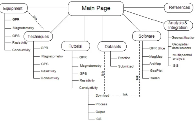
The Archaeogeophysics.org website will be composed of integrated yet separate sections, that are inter-linked and designed to address all aspects of geophysical data processing. From the main page, links are provided to seven different subheadings designating important components
for data processing: Equipment, Techniques, Datasets, Tutorial, Analysis and Integration, Software, and References. From these headings, it should be possible for a user to address specific aspects of geophysical data collection and/or processing. The following outline walks the reader through all components of the website as if they were accessing topics from the Main Page, which can be viewed online in its initial stages at archaeogeophysics.org. Figure 1 also illustrates the outline of archaeogeophysics.org and indicates some of the connections that will exist between the different headings:
Figure 1: Overview of Site Structure and Content Organization. Each primary branch represents an area of the site that will contain subsequent pages with detailed information and examples. Note: that the site is built to be dynamic through the use of a wiki infrastructure. Consequently, additional text, categories, photos, and instructions can be added by registered users as new kinds of training areas are required.
Main Page
1. Equipment: This section of the tutorial will contain information regarding the different types of geophysical equipment available for survey. It will include product information as well as descriptions of types of equipment. CSULB will provide information about the types of equipment available at our facility, and this section can be built upon by users’ experiences with other types/brands of equipment. Discussion on the following types of equipment that will be provided by CSULB are:
i. GSSI SIR-3000 Ground-Penetrating Radar b. Magnetometry
i. Geometrics G-858 Cesium Vapor Magnetometer ii. Geometrics G-856 Proton Magnetometer
c. Resistivity
i. OhmMapper TR 1 Capacitively Coupled Resistivity d. Conductivity
i. EM38B Conductivity Meter e. GPS
i. Trimble Pathfinder ProXR
2. Techniques: This section will contain the majority of the information regarding geophysical data processing. It will be configured similar to content provided in Wikipedia pages, in that it will contain paragraph-style information with links for more detailed instructions. In the techniques section, important steps in data processing for each piece of geophysical equipment will be discussed, with links to more detailed instructions contained within the tutorial section. The techniques section will discuss why specific steps are important so that the user understands how and why to process data so that it is understood beyond following step-by-step instructions. For example, components that will be discussed within the GPR section our outlined below:
a. GPR i. Download ii. Process iii. Filter iv. Output v. GIS integration b. Magnetometry c. Resistivity d. Conductivity e. Trimble GPS
3. Datasets: The datasets section will initially contain a “practice” set of data consisting of a geophysical survey conducted in the fall of 2007 of a burial plot located in Zzyzx, CA. This dataset contains GPR, Magnetometry and
conductivity data collected over the same 15x15m grid. Its size and multiple technique component make the CSULB Zzyzx data an excellent practice set from which the tutorial section will be built. Once the site is in use, the datasets section will also be a place where users can upload their own data in an effort to share geophysical analyses. Therefore, the datasets section will consist of the following components:
a. Practice dataset b. Submitted datasets
4. Tutorial: The tutorial component of the archaeogeophysics website will house the step-by-step instructions for data processing of GPR, magnetometry, conductivity, resistivity, and GPS units. These tutorials will contain written instructions, as well as photographs and videos highlighting important steps within the processing. Tutorials will be provided for the following instruments:
b. Magnetometry c. Resistivity d. Conductivity e. GPS
5. Analysis and Integration: This section of the wiki will focus on integrating geophysical data into GIS for further spatial analyses. This portion of the tutorial will include incorporating multiple geophysical techniques into one GIS file for interpolation, as well as applying various statistical analyses via ArcGIS. The analysis and integration component will contain but is not limited to the following aspects:
a. Georectification
b. Geospatial data sources c. Multispectral analysis d. GIS
6. Software: The software section will contain brief descriptions of available
software for geophysical data processing. This section will also have a large user component, as people can upload links and information for software not currently used in CSULB data processing. The software section will contain information and links for the following programs:
a. GPR Slice b. MagMap c. Radan d. GeoPlot e. ArcMap
7. References: The final component of the Main archaeogeophysics page will be a list of references for users who want more in-depth information regarding geophysical data processing. This section also contains a user component, as people could upload articles, books, and links for information they find useful. The following are descriptions of the content of each sub-heading from the main page of archaeogeophysics.org. This portion of the outline is intended to walk the reader through the various components of the wiki website, as if they were accessing them from the wiki site. Equipment
Introduction
Though the principles behind the geophysical instrumentation remain the same the models and configurations may vary which can present additional considerations in survey design. Presented below are some of the models that have been used to conduct geophysical surveys of archaeological materials. The models presented below are not meant to represent the full range of the available brands and configurations but merely a sampling of the
instrumentation in which the contributors of this wiki have familiarity with.
GPR
Description: A GPR system with interchangeable antenna and cart mounting and wheeled odometer capabilities.
Company: Geophysical Survey Systems Inc. Website: http://www.geophysical.com/ Abbreviated Specifications: 400 MHz Antenna Depth Range: 0-4m Weight: 5 kg Dimensions: 30 x 30 x 17 cm 900 MHz Antenna Depth Range: 0-1m Weight: 2.3 kg Dimensions: 8 x 18 x 33 Magnetometry
Geometric 858 Magmapper (Cesium Vapor Magnetometer/Gradiometer)
Description: An over the shoulder Magnetometer rig with a forward belt mounted computer unit. Company: Geometrics Inc.
Website: http://www.geometrics.com/858-d.html Abbreviated Specifications:
Operating Range: 17,000 nT to 100,000 nT Information Bandwidth: <0.004 nT / HzRMS Heading Error: < +/- 1 nT
Gradient Tolerance: > 500 nT per C’
Resistivity
OhmMapper Capacitively Coupled Resistivity System
Description: A waist belt mounted computer with a posterior drag antenna/receiver rig. Company: Geometrics
Website: http://www.geometrics.com/OhmMapper/ohmmap.html Abbreviated Specifications:
Operating Range: <3 to >100,000 ohm-meters Cycle Rate: up to 2 times per second
Conductivity
EM38B Conductivity Meter Company: Geonics Limited
Description: An over the shoulder conductivity unit with an unmounted exterior computer. Website: http://geonics.com/html/em38.html Abbreviated Specifications: Intercoil Spacing: 1 m Operating Frequency: 14.6 KHz Conductivity Range: 100, 1K mS/m In-Phase Range: +/- 29 ppt
Techniques
The appropriate geophysical techniques that should be employed in an archaeological investigation will vary from location to location. Each technique has strengths and constraints that make it more or less effective in detecting sub-surface features depending on the conditions of the environment associated with the archaeological investigation. The purpose of this section is to explain exactly what each technique measures, the strengths and weaknesses of each technique, and the conditions which allow the technique to be most useful.
Ideal Conditions for Geophysics
Level fields with short mowed grass are best suited for geophysical surveys because dense vegetation and other impediments can hinder efficient movement of the
instruments over the landscape. The speed of a geophysical survey is inversely related to the number of impediments that must be dealt with (buildings, trees, large rocks, bushes, gravestones, etc.), the nature of ground cover (open fields, short mowed grass, vs. tall grass or weeds, rocky terrain), or variability in the ground surface (level of slope). Steep slopes can make movement of heavy instruments difficult (e.g., large GPR antennas) and the use of some instruments is based on a uniform rate of movement in a given time interval or a uniform altitude above the ground, which is made difficult by steep slopes or vegetated areas. Ideal open ground for archeo-geophysical
surveys.
In this study area trees and gravestones are impediments to survey.
Owing to the size of most instruments it is frequently difficult to use them within heavily vegetated areas or move them between trees in forests. Moreover, because of the sampling schemes employed in area surveys to uniformly sample the ground (see traverses and samples), dense vegetation cover can make them impossible to employ if straight lines must be walked.
Some conditions only affect specific kinds of instruments. For example, rocky, very hard, or very dry ground makes electrical resistivity survey difficult or impossible to undertake because it may not be possible to insert probes in the ground or initiate current flow.
impediments to survey.
Good and poor conditions for conducting geophysical surveys at archaeological sites
Good Conditions • Level ground, open fields, short mowed grass, few impediments to movement (trees, rocks, buildings)
Poor Conditions
• Many impediments (trees, rocks, buildings, crops) • Heavy vegetation (bushes, tall grass)
• Forests • Wetlands
• Steep or variable slopes • Rocky terrain
• Large amounts of metallic litter or debris can preclude
use of magnetometers or EM instruments
• Overhead power lines can adversely affect instruments • Passing cars or cars in a parking lot can affect
magnetometers and EM if nearby
• Electrical storms can affect EM instruments from large
distances
GPR
Ground-Penetrating Radar produces large scale, high resolution structural information about subsurface deposits. GPR takes into account the effects of wave propagation by measuring the speed of an emitted electromagnetic wave and its travel time as an antenna is dragged across the ground. This allows depth of buried features to be calculated. GPR does not provide a
picture of what is beneath the ground. What is detected is time. Detection of features is seen as changes of the return of the signal.
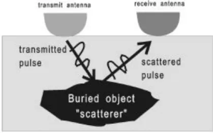
As the antenna is dragged across the ground, electromagnetic waves are radiated from the antenna and travel through the soil at a velocity determined mainly by the permittivity of the material. As it travels downward the wave spreads out until it hits an object that has different electrical properties from the surrounding medium. This wave scatters and portions rebound and are received by a receiving antenna.
Figure 1: The movement of electromagnetic waves as they encounter a buried object
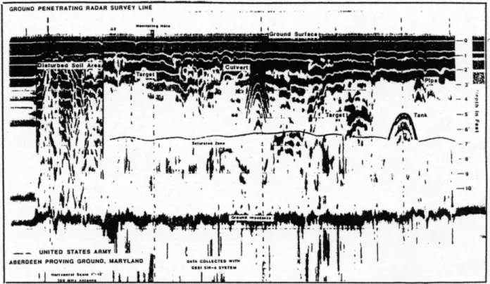
The distance from the wave source to a buried object is equal to the wave speed times the travel time. The intensity of the reflection of subsurface features is also interpolated and the greater the reflection coefficient the larger the signal appears in the radargram. The dialectric constant is an important component of Ground Penetrating Radar (GPR). It is a measure of how transparent an object is to the radar. Features in the subsurface are seen as changes in the radar signal as it returns to the machine. Objects buried in the ground create hyperbolic reflection patterns. For example, clay is impenetrable with GPR, so pits in clay layers can be very easily picked up.
Figure 2: Ground-Penetrating Radar survey depicting hyperbolas as the radar signal changes when objects are encountered.
Magnetometry
Magnetometry generates compositional information about the subsurface and near surface deposits. Magnetometry measures anomalies in the earth’s magnetic field. This
magnetic field is generated because the earth’s core consists of iron compounds in a dense liquid state. The revolution of the earth results in a magnetic field with circular lines of flux running from the North to the South Pole. The Global Magnetic Field refers to the pattern of flux caused by the earth’s massive structure, but a Local Magnetic Field also exists. This pattern of flux is the result of much more localized phenomena which can be archaeological in context. The degree of soil magnetization at any given point is a product of the global field strength and the local magnetic field of the soil, also referred to as the magnetic susceptibility of the soil. Localized magnetic features can enhance or dampen the field, creating anomalies on maps generated from magnetometry readings. Cultural features that may create magnetic anomalies include pieces of ferrous material, alignments of high-iron volcanic rocks, ceramics and bricks, ditches filled with organic-rich sediments, iron-containing soils, and sediments subject to intense heating.
Figure 3: Diagram of earth's magnetic field combining with the anomalous magnetic field of an archaeological object (from Weymouth 1986).
The ideal circumstances from magnetometry surveys include an area in which
background is uniform so that anomalies stand out upon correction for diurnal variation. The diurnal refers to the magnetic fluctuations which occur hourly due to the gravitational forces of the sun and moon. These variations are usually small and smooth, and range from only 50-100 gammas. The diurnal is a variable which must be accounted for in magnetometry, because since it is always present the diurnal variation must be accounted for so that the correct magnetic flow can be accounted for on a specific day at a specific time. It is only by doing this that changes in the earth magnetometry can be attributed to something physical beneath the soil and not as a result of variations in the earth’s own magnetic field.
Three different types of magnetometer machines exist. The Fluxgate magnetometer was introduced in 1961 and is still widely used, especially in England. It must be pointed north and provides reasonable fine scale discrimination and high resolution. The proton magnetometer has a sensor mounted on a staff which contains a coil immersed in a proton-rich liquid. When the magnetometer is being operated, a current passes through the coil for 2 seconds, then stops. The then charged protons become polarized in the artificial current and spin with the sensor, and as the current stops they align themselves with the local magnetic field. This is called precession, which is the combined effect of the gravitational attraction of the planet and the local magnetic susceptibility of the soil on spinning protons. The final machine available for magnetometry survey is a cesium vapor magnetometer. This technique measures variability in the earth’s magnetic field using a self-oscillating split-beam Cesium Vapor (non-radioactive Cs133) with
automatic hemisphere switching. Cesium vapor magnetometers exploit the changes in optical transparency of the cesium vapor when exposed to magnetic fields. A cesium vapor
magnetometer measures the frequencies of oscillations of cesium electrons. The G-858 is
actually a magnetic gradiometer because it has two magnetometers separated by a small distance. By subtracting the magnetic field measured by each magnetometer, external fields such as the Earth’s field are eliminated making weak near surface anomalies more apparent in the acquired data. The cesium vapor magnetometer is much more recent, and allows many more
measurements per second to be taken than the other two types of machines.
Figure 4: The Proton Magnetometer
Resistivity
This technique measures how strongly the soil opposes the flow of electric current. A low resistivity indicates soil that readily allows the movement of an electrical charge. Different materials have different resistance levels which are usually linked to the water content of the material. Therefore, it is often better to conduct resistance surveys when there is less moisture in the ground.
Resistance works under the principle of Ohm’s Law (R=V/I) and can be determined by monitoring the change in voltage (V) as the measured current (I) flows through a material. Resistance is usually expressed in Ohms (Ω). Remember that resistance is a bulk measurement and relates to how much of a material is present as the current flows through it. In archaeology the measure of resistivity (ρ, measured in ohm-m) is often better to use because the measurement created will not change with the size or shape of the material. The electrical resistance in soil varies and can be affected by the presence of archaeological features.
Hard, dense materials such as stone walls, mounds, banks, cobble, rubble, paving, rubble-filled pits, and stone coffins/tombs typically have high resistance. These structures usually allow
for good drainage or lack moisture. Low resistance occurs where areas retain moisture.
Ditches, soil-filled pits, hut circles, foundation trenches, graves, gullies and furrows, metal pipes all exhibit low resistance. Remember that archaeological structures are seen as changes from the background resistance.
Figure 7: Archaeological features such as ditches and pits often have greater levels of moisture thus be less resistive than the soil around them. Stone walls or foundations have smaller levels of moisture thus have a greater level of resistance than the soil around them. These differences in resistivity stand out compared to the soil around them.
The resistivity meter emits pulses of weak electrical current into the earth and a receiver on the instrument detects the level of resistance in the soil which is recorded on a data logger. Patterns of resistance are thus recorded and can then be plotted using programs such as Magmap. These patterns may then be interpreted and compared to other geophysical data.
Two types of resistivity machines are used in archaeology: Galvanic and capacitively coupled instruments. Galvanic resisitivity is older and requires direct contact in the form of probes inserted into the ground. The probes are connected to a DC power source and the measured voltage is used to calculate resistivity. Usually the techniques require 4 probes: 2 for measuring and 2 used to induce the current. Different arrays of the probes make anomalies look different. Capacitively coupled resistivity is similar to Galvanic, but contact is not made
directly, but capacitively at a frequency of 16kHz, and an antenna is used to transmit and record voltage as opposed to probes.
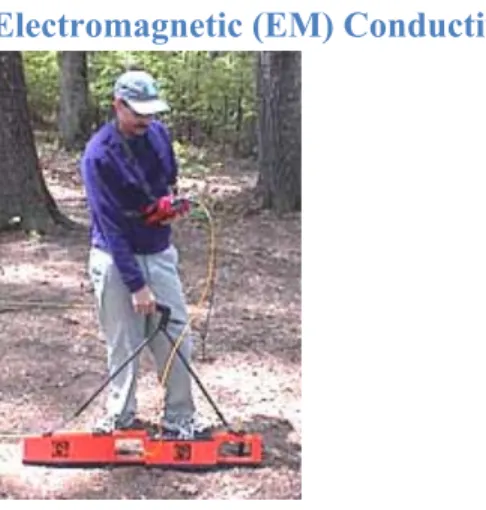
Electromagnetic (EM) Conductivity
Figure 8: The EM38B Conductivity Meter
This technique is basically the inverse of resistivity. It measures the ability of the soil to conduct electricity. EM conductivity produces an alternating current in a primary coil which induces the flow of eddy currents into the ground. These eddy currents generate a “secondary magnetic field” which produces current flow in a receiver coil located at the opposite end of the instrument from the primary coil.
Things which conduct electricity easily show up as highs in conductivity, which could be indicative of potential buried materials. EM conductivity is generally less sensitive than
resistance meters to the same phenomena. However, conductivity allows for much faster data acquisition and can be used in conditions unfavorable to resistance meters. Conductivity meters respond strongly to metal which may be a disadvantage when metal is extraneous to the
archaeological record. On the other hand it can be very useful when metal is of archaeological interest. Conductivity can record at depths between 4 and 6 meters depending on coil separation, and can be used vertically (good for finding features) or horizontally with no physical contact to the soil necessary. Archaeological materials easily detected through conductivity are similar to those detected through resistivity and include walls, foundations, roads, wells, canals, pits, hearths, and graves.
GPS
The Global Positioning system is a navigational system that utilizes the position of orbiting satellites in space to calculate the position of a global positioning receiver. Since the paths of satellites move around the earth in
relatively fixed orbits one may utilize the precise timing and the known position of these orbital bodies from their outgoing signals as a spatial reference to calculate a position of a terrestrial receiver. In practice the global positioning system consists of three segments: the control, the satellite, and the receiver.
The control segment is the ground-tracking infrastructure that regularly monitors and controls the orbital position of the satellites. Satellites may be taken out of the available pool of satellites for a period of time in order to reduce the overall amount of error that may occur in cases where the satellite path varies significantly from the projected path. Satellites may also be taken out of the pool or reinstated with a time offset in order to purposefully decrease the
accuracy of civilian model GPS units.
The satellite component of the global positioning system consists of a series of orbiting satellite vehicles that continuously send data towards earth. The satellite utilized in the global positioning system orbits the earth in six orbital planes spaces 60 degrees apart and completes the same orbit around earth roughly once every 24 hours. Each satellite is also orbiting the earth with an obliquity of 55 degrees relative to the equatorial plane.
The receiver component of the global positioning system communicates with and receives the signals sent by these satellites and calculates it position based off of the known position of the satellites at a given time. With four or more satellites fixes a receiver is able to reliably locate its position in three-dimensional space on earth.
In order to increase the reliability of a satellite fix the receiver communicates with the satellite in a pseudo random code. This code not only identifies a specific satellite but also amplifies the satellite signal by stacking the encoded signal of both the receiver and the satellite to elevate the signal above earth’s ambient radio background.
Archival data stored in tracking stations across the earth on the degree precision of the projected and observed satellite positions as well as the latent atmospheric conditions, geodetic surface variations, and visibility. These are then factored into to create a differential correction for the positional data stored in the receiver units to arrive at a more accurate reflection of the receiver’s actual position in time and space
Datasets
The datasets component of archaeogeophysics.org is the portion of the website in which real data will be placed. This section is important, because it will allow users to practice data processing with previously recorded geophysical data. The initial datasets section will contain geophysical data recorded from a project conducted by CSULB, with the hope that users will upload their own datasets in the future. The practice dataset will contain the raw data from a GPR, magnetometry, conductivity, and resistivity survey. This practice data will also be utilized in the tutorial section of the wiki, so that users may follow along the steps while practicing with the actual data.
Practice sets:
These pages will include downloadable data files collected at various locations that are accompanied by instructions on how to download and save raw data. Links to other pages that provide information on how to process the data will be imbedded in the text of these pages. Practice data sets such as the one from Zzyzx can provide a model for conducting archaeological survey using a top down approach method which examines a potentially culturally significant locations starting with large scale examining techniques such as remote sensing (e.g. satellite imagery, aerial photography) and moving on to collect data in a more concentrated area using surface survey and remote sensing. This methodology is efficient, cost effective, and eliminates costly guesswork associated with antiquated techniques of archaeological survey.
Practices with the datasets included the one from Zzyzx will allow users to become comfortable with the different software programs associated with processing raw data and interpreting it. The analysis of data collected in the field can contribute to determining a location’s eligibility for the National Register with very little impact to the integrity of the location’s archaeological record.
Zzyzx, California SBR-05417
Data collected from a geophysical survey at Zzyzx, CA in the fall of 2007 yielded GPR, magnetometry and conductivity data of a supposed burial plot. This data will be uploaded in its raw form, so that users may practice geophysical analysis on an actual dataset. Just South of Soda Springs (Zzyzx), California in the Mojave Desert is the site SBR-05417. The site is a large camp site on the west side of sand dunes. There are visible hearths in the blowouts and various surface artifacts including ground stones, projectile points, ceramic sherds, and fire cracked rock.
As the area of the site is quite expansive, large-scale excavations would be extremely expensive and time consuming. In order to obtain more information about the archaeological record at the site our class employed a top down approach to data acquisition at site SBR-05417. This approach first employs techniques that acquire data on a large scale with minimum cost and invasiveness then proceeds gradually with smaller scale data acquisition requiring graduated cost and invasiveness. In this instance, we first sought out existing data on the area through literature
research and satellite images from global databases. The next step was to employ a surface survey of the site to identify the locations of areas with high concentrations of surface artifacts. From this survey we choose an area that contained a relative high concentration of surface artifacts and laid out a 35m by 70m grid in which we performed surveys with various geophysical instruments to obtain information about the subsurface without expensive
excavation. We also launched a blimp with a camera rig in order to take aerial photographs of the terrain that we surveyed.
The data set that will be available on Archeogeophysics.org will include raw data collected with the GSSI SIR-3000 ground penetrating radar, the Geometrics 858 Cesium Vapor Magnetometer, Geometrics Ohmapper Capacitively Coupled Resistivity instrument, the EM38B conductivity meter , and the Tremble GPS Pathfinder. In addition to these raw data sets,
satellite images and aerial photographs will also be available to provide a back drop when compiling processed data into ArcGIS.
The Zzyzx dataset page will include various links to individual specific task based pages in the tutorial section that will instruct the user on various ways to integrate and analyze
processed data in Arc GIS. The following tutorial pages using the Zzyzx data will be available. • Importing geophysical data into ArcGIS
• Georectification of geophysical data
• Generating Topographic Maps in ArcGIS using data collected with GPS • Interpolation of raw geophysical data within ArcGIS
Submitted
This section will house other collections of geophysical data as users upload them, in an effort to increase accessibility of geophysical data as well as to provide users with alternate data for analysis.
Tutorial Page Introduction
This page will provide step-by-step instructions on how to operate geophysical
instruments in the field as well as how to process data recovered from the field. As the web site grows, we will introduce additional pages that cover instructional guides to integrating
geophysical data into Global Information Systems. GIS programs like ArcMap are dynamic tools in the compiling and analyzing geophysical data along with other data sets. Each page will generally focus on individual tasks, but each page will contain links to other instructional pages as well as general information pages that inform on concepts and techniques as described above. This document presents only a portion of the information that will be available on the web site. The information presented here will provide a basis for collecting and processing data, and will be among the first information available on Archeogeophysics.org.
Ground Penetrating Radar
One of the most promising of geophysical methods for rapid terrain characterization at depth is ground-penetrating radar (GPR). In this method an antenna is dragged over the surface of the ground producing nanosecond/time data in graphic form. These data may be converted into depth/x-y location as needed with relative ease. Such an instrument may be towed at rates of up to 10 miles an hour, making GPR an immediately practical large area tool.
1. Our GPR equipment consists of GSSI’s SIR-3000 with a 400 or 900 Mhz antenna. This relatively compact unit is entirely self-contained and is capable of generating immense amounts of data across wide areas.
2. The GPR unit can be configured on a 3-wheeled cart or using a harness and hand held device.
3. Locational information is provide via markers that are set by the user (like the magnetometer), a survey wheel which measures out distance (the cart is built with a survey wheel), or a GPS unit (the Ag132 and 214 can provide locational information for the GPR.
4. The GPR is powered by 1 Lithium Ion Laptop battery. This battery lasts about 3 hours when fully charged. We currently have 2 such batteries.
5. Good ground coupling between the antenna and ground is required for the GPR. It is essential that the antenna make good contact with the ground at all times. As a result, a survey must often be prepared prior to surveying and an individual should proceed the survey to clear away rocks, etc. In very rough terrain the cart will not work and the handheld harness must be used.
6. The amount of memory in the SIR-3000 unit is 1 gigabytes which is adequate for large survey areas. Data can be moved to a computer via a flash card or a USB connection directly to a laptop.
7. Settings for the SIR-3000 are numerous but we usually use these: 8. 512 scans/sample
9. 60 ns measure time
10. 8-bit data (GPR-SLICE only requires 8-bit rather than 16-bit data)
information. This is done using a tape and the SIR-3000 software.
12. Transects get made in the same way as the resistivity survey – in back and forth
fashion. Be sure to record, however, the direction that the transects take: starting point, initial direction, transect interval.
13. The SIR-3000 records each transect as a separate ‘profile.’ Profiles are stored as individual formats using a sequential numbering system. E.g., FILE___001.dzt,
FILE____002.dzt, etc. Thus is important to keep track of the layout of the survey and the location of each transect. This information must be kept in a field notebook. 14. Refer to the SIR-3000 manual for specific operating instructions. .
Quick Start for Sir3000 Setup with 400 MHz antenna
A. What you should see in the menus:
1. Insert battery after cabling has been connected and you are ready to collect data 2. After the TerraSIRch main screen comes up, press the TerraSIRch tab (bottom left
Function Key)
3. Right arrow on Collect directory 4. Down arrow to Radar
5. Right arrow on Radar and make sure you see: a. 400MHz or 900 Mhz
b. T_Rate 100KHz c. Mode=Time d. GPR-None
6. Down arrow to Scan, then right arrow a. Samples=512 b. Format=16 bit c. Range=60 d. Diel=18* e. Rate=32 f. Scn/unit=32 (400Mhz) 64 (900 Mhz) 7. Down arrow to Position, then right arrow
a. Toggle to Manual, then to Auto, then back to Manual to re-servo b. Offset= whatever Auto sets c. Surface (%)=0.00
8. Down arrow to Gain, then right arrow a. Toggle to Manual to re-servo b. Set Gain Points =5
c. Toggle to Auto d. Toggle to Manual
e. GP1=you set if Auto not good f. GP2=you set if Auto not good g. GP3=you set if Auto not good h. GP4=you set if Auto not good i. GP5=you set if Auto not good
Acceptable Scan
9. Down arrow to Filters, then right arrow. You will need to set these differently for different antennas. For the 400 Mhz antenna, set the Filters to:
a. LP_IIR=800 b. HP_IIR=100 c. LP_FIR=0 d. HP_FIR=0
e. Stacking=3 (could change to 0-2) f. Bgr_Rmvl=0
For the 900 Mhz Antenna, set the Filters to: g. LP_IIR=2500
h. HP_IIR=225 i. LP_FIR=0 j. HP_FIR=0
k. Stacking=3 (could change to 0-2) l. Bgr_Rmvl=0
*see Appendix D, p. 59, in manual. This is not a critical setting.
**This setting is for distance data collection using survey wheel only B. What do you do if the above settings do not appear?
Recall Setup if you saved the Setup:
1. Down arrow to System, then right arrow 2. Down arrow to Setup, then right arrow
3. Down arrow to Recall, the press center button
4. Up arrow to Setup01 or where you saved it, press right arrow
5. Now recheck all your settings under A (above) and adjust as necessary. C. How to Save your Setup
1. Down arrow to System, then right arrow 2. Down arrow to Setup, then right arrow
3. Down arrow to Save, select any one Setup from Setup01 to Setup 16. 4. Press right arrow
D. What to do if you did not save Setup: 1. Down arrow to System, the right arrow 2. Down arrow to Setup, then right arrow
3. Down arrow to Recall, then right arrow, scroll to 400met, then right arrow 4. Recheck all settings under A above.
E. How to Download files from Sir3000 to USB memory stick
1. Boot Sir3000 to TerraSirch by removing and reinstalling battery. 2. Insert USB key into its slot on Sir3000 after the main menu comes up
3. Press the TerraSIRch tab (bottom left Function Key) 4. Press Run/Stop
6. A window appears with all your files. Use center arrow to select your files 7. Press right arrow to begin file transfer
8. Remove memory stick and insert into your computer F. Important tips:
1. After you change a setting, give the control unit time to execute its function or you may lose your setting.
2 Position is time zero, the beginning of the scan. Toggle to Manual, then to Auto, then back to Manual and set Surface to zero.
3. Apply Gain if needed after you have set Surface to zero. Toggle to manual, then to Auto, then back to Manual and set gains as needed.
4. Field note format (following pages)
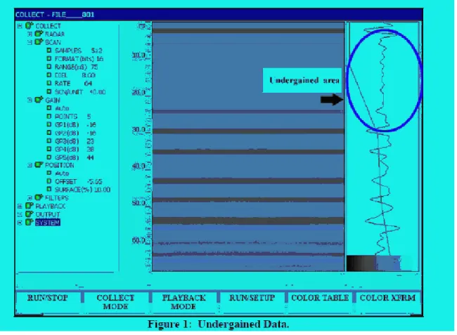
Simple Fix for Undergained Data-
Overview: The use of 5 gain points with certain time ranges can sometimes lead to the direct wave being position between gain points 1 and 2. Since the direct wave is often the highest amplitude wavelet in the trace, the SIR-3000’s auto gain servos will depress the adjacent gain points (1 and 2) in order to prevent signal saturation (clipping). This can result in the top 20% or so of the time range to appear undergained (Figure 1).
Figure 1: Undergained Data.
The Fix: In order to correct for this, you will need to manually adjust the Offset. 1. Under COLLECT>POSITION, toggle the Auto servo to Manual.
Highlight OFFSET and click enter to bring up the offset value dialog. You will see the full trace. Click the UP arrow and you will see a black, horizontal line on the data. Reposition this line close to the first positive (right hand side) rise of the direct wave. You should get an offset number near 0 (Figure 2). Click the Right arrow to make the change.
2. Next go to POSITION>SURFACE(%) and change the surface % to 0.00.
3. Toggle the Auto gain servo to Manual and then back to Auto and you will see a better normalized trace (Figure 3).
4. Save these settings under SYSTEM>SETUP>SAVE.
Magnetometry
This next section includes information that will be available on the magnetometry tutorial page. The page will provide steps for setting up and using the Geometrics 858 Cesium Vapor Magnetometer. This is the particular instrument used by the by the faculty and students of CSULB’s archaeology program. There will also be a flow chart that can guide a person through the steps of processing the data retrieved from the field. Additional and more detailed steps to working with the processing software MagMap will be provided in the software section of the website.
Magnetometrv Procedures
A magnetometer is an instrument for measuring the intensity of the earth's magnetic field. Most rocks contain magnetite, the most common magnetic material, and therefore produce some disturbances in the magnetic field. Soils and even some manmade objects such as pottery can have magnetic properties. Through interpretation of magnetic readings, assumptions can be made about what exists below the surface, whether it is a pipeline, an ancient hearth, or a geologic structure.
Diagram of earth's magnetic field combining with the anomalous magnetic field of an archaeological object (from Weymouth 1986).
Geometrics 856 Base Station
A. Familiarize yourself with operation manual for the instrument. We will be using GeoMetrics Model G-856A. Be certain the instrument has batteries; the correct decane level; correct date, time and switch (#1-4 = OFF) settings. You should also make certain the device is appropriate tuned.
B. The 856 is used as a base station. This means that it is left unattended and stationary during the period of the magnetometer survey. Readings are made on
the base station every 15-seconds. These readings are used to correct the local magnetometer readings for macro and micro pulsations caused by diurnal changes and magnetic storms.
C. All data are stored internally by the 856 to allow for automatic, unattended operation.
D. Setting up the base station.
a. Find a location that is at least 100 meters from any activity, large metal objects and where it is unlikely to be disturbed. Remove all iron from the area to be surveyed (use metal detector if need be). Check immediate vicinity for iron, fences, power lines, etc. that may influence readings.
b. Use spoon coring device to create a hole that is at least a foot deep to hold the sensor rod.
c. Connect the aluminum pole together and mount the sensor to the 10 foot staff.. Mount the sensor in the VERTICAL position (so that the long axis is perpendicular to the ground.
d. Attach sensor cable to gray rectangular main control box.
e. Place the aluminum pole into the hole and brace with material so that pole and sensor are securely situated.
f. Make certain that the sensor is orient to the NORTH. There is an arrow on the top of the sensor that indicates which direction should point north.
g. Check the tuning and retune if necessary to get maximum signal strength, and record.
h. Check battery levels.
E. Perform an instrument check, i.e., take several successive readings in one location without moving and note the repeatability; and record the results.
F. Check battery conditions.
G. Erase all old data by pressing the following sequence of keys: RECALL - SHIFT - 0 - ENTER - ERASE - ERASE.
H. Be certain the top sensor arrow is pointed north during all readings. I. Record the location of the base station.
J. Synchronize the clock with the Geometrics 858 unit. i. The units should be synced to the nearest second.
ii. You will need to know the Julian Day – which is the day of the year in order to set the date/time.
iii. Press: AUTO TIME SHIFT (day) + (day) + (day) + (hour) + (hour) + (minute) + (minute) + ENTER
K. Initiate automatic recording of data by hitting the following sequence of keys: AUTO SHIFT (seconds) + (seconds) ENTER
L. Once you have started the automatic recording make certain no one approaches the base station.
M. When you are finished press: AUTO CLEAR to stop the machine.
N. Data will be downloaded via MagMap 2000 software into the computer at the end of each day after use. Refer to the MagMap 2000 manual for downloading instructions.
Geometrics 858 Cesium Vapor Magnetometer
A. The Geometrics 858 magnetometer is an instrument that measures variability in the earth’s magnetic field using a self-oscillating split-beam Cesium Vapor (non-radioactive Cs133) with automatic hemisphere switching.
B. Familiarize yourself with operation manual for the instrument.
C. PRIOR to setting up instrument, lay out a blue tarp
to put all cases on. Make sure you put the instrument together OVER the tarp so that any parts that fall off (cables, bolts, etc.) fall onto the tarp and not into the grass.
D. Put the instrument together following the instructions in the 858 manual.
E. Be CAREFUL with all cables and connections. The most fragile parts of the equipment are the connections.
F. Be very careful with the sensors - -these are delicate and expensive. Do NOT drop them or treat them poorly or you will be sold.
G. Be certain the batteries are well charged, the data collector has the correct date and time settings.
H. Make certain you are wearing no metal objects – no eyeglasses, belts, shoe eyelets, etc. I. Survey Set Up
a. Decide beforehand the area you wish to survey. Plan a series of grids of at least 50x50 meters in size. The use of grid units (even with GPS) makes it easy to stop and restart work and to append new data from multiple days.
b. Lay out the survey transect with nonmagnetic tapes and stakes. Remove all iron from the area to be surveyed (use metal detector if need be).
c. Check immediate vicinity for iron, fences, power lines, etc. that may influence survey. Remove as much metal and electronic equipment from your person as possible. When near highways, take no readings while vehicles are present. d. Mount the sensors to the aluminum staff. Attach sensor cables to data collector e. Place strap over the same shoulder that you will hold the magnetometer rod. J. Perform an instrument check, i.e., take several successive readings in one location
without moving and note the repeatability; and record the results. Periodically check battery conditions throughout the survey.
K. Be certain the sensors is pointed in the same direction during all readings and that the operator is in the same relation to the sensors at all readings.
L. Keep the sensor approximately 10-cm from the ground surface. Keep a CONSTANT height from the surface.
M. Record the transects by number consecutively within site/tract, give interval, and number stations on the transect consecutively or by tape distance from one end or the other and record. If you are not using a GPS unit, you must be certain that both termini of the transect are recorded in the referential system.
N. Reading are automatically collected 10 times a second once you hit the green START button.
O. Locational information:
a. If you are not using a GPS unit, you must mark your progress at a regular interval (e.g., 1 meter). Use a marked rope as a guide line for when to hit the
MARK button on the data recorder. Find a regular, even pace to record the data. b. If you are using a GPS unit, locational information will be collected for at a rate indicated by the output of the GPS unit. Typically that is 2-readings a second. If the GPS is working, you will see an indicator on the 858 display screen for the RS-232 port input.
P. Listen to the tones of the 858. A constant high pitched tone indicates an error or a sudden out-of-bounds reading. This might mean that readings are not being collected correctly.
Q. Record whether the survey was conducted in a uni-directional or bi-directional fashion. survey segment.
a. If you survey in a bi-directional fashion, you must use the mag. cart and switch from pushing to pulling. This keeps the orientation of the sensors the same for each direction.
R. If you use the GPS to record the location, use the lightbar to indicate the quality of the GPS position information. Loss of satellite contact can degrade the signal from 1-cm to sub-meter to multiple meters. If you are not able to get at least sub-meter resolution, you should not try to use the GPS to provide locational information as the positions will be too widely variable to be of any use. In this case, go back to using marked ropes. S. Data will be downloaded via MagMap 2000 software into the computer at the end of
Resistivity
This sections section contains some of the basic information that will be available on the website regarding resistivity surveys, operation of instruments and processing data. Information regarding detailed software instruction will again be available in the software section of the website.
1. Resistance (measured in Ohms) is a function of the composition of the underlying sediment (particularly water content), the distance between the probes (the array) and the cross section of the current placed between the probes (typically 1 mA). If the distances between the probes, current are kept constant, then differences in resistance can be used to distinguish variable composition of the substrate.
2. All archaeological structures are seen as a change in the background resistance. The magnitude of the background resistance depends on the type of probe array use. It is useful to look at background resistance and the way it arises because this can act as an indicator as to the likely contrast that will be seen between archaeological structure and the surrounding medium. Factors such as soil type, topsoil thickness, underlying geology, drainage and climate all combine in a complex way to determine the background resistance.
3. Stone structures such as walls and roads are generally poor electrical conductors compared to the surrounding soil and so show an increase in background resistance. Soil filled ditches and pits generally tend to collect water that makes them better electrical conductors than the surrounding soil or rock and so show as a lowering in the background resistance. The figure below shows the typical resistance profiles as walls and ditches are traversed.
4. The Geometrics OhmMapper is a capacitively coupled resistivity meter that measures the electrical properties of rocks and soil without cumbersome ground stakes used in traditional resistivity surveys. A simple coaxial-cable array with transmitter and receiver sections is pulled along the ground either by a single person or attached to an all-terrain vehicle. Data collection is many times faster than systems using conventional DC resistivity. The
instrument has a number of key features that make it a superior instrument over traditional probe designs:
a. Measurements are made twice a second. As a result, a full dipole-dipole resistivity profile can be done in a fraction of the time taken for traditional resistivity
measurement.
b. Operates over frozen ground, ice, concrete, and other areas where grounded dipole measurements are difficult to make.
5. The setup of the OhmMapper is shown in the following diagram:
This section deals specifically with the Geometrics Ohmapper Capacitively Coupled Resistivity instrument . It also assumes that data will be processed by MagMap 2000 software.
A. Care of instrument. The instrument is rugged and more or less waterproof, so the only concerns are electronic:
a. Avoid pulling on any wires and/or connectors.
b. Use only the provided charger for the NiCd batteries, 10 hr maximum charge, or for partial discharge, charge number of hours used.
c. Keep antennas clean after use. d. Do not over tighten connections.
e. Be very careful with the connections to the computer.
B. Safety. While a shock is not likely; do not touch both antennas at the same time unless the instrument is turned off.
C. Instrument settings. Default settings are usually okay and changes are situational. D. Data generation.
1. Assemble the OhmMapper as instructed in this chapter. 2. Attach the OhmMapper G-858 console to the battery belt.
3. Make sure the clamp on the console cable is securely attached to the triangle tow loop as pictured in this chapter.
4. Attach a rope between the transmitter and receiver dipoles 5. Turn on the transmitter and receiver.
6. Snap the battery belt around your waist. 7. Turn on the OhmMapper G-858 console
8. Select OhmMapper Geometry from the main menu, hit enter, and enter the array geometry, and hit the escape key to return to the main menu.
9. Go to System Setup , select OhmMapper Test, and press enter. If the transmitter light is flashing, and the receiver light is flashing, and everything is connected properly you should see a string of readings displayed on the screen. See Chapter 9: System Setup for a description of what these readings mean.
10. Select a survey type. In general a Mapped Survey is the recommended survey type for an OhmMapper survey, although under certain conditions a Simple Survey is easier to configure. .
11. Set up the survey in the G-858 console for Mapped Survey.
12. Do a walk-away test as described in the FAQ section below to determine the maximum transmitter/receiver separation that can be used.
13. For an initial test it is recommended that traverses be done in both directions with the same rope length. For example if a profile is to be done on a 100 meter line with separations (rope lengths) of 2.5 meters, 5 meters, 7.5 meters, and 10 meters, the operator should walk the length of the profile up and down with the 2.5 meter rope, then up and down with the 5 meter rope, etc. until a total of 8 traverses have been made. This will allow a quality-control comparison of the data taken over the same line with the same Tx/Rx separation in two different directions. E. General concerns.
a. Lay out lines parallel to field structure, use very long transects at least 100 meters in length but 50 m. wide (10, 30 M also possible).
b. Survey should begin in the SW corner. Zig-zag pattern is time-saving and suitable except where low amplitude anomalies are expected.
c. Memory in the data collector is large enough to at least 4 50 grids on 1 M centers.
6. Antenna Spacing and Rope Length
A. Choice of antenna spacing is determined by depth to be surveyed; interval between readings and transects is determined by field structure and spatial resolution required.
B. There is a non-linear relationship between the spacing between the antennas (dipoles), the distance between the dipoles (rope length) and the depth measured. You can treat the OhmMapper as you would any standard resistivity meter. It uses
the same inversion software as a galvanic dipole-dipole instrument. The relationship between depth and n-factor is not linear with separation (n factor).
a. The n factor of a dipole-dipole resistivity array is the ratio of the distance between the receiver and transmitter dipoles to the length of the dipole. In terms of the OhmMapper this corresponds to the ratio of rope length to the transmitter and receiver dipoles lengths. For example if you are using 2.5 m cables the dipole length is 5 meters. If the rope separating the transmitter from the receiver is 10 m you have an array of n = 2. If the rope length is 20 meters then n = 4. If the rope is only 2.5 meters then n = 0.5.
b. In order to figure this out, you must calculate n-space for whatever configuration you have.
i. n-space = distance between dipoles (i.e., rope length)/ dipole length /
Dipole (m) Rope (m) n-space
2 2 1 2 4 2 2 1 0.5 5 2.5 0.5 5 5 1 5 10 2
c. You can then use this value to calculate the depth that you are measuring given any n-space. z / a
d. The median depth of investigation (Ze) for the different arrays. a is the length of the dipole. L is the total length of the array.
Ze/a Ze/L n = 1 0.416 0.139 n = 2 0.697 0.174 n=2.5 0.8295
n = 4 1.220 0.203 n = 5 1.476 0.211 n = 6 1.730 0.216
e. Thus, if one is using a dipole 5 meters and a rope length of 5 (n-space = 1), then median dept of investigation will be Ze = a* n = 5 * .416 = 2.08m.
i. If one is using a dipole of 2 meters and a rope length of 2 meters (n-space = 1) then median dept of investigation is Ze = a *n = 2 * .416 = 0.832m.
ii. If one is using a 2 meter dipole and a rope length of 5 meters (n-space = 5/2=2.5) then median depth of investigation. .8295 = Ze /2 Ze = 2* .8295 = 1.66 m.
iii. If we use a 5 meter dipole and a 2 meter rope (n-space = 2/5=0.4). This means that 0.2 = Ze * 2 = ca 1 meter.
f. Note that commercial inversion programs require n factors that are an even fractional integer such as 1 n, 2 n, ½ n, ¼ n, etc. Many can only use integer n factors such as 1, 2, 3, 4, etc. Fortunately RES2DINV can handle fractional n factors.
g. The OhmMapper samples are time based and positioned in space according to either GPS readings or mark positions. You can have different data distribution between two different marks if you walk at a different rate. The inversion software, such as RES2DINV, must have an even data distribution along the whole line. In order to do this we average the data to even distribution of data points along the entire line. In order to get this even distribution MagMap2000 averages the data to a unit called “Smallest Unit Electrode Spacing”.
i. If the smallest unit electrode spacing is 2.5 meters the data is averaged to one data point every 2.5 meters. The largest average you can use is determined by the largest common denominator or the dipole lengths and dipole separations you use. For example if you use 5m dipoles and 5, 10, 15, 20 meter separations the largest common denominator is 5m.
ii. But if you use 5, 10, 12.3, 15.1, and 20 the largest common denominator is 0.1 so the data must be averaged to those 0.1 meter, meaning you are forced to have a data point every 10 cm. This will give you a huge data set that the software may have difficulty handling.. Normal practice is to use a separation that is an binary fraction of the dipole length such as 5, 7.5, 10, 12.5, 15 meter separations (with 5m dipoles n = 1, 1.5, 2, 2.5, 3) which would give a maximum “smallest unit electrode spacing of 2.5m”. C. In the plowed field, antennas should be moved parallel to rows (i.e., not normal to the
D. When field furrows are pronounced, they may dominate the resistivity data.
Consequently, use the row width interval on a harmonic for the x-spacing and be certain to note these decisions in the log.
B. What Mark Spacing should I use?
a. You can use any mark spacing you like. It is only an external reference point to allow the software to correctly position the data. If you have chosen “Continuous” when setting up the survey mode the data sampling is time based at whatever cycle time you have selected. The default is 0.5 seconds, meaning you are
recording at a rate of 2 measurements per second. For example, if you have a flag in the ground every 10 meters then you set the mark spacing at 10 meters, and hit the mark button when you pass the flag. The software will correctly position the data at even intervals between the marks. On a Mapped Survey you tell the logger, when you set up the survey, what your mark spacing is. On a Simple Survey you have to remember your mark spacing and tell the MagMap software what you used.
C. Line Spacing
a. If you are only doing multiple passes over the same profile (same x-position) then it doesn’t matter what line spacing you use. This is only important if you are doing multiple parallel lines or 3-D surveys where you have multiple lines with multiple passes over each. A good rule of thumb is that in order to detect 3D affects the lines should not be more than one dipole length (n-space) apart. That is, if you are using a 5-meter dipole then the line spacing should be 5-meters or less in order to detect interline affects.
D. Data will be downloaded via MagMap 2000 software into the computer at the end of each day after use. Refer to the MagMap 2000 manual for downloading instructions.
E. Flashing Indicator Codes: a. Long = 1, short = 0
b. Voltage Code Current (mA)
000 16 001 8 011 4 010 2 110 1 100 .5 111 .25
Conductivity
Setup and Calibration of EM38B:
1. Q/P is the Quad Phase measurement or the conductivity reading for the sediment. The I/P is the In Phase measurement or the magnetic susceptibility reading. Each phase has a calibration knob on the console of the conductivity meter. These will be used to calibrate the unit prior to survey. The unit should be tuned multiple times throughout the day, especially as the temperature changes to keep the unit calibrated. As the temperature rises in the afternoon, it is particularly important to keep the unit calibrated as it will overheat and can potentially “lose its connection” causing data collection to cease until it has sufficiently cooled off enough to recalibrate. To calibrate:
2. Place EM38B unit on ground in vertical mode (console is visible from overhead view.) Make sure all metal objects (jewelry, the data logger, etc.) are as far away from the conductivity meter as possible. The unit is very sensitive to metal and any amount of metal objects nearby will alter the calibration.
3. Turn Power knob to Battery. The Q/P meter should read around 900 or above for a good battery. Change battery immediately if it reads between 400-600.
4. Turn Power knob to On.
5. Turn Q/P knob at end of EM38B console until Quad Phase meter reads zero. You may have to adjust the Coarse Control knob on the I/P console in order to zero the Q/P. 6. Once the Q/P is zeroed, use the fine and coarse control knobs on the I/P console to zero
the In Phase.
7. Lift EM38B unit 1.5m (roughly 5 feet) in the air and rotate it to horizontal mode so console is facing you.
8. Reset Q/P and I/P to zero following steps 4 and 5.
9. While unit is still in horizontal mode 1.5m in the air, set Q/P to an arbitrary number (e.g., 10.) Keeping instrument at same height, rotate unit to vertical mode and note the new reading of the Q/P (e.g., 16.)
10. Subtract the arbitrary number you chose from the new reading (e.g., 16- 10= 6.) Rotate unit back to horizontal mode and set the Q/P to the result of the equation (e.g., 6.) Rotate the unit back to vertical mode. If the unit is calibrated correctly, the Q/P will read twice the result of the equation (e.g., 12) while in vertical mode.
11. Check that the connecting cable is connected properly and securely between the data logger and the conductivity unit. You are now reading to set up the data logger to store data readings.
Setting Up Data Logger:
1. Turn on data logger (AllegroCE) and double click on the PocketDOS icon. A DOS command prompt screen appears (C:\>). Type in the command below and follow the instructions to begin data collection: