Efficient Training of Small Kernel Convolutional Neural Networks using Fast Fourier Transform

Wright State University Wright State University

CORE Scholar

CORE Scholar

Browse all Theses and Dissertations Theses and Dissertations 2015

Efficient Training of Small Kernel Convolutional Neural Networks

Efficient Training of Small Kernel Convolutional Neural Networks

using Fast Fourier Transform

using Fast Fourier Transform

Wright State University

Follow this and additional works at: https://corescholar.libraries.wright.edu/etd_all

Part of the Computer Sciences Commons

Repository Citation Repository Citation

Highlander, Tyler, "Efficient Training of Small Kernel Convolutional Neural Networks using Fast Fourier Transform" (2015). Browse all Theses and Dissertations. 1398.

https://corescholar.libraries.wright.edu/etd_all/1398

This Thesis is brought to you for free and open access by the Theses and Dissertations at CORE Scholar. It has been accepted for inclusion in Browse all Theses and Dissertations by an authorized administrator of CORE Scholar. For more information, please contact [email protected].

Efficient Training of Small Kernel Convolutional

Neural Networks using Fast Fourier Transform

A thesis submitted in partial fulfillment

of the requirements for the degree of

Master of Science

by

Tyler Clayton Highlander

B.S.C.S., Wright State University, 2014

2015

Wright State University GRADUATE SCHOOL

April 28, 2015 I HEREBY RECOMMEND THAT THE THESIS PREPARED UNDER MY SUPER-VISION BY Tyler Clayton Highlander ENTITLED Efficient Training of Small Kernel Convolutional Neural Networks using Fast Fourier Transform BE ACCEPTED IN PAR-TIAL FULFILLMENT OF THE REQUIREMENTS FOR THE DEGREE OF Master of Science.

Mateen Rizki, Ph.D. Thesis Director

Mateen Rizki, Ph.D. Chair, Department of Computer Science and Engineering Committee on Final Examination Matten Rizki, Ph.D. John Gallagher, Ph.D. Michael Raymer, Ph.D. Andres Rodriguez, Ph.D.

Robert E.W. Fyffe, Ph.D. Vice President for Research and Dean of the Graduate School

ABSTRACT

Highlander, Tyler. M.S., Department of Computer Science and Engineering, Wright State Univer-sity, 2015. Efficient Training of Small Kernel Convolutional Neural Networks using Fast Fourier Transform.

Convolutional neural networks (CNNs) are currently state-of-the-art for various

classi-fication tasks, but are computationally expensive. Propagating through the convolutional

layers is very slow, as each kernel in each layer must sequentially calculate many inner

products for a single forward and backward propagation which equates to O(N2_n2_{) per}

kernel per layer where the inputs areN ×N arrays and the kernels aren×narrays. Con-volution can be efficiently performed as a Hadamard product in the frequency domain. The

bottleneck is the transformation which has a cost of O(N2log₂N)using the fast Fourier transform (FFT). However, the increase in efficiency is less significant when N n as is the case in CNNs. We mitigate this by using the “overlap-and-add” technique reducing

the computational complexity toO(N2_log

2n)per kernel. This method increases the

algo-rithm’s efficiency in both the forward and backward propagation, significantly reducing the

training and testing time for CNNs. Our empirical results show our method reduces

Contents

2.2 Convolutional Neural Networks . . . 7

2.3 Convolution in the Frequency Domain . . . 12

2.4 Using FFT with Convolutional Neural Networks . . . 14

2.5 Overlap-and-Add . . . 15 3 Methods 18 3.1 Problem Domain . . . 18 3.2 System Design . . . 19 3.2.1 Image Pre-processing . . . 20 3.2.2 spaceConv Method . . . 21 3.2.3 FFTconv Method . . . 22 3.2.4 OaAconv Method . . . 25

3.2.5 Fully Connected Layer . . . 26

3.2.6 Softmax Layer . . . 28

3.3 System Complexity . . . 28

4 Analysis 31 4.1 Training Consistency . . . 31

4.2 Time vs. Number of Kernels and Input Depth . . . 32

4.3 Time vs. Kernel size . . . 33

4.4 Time vs. Input Size . . . 35

5 Conclusion 39

List of Figures

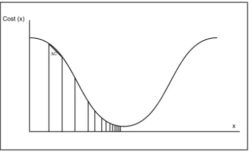
2.1 Gradient Descent Illustration . . . 6

2.2 Standard Convolutional Neural Network . . . 7

2.3 Convolution Illustration . . . 8

2.4 Sub-sampling Illustration . . . 8

2.5 Convolutional Neural Network for ImageNet 2012 . . . 11

2.6 Fast Fourier Transform Implementation . . . 14

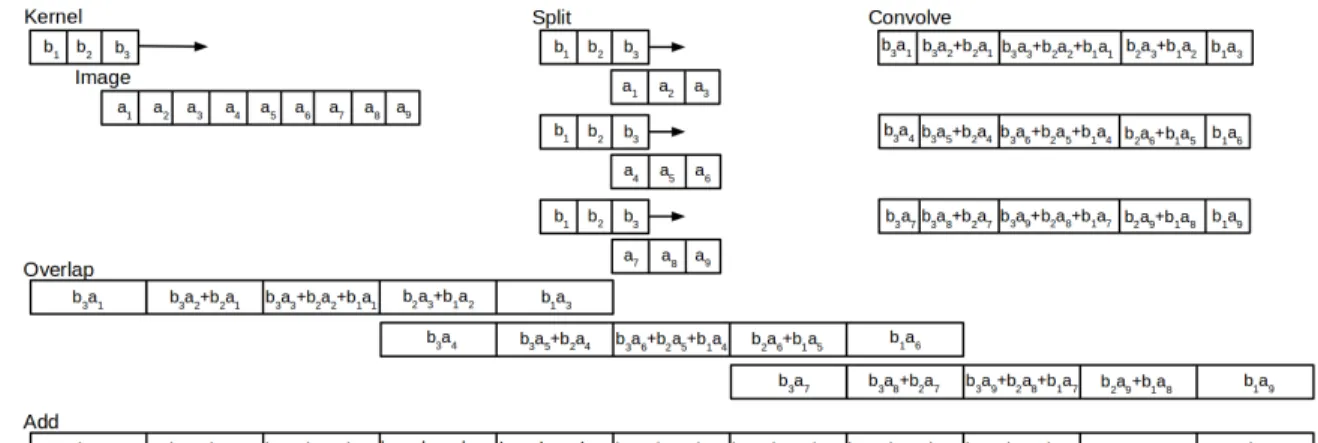
2.7 1-D Overlap-and-Add convolutions. The kernel is convolved with the im-age. The image is split into subset that are equal in size to the kernel. Each subset is convolved with the kernel. The subset convolutions are over-lapped then added together to produce the equivalent convolution. This example is done in the spatial domain, but the concept transfers to the fre-quency domain. . . 17

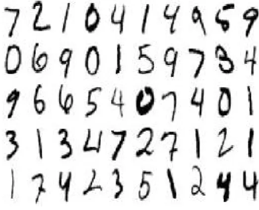
3.1 MNIST Digits . . . 19

3.2 The CNN . . . 20

3.3 FFT Benchmarks . . . 21

3.4 Single MNIST Digit . . . 21

3.5 Specific Form of the Convolutions . . . 23

3.6 FFTconv Forward Propagation . . . 23

3.7 FFTconv Weight Change Propagation . . . 24

3.8 FFTconv Error Propagation . . . 25

3.9 OaAconv Forward Propagation . . . 26

3.10 OaAconv Weight Change Propagation . . . 27

3.11 OaAconv Error Propagation . . . 27

4.1 Time vs. Number of Kernels Forward . . . 33

4.2 Time vs. Number of Kernels Backward . . . 34

4.3 Time vs. Kernel Size Forward . . . 35

4.4 Time vs. Kernel Size Backward . . . 36

4.5 Time vs. Image Size Forward . . . 37

List of Tables

2.1 ImageNet 2012 Convolutional Neural Network Results . . . 11 2.2 DropConnect for MNIST Results . . . 11 2.3 Results of Mathieu’s Fast Fourier Transform Convolutional Neural

Net-work in 2013 . . . 15 2.4 Computational Complexity Comparison. spaceConv refers to the

tradi-tional convolution in the space domain, FFTconv refers to convolution via a Hadamard product in the frequency domain without overlap-and-add, and OaAconv is the method we implement in our CNN design. . . 15

4.1 100 Epoch Training Results for each Layer Type. The values represent classification accuracy on MNIST for each convolution method. All three methods generate similar results. . . 31 4.2 100 Epoch Non-stochastic Training Results for each Layer Type. The

values represent classification accuracy on MNIST for each convolution method. All three methods generate the same exact results . . . 32

Acknowledgment

I would like to take this opportunity to extend my thanks to my advisor Dr. Andres

Ro-driguez and Professor Mateen Rizki for the years of mentorship and wisdom, without them

I would be but a mere mortal.

I would also like to express my great thanks to Dr. James Lawton for providing the main

funding for this work through the Air Force Office of Scientific Research (AFOSR) and

Dedicated to

1 Introduction

1.1

Motivation

The proliferation in the use of sensor systems for monitoring and surveillance has led to an

exponential growth in the amount of data being collected. The availability of large

repos-itories of sensor data has in-turn spurred significant interest in developing computational

efficient techniques to extract and exploit the information content of these databases. The

challenged is to develop techniques that minimize the need for human experts to analyze the

data to craft custom software systems to identify objects of interest. As a result, researchers

are exploring machine learning techniques to automate the identification and extraction of

invariant features from databases to facilitate object recognition.

Exploitation of signals and images present a number of unique challenges because

many of the salient image features are geometric structures. One family of techniques that

has shown significant promise for processing multi-dimensional data is artificial neural

networks. Specifically, convolutional neural networks (CNN) designed to synthesize

two-dimensional template features that measure geometric properties of images when combined

into a classification system have proved to achieve state-of-the-art classification rates on

various datasets [5] [17] [13]. Unfortunately, training these networks requires significant

computational resources. For example, AlexNet [14] has over 60 million free parameters

trained with stochastic gradient descent requiring thousands of forward and backward

[23], has 59 convolutional layers. Propagating through these convolutional layers is the

computational bottleneck of training and testing CNNs. Standard convolutional layers are

slow, as each convolution kernel must calculate many inner products for a single forward

and backward propagation. To converge to a local minimum, CNNs usually require

hun-dreds of epochs. An epoch consists of propagating all the images in the dataset through

the entire network once. In addition, it is common to train multiple CNNs for one task and

compute an average of the multiple outputs in testing. With over one million images in the

ImageNet dataset [5] and hundreds of epochs needed for training each CNN, reducing the

complexity of the convolution operation significantly reduces training time.

1.2

Problem Description

Many different neural network architectures exist for image classification. Each problem

requires a unique archetype. For our purposes a CNN architecture is used due to its

well-documented performance on object classification in images (see more detail in Section 2.2).

CNNs use multiple kernel sets across the image to learn and detect different features while

preserving topology.

The problem is in the computational cost of a single convolution. The traditional

spatial convolution performs a sliding window of the kernel across the input and calculates

the inner product at each location. These inner products create a complexity ofO(N2n2)

per kernel, where the inputs are N × N arrays and the kernels are n × n arrays. For large CNNs each propagation through the network requires one convolution in the forward

propagation and two in the backward. Consequently, AlexNet originally took almost a

week to train on ImageNet [5]. This time frame is not acceptable for practical applications,

efficient research, or mobile platforms. To reduce the current bottleneck of CNNs, the

frequency domain is exploited.

fre-quency domain as a Hadamard product, the computational bottleneck becomes the Fourier

transform between the space and the frequency domain. For an input of sizeN2_{, the}

trans-form can be efficiently computed using Fast Fourier Transtrans-forms (FFTs) with complexity

O(N2_log

2N). Mathieuet al. demonstrated that using the frequency domain significantly

reduces the training and testing time of CNNs [18]. In their work they efficiently

calcu-lated FFTs on the GPU and used these transforms to perform convolutions with a Hadamard

product. However, their implementation requires padding the kernels and inputs with zeros

to sizeN +nprior to computing the FFTs.

Increase in efficiency is less significant when N n, as is the case in CNNs, due to the zero-padding required for the discrete Fourier transform.. To reduce the padding

needed for the kernels and inputs and to increase efficiency forN n, the “overlap-and-add” (OaA) method for convolutions in the frequency domain is used. This method has a

complexity ofO(N2log2(n)), and is explained in detail in Chapter 2

An increase in the efficiency of learning algorithms is the key to making progress in

the field of Machine Learning. More efficient processing of data means more data can

be explored. For image processing applications, this means multiple image features can

be observed simultaneously. This advancement is very important to the future work of

creating more complex networks that simultaneously detect and classify objects without

extra propagations or training, which is a potential future application of this research.

1.3

Approach

Chapter 3 details the implementation, including the design of the CNN used for

classifica-tion comparison, the FFT software used, Fastest Fourier Transform in the West (FFTW) [9],

and how the transform is used to achieve our results. This thesis addresses three questions:

1) Do FFT and OaA approaches to a CNN have consistent classification results compared

inverse Fast Fourier Transforms (IFFTs) the data during each propagation in the CNN speed

up the propagation enough to overcome the initialization costs of the calculation? 3) Does

OaA further increase the speed up received from the frequency domain?

To answer question one, Section 4.1 is devoted to comparing the classification results

of the two different network implementations. By showing that the FFT and OaA networks

train almost identically to the traditional CNN averaged over 5 training sets, we can

demon-strate consistency between the convolutional methods. To answer question two, Sections

4.2-4.4 are devoted to exploring the different propagation times that result from changing

different parameters of the convolutional layers in the CNN, such as input depth and

num-ber of kernels. To answer question three, Sections 4.2-4.4 also evaluates the performance

2 Background

2.1

Neural Networks

Neural Networks propagate signals through a predefined number of simulated neurons to

learn information. The network propagates training information forward and calculates

outputs, which are compared to known results to yield the error. Learning takes place by

backward propagating the error through the network with gradient descent. Gradient

de-scent(GD) is a mathematical process for finding a local minimum and is illustrated

graphi-cally in Figure 2.1. The derivative of the cost function is multiplied by a learning rate and

passed backward through each layer. Each layer then calculates the error caused by each

previous neuron and changes the weights in order to reduce future error. A learning rate

is usually found through testing or is set by an experienced neural network programmer.

Additional control parameters are often included in the network learning algorithm to

im-prove performance. For example, momentum can be applied in order to reduce convergence

time by allowing previous gradients to mitigate future changes [21]. Neural networks learn

what features are important on their own, as opposed to using human generated features,

e.g. HOG features [4]. This allows the computer to potentially learn features a human

would never realize.

Neural network designers often apply a non-linear transformation after each layer. The

Figure 2.1: Gradient descent uses the derivative of the cost function to find the direction to move along the ravine. Through multiple iterations the network reduces the cost function to a local minimum.

non-linear transform was a sigmoid [11] which has a derivativeσ(x)0 = σ(x)(1−σ(x)).

The sigmoid function constrains the output of the network to between 0 and 1. Another

alternative, the hyperbolic tangent [2], constrains the output between -1 and 1, and has a

derivative: tanh(x)0 = 1 −tanh(x)2_{. Recently, the Rectified Linear Unit (ReLU) [19]}

has shown promising results. The ReLU learns faster because it is not upper bounded as

negative values are forced to zero. ReLUs also have a simple derivative of eitherxor 0 if

the forward propagation is positive or negative, respectively.

When training neural networks using stochastic gradient descent, the input data is

generally permuted at each epoch in order to keep the network from potentially learning

ordering instead of features from the images. The initial weights of the network are

gen-erally normalized random values. The original method of gradient descent, batch GD,

takes the entire training set, forward propagates them through the network, accumulates

all the errors, and backward propagates the combination of all those errors. Batch GD

re-quires processing all the data in the set to compute a single step toward the local minimum.

Stochastic GD performs a single forward propagation on a single image and calculates the

error compared to the desired output. Using a single image may not be representative of

the entire dataset. Mini-batch GD is a compromise between batch and stochastic GD. The

mini-batch is a small portion of the training set that is propagated forward through the

network accumulating the error at each step. Mini-batch GD gives a better representation

of the data producing a more accurate gradient than stochastic GD. In addition various

mini-batches can be processed in parallel. [21]

2.2

Convolutional Neural Networks

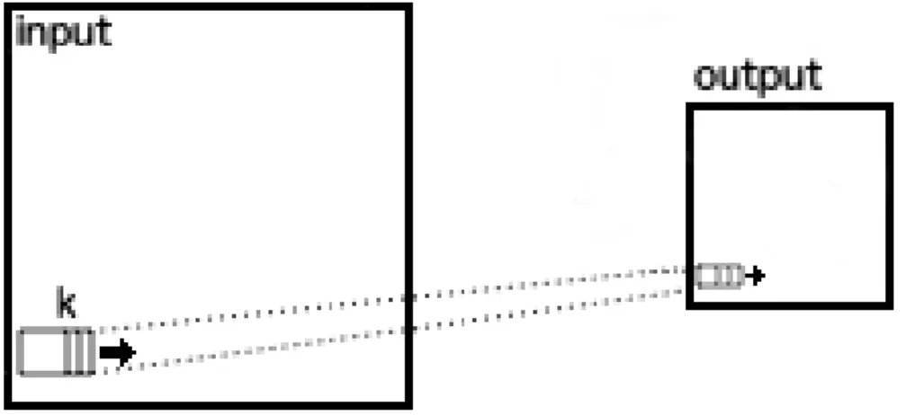
Convolutional layers calculate many products using a sliding window between the input

and the kernel, illustrated in Figure 2.3. The kernel is a set of 2-D weights that are adjusted

using the training process to respond to interesting geometric properties of the input images.

Each kernel functions as a feature detector. The sub-sampling layer either predominately

computes the average or maximum of a small neighborhood as illustrated in Figure 2.4.

The only difference is sub-sampling usually does not have overlap between neighborhoods.

Kernels learn to extract simple features through the lower layers, e.g. edges, and more

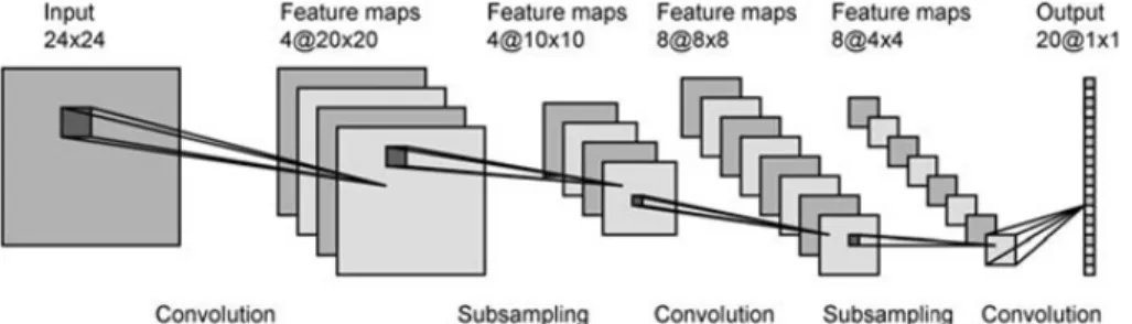
complex features in higher layers, e.g. faces. LeNet-5 [16], a typical CNN architecture

used for character recognition is shown in Figure 2.2.

Figure 2.2: Architecture of a typical simple Convolutional Neural Network. The network contains 2 convolution layers, 2 sub-sampling layers, and 2 fully connected layers. [16]

Figure 2.3: Convolution performed in the spatial domain. k represents the kernel. As k propagates through the input inner products are calculated. The result of these products generate the output.

Figure 2.4: Sub-sampling. The max is taken for each small neighborhood of values to generate the output. The neighborhoods do not overlap.

The output of a convolutional layer is referred to as a feature map. A feature is

cal-culated at each position in the map. This feature value is dependent on the input, kernel

and sub-sampling used, thus each feature is potentially different. Convolution can be

im-plemented sequentially, where each kernel is convolved with the pixels of the input using

a single neuron for each product and summing subsets of these neurons to simulate feature

maps. However, it is more efficient if the feature map is a plane of neurons that share a

single weight vector allowing convolution to be calculated in parallel. The sharing of the

more effectively. [16]

A convolutional layer usually produces multiple feature maps, all of which are

calcu-lated using different kernels. These kernels are usually initialized with normally distributed

random numbers based on the number of inputs and outputs in the layer [10]. Multiple

ker-nels are used to extract a variety of features associated with each location in an image.

The penultimate layer of a CNN is generally fully connected, comprising one output

for each class to be predicted. These outputs are fed into a softmax layer [1] that returns

a likelihood that the image belongs to any given class. The softmax was implemented to

allow the network to weigh its predictions in a probabilistic manner [1].

Large datasets are needed to learn meaningful features in a CNN. With small amounts

of data, over-fitting can become an issue [12]. Over-fitting happens when the network

optimizes directly to the training dataset and can no longer generalize to other data. A

common technique to increase the size of the dataset is data augmentation, where images

are rotated slightly, mirrored, or cropped differently. For example, from a 256 × 256 image, five 221× 221 images are cropped (four from the corners and one at the center), mirrored and rotated slightly. The amount of computations needed becomes larger due to

growing dataset sizes. With faster computers and the work performed in this thesis, CNNs

are becoming more efficient. [21]

CNNs share weights, meaning each kernel has its own set of weights and every

con-volution calculated with those kernels uses that set. In contrast, a fully connected layer

has a weight for every input-output combination. The sharing of weights causes fewer free

parameters in the network. Even with fewer free parameters CNNs can learn features that

preserve topology, localization, promote shift invariance, and effectively generalize. [16]

The convolutional layer has the ability to maintain and learn from the topology, the

way in which constituent parts are interrelated or arranged, of an image. For example, the

convolutional layer has the ability to learn a face based on the spatial arrangement of the

network achieve some scale invariance. [6]

Using the face example, convolutional layers preserve localization; if the eye is

con-tained in the northwest quadrant of the image the features representing the eye will be in the

northwest quadrant of the feature map. If the northwest quadrant of an unknown image’s

feature maps fail to show characteristics of an eye, the CNN kernels return low matching

values. Localization is achieved in a similar manner to topology: the feature map values

are generated from a local neighborhood of the input. [16]

Sub-sampling allows convolutional layers to be somewhat invariant to shift and

dis-tortion. Sub-sampling only allows the most predominate features in a neighborhood to

propagate through the layer, so even if the feature is shifted the network still propagates the

feature. If an image of a face is moved from a central location, the network may still be able

to identify the face. This is important in future research to ensure that objects occurring in

different locations in the images will be detected. Sub-sampling between the convolutional

layers only allows the maximum feature in a region to persist through the network. With

multiple sub-sampling layers, the features of interest propagate through the network even

if the distortion and/or shift move the important features from the region. [16]

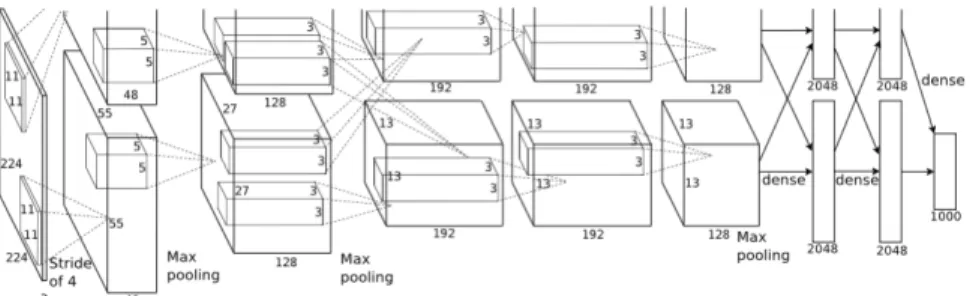
CNNs have shown recent success for classification tasks on popular datasets,e.g.

Im-ageNet. The network is composed of eight layers with weights. The first five layers are

convolutional and the last three are fully connected. The last layer is fed into a 1000 class

softmax layer. The network takes about a week to train and achieved state-of-the-art results

in 2012 for the ImageNet Classification Challenge. Table 2.1 compares the performance of

AlexNet on this dataset with that of previous state-of-the-art classifiers.

Wan Li recently developed a technique called DropConnnect [25] that adds to the

power of CNNs. Li reduced the error rate from 0.47% to 0.21% on MNIST (for more

Figure 2.5: Design of the Convolutional Neural Network AlexNet. This network has 5 convolutional layers, 3 sub-sampling layers, and 2 fully connected layers. [14]

Table 2.1: ImageNet result comparisons. The table lists previous classification attempts to compare to previous state-of-the-art systems. Top-1 is the error rate of the network only using the highest prediction, while top-5 is the error rate using the top 5 predictions made by the network. [14]

Table 2.2: DropConnect to non-DropConnect comparison using MNIST. [25]

AlexNet takes a week to train, and networks are still growing in size. CNNs need to

2.3

Convolution in the Frequency Domain

The Discrete Fourier Transform (DFT) utilizes circular convolutions. Withydefined as the

Hadamard product between DFT arraysXandHwe can use the inverse DFT to derive the

convolution operator. N represents the “circular convolution”. [7]

Consider: Y[k] =X[k]H[k] (2.1) Where: x[n]←−−−→DF T;N X[k] (2.2) h[n]←−−−→DF T;N H[k] (2.3) x[((n))N] def = 1 N N−1 X k=0 X[k]ej2πNkn (2.4)

Using the inverse DFT:

Y[n] = 1 N N−1 X k=0 H[k]X[k]ej2πNkn (2.5) = 1 N N−1 X k=0 N−1 X m=0 h[m]ej2πNkm ! X[k]ej2πNkn Commutative Property: = N−1 X m=0 h[m] " 1 N N−1 X k=0 X[k]ej2πNkn ! ej2πNkm # (2.6)

From equation 2.4 Y[n] = N−1 X m=0 h[m]x[((n))N]ej 2π Nkm (2.7) = N−1 X m=0 h[m]x[((n−m))N] =h[n] N x[n] h[n] N x[n] =h[n]∗x[((n)N] =h[n]∗ ∞ X l=−∞ x[n−lN] = ∞ X l=−∞ h[n]∗x[n−lN] Let: y[n] =h[n]∗x[n] (2.8)

Sum of shifted replicates:

y[n] =

∞

X

l=−∞

y[n−lN] (2.9)

Shifted replicates overlap if and only ify[n] ≤N. IfX[n]is durationMxandh[n]is

durationMhtheny[n] =h[n]∗x[n]is durationMy =Mx+Mn−1[7]. The length of the

arrayy[n]is required to beMy for circular convolution to equate linear convolution. For

2.4

Using FFT with Convolutional Neural Networks

Introducing the frequency domain to CNNs was done successfully by Mathieuet al. [18].

Mathieu uses a parallelized version of Cooley-Tukey Fast Fourier Transform Algorithm

[3] to allow for batches of FFTs to be performed in parallel. The work also explains how

2-D FFTs can be performed in a pair of 1-D transforms to greater parallelize the process.

Mathieu’s work states that convolution in frequency domain, a Hadamard product, is faster

than that of the traditional method.

Mathieu’s paper inspired this research which uses an existing FFT method in order to

create a frequency domain convolutional layer. Training is performed on networks using

convolutional layers that are propagated in the frequency domain to reiterate consistency

between the convolution methods. Different parameters of the layers are analyzed to show

the frequency domain implementation performance compared to the spatial convolution

and are presented in 4. Figure 2.6 is an illustration of the concept used to program the FFT

implementation of a CNN used both in Mathieuet al.and this thesis. [18]

Figure 2.6: Fast Fourier Transform Implementation from Mathieu [18]. Each convolu-tional layer must complete all illustrated calculations for each propagation in the forward direction. Matrix multiply refers to a hadamard product between the two vectors.

Table 2.3: Fast Fourier Transform Results from Mathieu 2013. Two neural network dis-tributions, Torch7 and CudaConv, are compared to the FFT convolution method. Each number represents the milliseconds taken to compute a single epoch of a CNN. [18]

2.5

Overlap-and-Add

In OaA, the input is broken intoN2_/n2_{blocks equal to the kernel size,n×n. A convolution}

between each block and the kernel is computed and the results are overlapped and added.

A 1-D example that generalizes to 2-D is shown in Figure 2.7. This figure illustrates a

simple 1-D overlap-and-add method for spatial convolution. The input is first split into

smaller blocks that are equal in size to the kernel. Smaller convolutions are then performed

between the kernel and the block inputs. The resulting convolutions are then added together

to create the same results as a traditional spatial convolution.

Each convolution in OaA can be efficiently computed in the frequency domain, where

the bottleneck is the complexity of each Fourier transformO(n2_log

2n). The total

com-plexity for the entire input and kernel is the number of blocks times the comcom-plexity of

each convolution, i.e. O(N2_log

2n). Table 2.4 compares the complexity of each

convolu-tion method, spaceConv refers to the tradiconvolu-tional convoluconvolu-tion in the space domain, FFTconv

refers to convolution via a Hadamard product in the frequency domain without

overlap-and-add, and OaAconv is the method we implement in our CNN design.

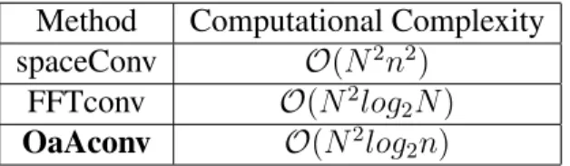
Method Computational Complexity spaceConv O(N2n2)

FFTconv O(N2log2N)

OaAconv O(N2_log 2n)

Table 2.4: Computational Complexity Comparison. spaceConv refers to the traditional convolution in the space domain, FFTconv refers to convolution via a Hadamard product in the frequency domain without overlap-and-add, and OaAconv is the method we implement in our CNN design.

When N n, as is the common case in CNN architectures, OaAconv reduces the computational complexity by a factor of _logn2

2nover spaceConv and by a factor of

logN

logn over

FFTconv. For example, for a 256 ×256 input array with a 5×5 kernel (typical values in a CNN architecture), spaceConv has a complexity of O(2562 ×25), FFTconv has a complexity ofO(2562×8), and OaAconv has a complexity ofO(2562×2.3).

The overall time complexity of OaAconv can be further reduced by noting that all

the block convolution can be computed in parallel. If N2 _{threads are available (a fair}

assumption for modern GPUs), the complexity on each thread isn2_log

2n, and the overall

time complexity is O(min(N2_{, n}2_log

2n)) which is usuallyO(N2). Additional speed up

can be obtained by taking advantage of the NVIDIA CUDA Fast Fourier Transform library

(cuFFT) that computes each FFTs up to 10x faster ([20] see also [24]). However, in order

to have a fair comparison, experiments in this paper are run on single threads.

A possible area of concern for OaA is the additional cost of breaking the input into

blocks and the cost of overlapping and adding after each convolution is computed. Our

experiments show an overall performance increase for the OaA technique despite these

overhead costs.

It is worth noting that although OaA theoretically reduces the computational

complex-ity in testing (and training), it is particularly beneficial in implementations such as Sermanet

et al.[22] when the test image is much larger than the training images, and testing requires

the use of a sliding window approach across a pyramid of scales for simultaneous detection

Figure 2.7: 1-D Overlap-and-Add convolutions. The kernel is convolved with the image. The image is split into subset that are equal in size to the kernel. Each subset is convolved with the kernel. The subset convolutions are overlapped then added together to produce the equivalent convolution. This example is done in the spatial domain, but the concept transfers to the frequency domain.

Methods

3.1

Problem Domain

The overall objective of this work is to improve the efficiency of CNNs by reducing the

computational expense of kernel convolution. The work described here is limited to

im-plementation of a CNN in the Fourier domain using traditional FFT and exploration of the

efficiency gains obtained using OaA for the convolution steps. Future work will be directed

at extracting more information from the network to improve classification accuracy.

The Mixed National Institute of Standard and Technology (MNIST) [17] dataset has

been chosen as a test platform to explore computational efficiency. MNIST contains 60,000

images in the training set and 10,000 images in the test set. The images are 28×28, grey-scaled, and contain a single handwritten numeric character. MNIST is a small datasets that

does not require much pre-processing. It was created for the purpose of testing machine

learning techniques. MNIST is available for no cost at http://yann.lecun.com/exdb/mnist/.

Many machine learning techniques exist that are accurate with less than 1% error rate using

MNIST. Examples can also be found at the URL given above. A set of images are presented

in Figure 3.1.

The images in MNIST were taken from the National Institute of Standard and

Tech-nology’s (NIST) special dataset. The numbers in the image are size normalized to 20×20 while preserving their aspect ratio. The character is centered at the center of mass of the

28. Reasoning for the normalization and size are given in Section 3.2.

Figure 3.1: Digits found in the MNIST dataset. There are multiple styles of the handwritten digits adding complexity to the task of classification.

3.2

System Design

A novel CNN was designed and implemented in order to compare spatial convolution to

the FFT and OaA methods. The same CNN design is used for comparisons between

space-Conv, FFTconv, and OaAconv. Pre-processed data is provided to two pairs of convolutional

sub-sampling layers. The output of the second sub-sampling layer is fed into two fully

connected layers designed to reduce the dimension of the output to match the number of

classes. Lastly, the second fully connected layer is fed into a softmax layer that expresses

the networks predictions in a probabilistic manner. The CNN implemented using spatial

net-work architecture, based on LeNet-5 [16]. Each of the CNN layers are discussed in detail

in the following subsections.

Figure 3.2: The MNIST digit is used as input into the first convolutional layer. The network contains 2 convolutional layers, 2 sub-sampling layers, and 2 fully connected layers. This architecture is used in experiment 1 found in Section 4.1. [16]

For the FFT implementation with no overlap-and-add, FFTconv, we use Fast Fourier

Transform in the West (FFTW) [9]. FFTW is the fastest implementation according to

the benchmarks ran, as shown in Figure 3.3. FFTW was picked based on performance

obtained by 2-D transformations of real data. The details on FFTconv are discussed further

in Section 3.2.3.

The OaA implementation, OaAconv, was also created using FFTW to allow for proper

comparisons between FFTconv and OaAconv. The design of OaAconv is discussed further

in Section 3.2.4.

3.2.1

Image Pre-processing

An example 28×28 image from the MNIST dataset is shown in Figure 3.4. The image is normalized to values between 0 and 1, inclusive. The normalization is performed to keep

Figure 3.3: Benchmarks calculated for different implementations of an FFT. All implemen-tations are tested on double-precision real-data 2-D transforms. Each method is tested at differing transform sizes. FFTW3 provides the overall fastest transforms. [8]

When the exponential of the output is larger than 4 bytes NaNs are created in the softmax

layer.

Figure 3.4: A single input image from MNIST. [15]

3.2.2

spaceConv Method

The first convolutional layer uses the normalized image as input, size 28 ×28, and con-volves with 20 kernels of size 5×5. The layer uses a weight vector of 5×5×20, as each kernel has its own weight vector. All convolutional layers have a stride of 1, meaning the

sliding window moves 1 pixel after each calculation. The stride results in input size minus

24×20 feature map. With no non-linearity, the output is sent to the first max sub-sampling layer. Max sub-sampling is performed with a 2×2 neighborhood to reduce the output size to 12×12×20. There are 50 kernels of size 4×4 in the next layer. The weight vector is sized 4×4×20×50 as each input depth and kernel receives its own weight vector. After going through the convolutional layer the 9 × 9× 50 feature map is fed into the second sub-sampling layer. The second max sub-sampling layer uses a neighborhood of 3×3 and produces a result of 3×3×50. This network is illustrated in Figure 3.5.

The backward propagation of the convolutional layer calculates two different values,

change in weights and error. Change in weights is the result of a convolution of the previous

error with the input. The learning rate controls the speed at which the weights change. The

error calculation is a convolution between the weight vector and the previous errors. The

weight vectors are inverted so the convolution equates to the derivative calculation used for

the backward propagation.

The sub-sampling layer has no weight vector; therefore there is no change in weights

to calculate. The sub-sampling layer has multiple possible types, each of which have

differ-ent backward propagations. Max sub-sampling propagates the error backward to the neuron

that produced the max activation during the forward propagation. Average sub-sampling

propagates an average of the error to all locations in the neighborhood used to calculate the

average. The first and second convolutional layers can

3.2.3

FFTconv Method

For the forward propagation the convolution is performed between the input and the kernel.

Padding must be performed to ensure the FFT calculates the full convolution. The images

must be padded to the size of the input image plus the size of the kernel minus one. The

kernel vector is inverted before the padding because convolutional layers actual calculate

Figure 3.5: Convolutional layers of the CNN. The first convolutional layer uses 20 kernels to generate feature maps of size 24× 24× 20. The first sub-sampling uses a maximum neighborhood to reduce the feature maps to size 12×12×20. The second convolutional layer uses 50 kernels to calculate kernel maps of size 9×9×50. The second sub-sampling layer uses a max neighborhood to reduce the feature maps to size 3×3×50. [15]

The input vector is transformed for each input depth and the kernel vector is transformed

for each input and kernel. The Hadamard product is calculated and the sum is calculated

over the input depths for each kernel. These calculations can be performed simultaneously.

The IFFT is computed on the resulting vector and is cropped to the proper output size:

Figure 3.6 illustrates the forward propagation for FFTconv excluding padding.

Figure 3.6: FFTconv Forward Propagation. LetDandNk be the input depth and number

of kernels, respectfully. FFTs are performed on the kernels and the inputs. A Hadamard product is calculated between the resulting vectors. An IFFT is performed on the product to produce the convolution.

the deltas, a variable used in propagation which equates to the errors multiplied by the

derivative of the non-linearity, is equivalent to the errors. The change in weights convolves

the input with the deltas and is illustrated in Figure 3.7. The inputs and deltas are padded to

the size of the inputs plus the deltas, output size, minus one. The deltas are inverted before

padding in order to cause the convolution to be calculated correctly using the FFT. The FFT

for the deltas requires the same number of transforms as the number of kernels employed,

and the inputs require the same number of transforms as the input depth employed. The

Hadamard product is calculated between the padded inputs and deltas. The inverse FFT is

computed on the resulting vector and is cropped to the size of the weights. During each

propagation the system keeps track of the error, and after, the mini-batch the entire error is

accounted for with a single backward propagation.

Figure 3.7: FFTconv Weight Change Propagation. Let Dand Nk be the input depth and

number of kernels, respectfully. FFTs are performed on the inputs and the deltas. A Hadamard product is calculated between the resulting vectors. An IFFT is performed on the product to produce the convolution.

The second convolution in the backward propagation calculates the resulting error of

the layer, illustrated in Figure 3.8. Error is calculated by convolving the delta with the

weight vectors. Both vectors are padded to the size of deltas plus the size of weights minus

one. The weight vector is inverted for the original calculation of the error in non-FFT

Hadamard product is calculated between the two vectors and is summed over the kernels

for each input depth. The inverse FFT requires the same number of transforms as the input

depth employed on the resulting vector and is cropped to be the desired size. If the layer

is the first in the network then the errors can be used to judge the confidence the network’s

predictions.

Figure 3.8: FFTconv Error Propagation. Let D, Nk be the input depth and number of

kernels, respectfully. FFTs are performed on the weights and the deltas. A Hadamard product is calculated between the resulting vectors. An IFFT is performed on the product to produce the convolution.

3.2.4

OaAconv Method

OaAconv does more transforms that are smaller in size compared to FFTconv. The input is

first padded so that it is evenly divisible by the kernel. Then the input is divided into

sub-sections of the kernel size. Each sub-section and the kernels are padded to the size of double

the kernel minus 1. Each of these padded sub-sections and padded kernels are transformed.

The Hadamard product is calculated and the IFFTs are computed. The results must be

assembled with an overlap of kernel size minus one. Overlap is needed to produce the

correct inner product, causing equivalence in the convolution methods. After the overlap is

Figure 3.9: OaAconv Forward Propagation. LetD,Nk, andNdbe the input depth, number

of kernels, and number of divisions, respectfully. FFTs are performed on the kernels and the subdivided inputs. A Hadamard product is calculated between the resulting vectors. An IFFT is performed on the product, overlapped, and added to produce the convolution.

The change in weight convolves the inputs and the deltas. The sub-sections of the

input are equal to the size of the deltas and are padded to two times the delta size minus

one. These sub-sections are transformed, convolved, IFFTed, and reassembled with an

overlap of deltas minus one. The error calculation uses a kernel with the size of the deltas.

The sub-sections of the weight vector are equal to the size of the deltas and are padded to

twice the size of the deltas minus one. The sub-sections and weight vectors are transformed;

the weights are theoretically inverted twice, so in practice the vector is not inverted at all.

The Hadamard product is calculated and the results are summed over the kernels. The

IFFT is computed, then reassembled with a kernel size minus one overlap and cropped to

the correct size. Figure 3.10 represents the weight change for OaAconv and Figure 3.11

illustrates the error propagation for OaAconv.

3.2.5

Fully Connected Layer

The last sub-sampling layer feeds directly into the first fully connected layer. The input is

input-Figure 3.10: OaAconv Weight Change Propagation. LetD,Nk, andNdbe the input depth,

number of kernels, and number of divisions, respectfully. FFTs are performed on the deltas and the subdivided inputs. A Hadamard product is calculated between the resulting vectors. An IFFT is performed on the product, overlapped, and added to produce the convolution.

Figure 3.11: OaAconv Error Propagation. LetD, Nk, andNd be the input depth, number

of kernels, and number of divisions, respectfully. FFTs are performed on the deltas and the subdivided weights. A Hadamard product is calculated between the resulting vectors. An IFFT is performed on the product, overlapped, and added to produce the convolution.

output combo and a bias for each output. The weights are initialized based on the number

of inputs and outputs [10]. The change of weights use the same learning coefficient as

the convolutional layer to control learning. The bias learns twice as fast as the weights,

achieved by doubling the learning rate.

The first fully connected layer feeds into a ReLU non-linearity, which allows the

out-put to proceed if positive, else the outout-put is 0. This outout-put is fed into another fully connected

The second fully connected layer follows the same parameters as the first, including the

learning rate.

The non-linearity is used after each fully connected layer, meaning the previous error

must only propagate through the network if the forward propagation was positive. The

local gradient is the product of the derivative of the ReLU and the previous error. The

local gradient is multiplied by the weights to produce the errors of the layer. The change

in weights are calculated by multiplying the local gradient with the input and the learning

rate. The change in the bias is the product of the learning rate and the local gradient.

3.2.6

Softmax Layer

The output of the second fully connected layer is fed into a softmax layer. The softmax

layer returns the quotient of the exponential of the current output divided by the sum of the

exponential of all outputs. The softmax layer output equates to the class-wise probabilities

produced by the network’s predictions. The softmax layer produces weighted results that

can be properly evaluated with a simple cost function.

These probabilities are fed into the cost function, which when combined with the

backward propagation of the softmax layer is calculated by subtracting the desired results

from the calculated probabilities. This error is propagated backward through the network

to calculate weight changes.

3.3

System Complexity

The complexity described in Table 2.4 is the reduced BigO Notation. The forward prop-agation of FFTconv has two FFTs and one IFFT, along with the Hadamard product. The

padding is ignored as an optimal implementation would already include the padding before

input depth, number of kernels, and number of divisions, respectfully. For the forward

propagation of the network,N =Si+Sk−1. The first FFT for the input has a complexity

ofO(D∗N2_log

2(N)). The kernel transform has complexityO(Nk∗D∗N2log2(N)). The

Hadamard product of the resulting vectors has complexityO(D∗Nk∗N2). To reduce the

number of IFFTs the vector is summed over input depth giving,O(Nk∗N2log2(N)). The

entire forward propagation results in a complexityO((D+ (Nk∗D) +Nk)∗N2log2(N) +

(Nk∗D∗N2)), which reduces toO(N2log2(N)).

The backward propagation contains four FFTs and two IFFTs. For the calculation

of weight changes N∆w = Si +So −1. The FFT on the input has a complexityO(D∗ N2

Elog2(N∆w)). The deltas are then transformed, which has complexityO(Nk∗N∆2wlog2(N∆w)).

A Hadamard product is calculated between the results, giving a complexity O(D∗Nk ∗ N_∆2_w). The IFFT is calculated on the result from the Hadamard product, O(D ∗ Nk ∗ N_∆2_wlog2(N∆w)).

The backward propagation also needs to calculate the error. For this calculation,

NE =Sk+So−1. The FFT for the kernels is,O(D∗Nk∗NE2log2(NE)). The deltas are

transformed,O(Nk∗NE2log2(NE)). AsNE is a different size thanN∆win the two

calcula-tions, the transform does need to be performed again. The Hadamard product is calculated

between the two FFTs, O(D∗Nk ∗NE2), and is summed over the kernels. The IFFT is

then calculated, O(D∗N_E2log2(NE)), giving the errors to propagate. In combination the

complexity of the backward propagation is: O((D+Nk+ (D∗NK))∗N∆2wlog2(N∆w)) + (D+NK+ (D∗NK))∗NE2log2(NE)) + (Nk∗D∗N∆2w) + (Nk∗D∗NE2)). This reduces

toO(N2_log

2(N)), whereN ismax(N∆w, NE).

OaAconv has a complexityO(N2_log

2(N)). For the forward propagation N is equal

to the size of the image and n is equal to the size of the kernel. The first FFT is for

the input and has a complexityO(D∗Nd∗N2log2(N)). The number of divisions is the

number of sub-sections the input is divided into, which is the input divided by the kernel

calculated on the results,O(Nk∗D∗Nd∗n2). To reduce the size of the IFFT the input

depth is summed over, O(Nk ∗ Nd ∗ N2log2(N)). The results from the IFFT are then

reassembled, O(Nd∗n2). The entire forward propagation using OaS gives a complexity

O(((D∗Nd) + (D∗Nk))∗N2log2(N) + (Nd+ (D∗Nk∗Nd))∗n2)). This complexity

reduces toO(N2log2(N)).

The backward propagation for OaAconv has multiple convolutions. Ni in this case is

equal to the input size, andnois equal to the output size. The deltas are transformed with a

complexityO(Nk∗Ni2log2(no)). The input is transformed,O(D∗Nd∗Ni2log2(no)), where Ndis the times the output size goes into the input size. A Hadamard product is calculated

between the two FFTs, O(Nd ∗D ∗Nk ∗n2o). No summation is performed during this

process. The output from the product is now reassembled to getO(D∗n2

o).

The error propagation convolution is performed between the kernels and the deltas.

No is equal to the output size andnk is representative of the size of the kernels. FFTs are

calculated for the kernels and deltas,O(D∗Nk∗No2log2(nk))andO(Nk∗Nd∗No2log2(nk)),

respectively. The Hadamard product is calculated, O(D ∗Nk ∗Nd∗ n2k), and summed

over the kernels to reduce the IFFT. The IFFT and reassembly are of complexityO(D∗

Nd∗No2log2(nk))andO(Nd∗n2k), respectively. The complete complexity of OaAconv’s

backward propagation is O((Nk+ (D∗Nd))∗Ni2log2(no)) + ((Nk∗D) + (D∗Nk))∗ N_o2log(n2_k)) + (((Nd∗D∗Nk) +Nd)∗n2o) + ((D∗Nk∗Nd) +Nd)∗n2k)). This complexity

Analysis

4.1

Training Consistency

Question one of this thesis is to determine if spaceConv, FFTconv, and OaAconv are

em-pirically equivalent. This will determine if OaAconv is directly interchangeable with the

traditional spatial convolution. This experiment has not been shown in the literature. In

this experiment we use each method of convolution to train the CNN designed in Chapter

3 using the MNIST [17] dataset. The premise of this experiment is to determine if the

methods are empirically equivalent. Each network is trained for only 100 epochs as that is

sufficient to demonstrate consistency. Each CNN network is trained five times with each

type of convolution technique, and their classification rate averages are shown in Table 4.1.

As expected, all three methods had an accuracy rate that averaged within 0.1% of each

other. The differences can be explained by the random parameter initialization in training

each CNNs. Table 4.2 shows results of training each of the CNNs in a non-stochastic

Method Training 1 Training 2 Training 3 Training 4 Training 5 Average spaceConv 91.98% 92.38% 92.21% 92.81% 93.01% 92.48% FFTconv 92.46% 92.29% 91.79% 93.14% 92.37% 92.41% OaAconv 93.21% 92.52% 92.73% 91.81% 92.01% 92.46%

Table 4.1: 100 Epoch Training Results for each Layer Type. The values represent clas-sification accuracy on MNIST for each convolution method. All three methods generate similar results.

Method Training 1 Training 2 Training 3 Training 4 Training 5 Average spaceConv 86.37% 86.37% 86.37% 86.37% 86.37% 86.37% FFTconv 86.37% 86.37% 86.37% 86.37% 86.37% 86.37% OaAconv 86.37% 86.37% 86.37% 86.37% 86.37% 86.37%

Table 4.2: 100 Epoch Non-stochastic Training Results for each Layer Type. The values represent classification accuracy on MNIST for each convolution method. All three meth-ods generate the same exact results

process. The non-stochastic process has the same weights initialized for all tests and no

randomness in the order of the images used for training.

4.2

Time vs. Number of Kernels and Input Depth

To determine if the initialization cost of OaAconv is computationally too expensive the

number of transforms is varied. If OaAconv does not overcome the extra initialization cost,

the method does not provide any use. In this experiment we compare the required total

propagation time through one convolutional layer as the number of kernels in the layer

increases. The input array is of size 32 × 32 and each kernel is of size 5 × 5. Figure 4.1 shows the speed-up factor of FFTconv and OaAconv compared to spaceConv in the

forward propagation of the convolutional layer as the number of kernels varies. The number

of kernels is varied from 25 to 750 with a discrete step of 25. Each “number of kernels”

experiment is replicated 10 times and the results are averaged.

FFTconv and OaAconv outperform spaceConv, and OaAconv outperforms FFTconv

at every step. FFTconv and OaAconv have an additional initialization cost: in OaA the

input array must be divided, and in both methods the input (or divided input) array and

kernel must be zero-padded prior to computing the Fourier transforms. As the number of

kernels increases, these additional initialization costs becomes less significant.

Figure 4.1: Speed-up over spaceConv vs. Number of Kernels in Forward Propagation. As the number of kernels increases the initialization cost becomes less significant.

propagation. Our method outperforms FFTconv more than in the forward propagation. The

reason for this is that the backward propagation contains two actual convolutions per kernel:

one convolution to propagate the error through the layer and another to calculate the change

in weight generated by this error.

These experiments show that the additional initialization costs of using OaAconv and

FFTconv are mitigated by the lower complexity of these methods. The more kernels used,

the larger the performance increase of our method.

4.3

Time vs. Kernel size

To determine if the method is consistent with the theoretical complexities the impact of the

kernel size must be tested. In this experiment we vary the size of the kernel while keeping

Figure 4.2: Speed-up over spaceConv vs. Number of Kernels in Backward Propagation. As the number of kernels increases the initialization cost becomes less significant.

is held constant at 100. Figures 4.3 and 4.4 show the speed-up over spaceConv vs. kernel

size for the forward and backward propagation, respectively. The kernel sizes vary from

1 to 64 with a discrete step of 1. Each experiment is repeated 10 times and the results are

averaged.

In the forward propagation in Figure 4.3, the performance of FFTconv and OaAconv

converge at 64 as expected. An interesting aspect of this result is the various performance

peaks at different kernel sizes. This is because the FFT software [9] is optimal for Fourier

transforms where the size of each dimension is an even power of two. We can leverage

this fact when designing CNN architectures to further reduce computational requirements.

Note that the backward propagation has peak performances at different kernel sizes due to

Figure 4.3: Speed-up over spaceConv vs. Kernel Size in Forward Propagation. As the kernel size increases the OaAconv and FFTconv converge. Peaks are formed due to FFTW performance while using transforms of sizes that are powers of two.

4.4

Time vs. Input Size

To determine if the method is consistent with the theoretical complexities the impact of

the image size is tested. In this experiment we test the performance of multiple input sizes

while holding the kernel size constant at 5 × 5. According to the complexity, OaAconv outperforms FFTconv for small kernel sizes. The input sizes varied from4×4to256×

256 with a discrete step of 4×4 for the forward propagation experiment and a discrete step of 8×8for the backward propagation experiment. Each “input size” experiment is replicated 10 times and the results are averaged. Figures 4.3 and 4.6 show the speed-up

over spaceConv vs. input size for the forward and backward propagation, respectively.

Figure 4.4: Speed-up over spaceConv vs. Kernel Size in Backward Propagation.As the kernel size decreases the OaAconv and FFTconv converge. Peaks are formed due to FFTW performance while using transforms of sizes that are powers of two.

speed-up in the backwards propagation is more significant. The error propagation is greatly

Figure 4.5: Speed-up over spaceConv vs. Input Size in Forward Propagation. With a constant small kernel OaAconv outperforms FFTconv. FFTconv has minor peaks due to FFTW calculating transforms efficiently that are powers of two in size.

Figure 4.6: Speed-up over spaceConv vs. Input Size in Backward Propagation. With a constant small kernel OaAconv outperforms FFTconv. FFTconv has minor peaks due to FFTW calculating transforms efficiently that are powers of two in size.

Conclusion

Results of the experiments in Chapter 4 are summarized in Table 5.1. The best results from

each experiment are given.

Method Number of Kernels and Input Depth Kernel Size Image Size

FFTconv 3.4 27.3 3.7

OaAconv 4.3 50.4 25.8

Table 5.1: Max Speed Ups

This thesis addresses three questions. First if FFTconv and OaAconv produce

classi-fication results consistent with results produced using spaceConv. The result presented in

Section 4.1 clearly shows that this is true. According to the theory: every method used to

train the CNN results in the same output of convolutional operators, which is empirically

demonstrated.

The second question asked if OaAconv and FFTconv are faster even with the extra

overhead of FFT transforms being performed at the start and end of each layer’s

propa-gation step. Sections 4.2 - 4.4 show different parameters where the increase in speed is

substantial. Both methods can be developed to reduce the initialization cost and be run in

parallel.

The last question asks if OaAconv outperforms FFTconv. OaAconv can allow Neural

Networks to use small kernels on large images to improve learning of information. Sections

4.2 - 4.4 show that OaAconv is a more efficient method than FFTconv.

used. OaAconv has a large amount of untapped power in parallel computing as each of

the transforms can be calculated separately and in conjunction with one another. Future

work includes implementing OaAconv on a graphics processing unit(GPU). The future

im-plementation will no longer use FFTW as the transforms are optimal at 64×64. The best FFT for OaAconv needs to be optimized for transforms of 8×8.

Bibliography

[1] Christopher M Bishop et al. Pattern recognition and machine learning, volume 4.

springer New York, 2006.

[2] Bing Cheng and D Michael Titterington. Neural networks: A review from a statistical

perspective. Statistical science, pages 2–30, 1994.

[3] James W Cooley and John W Tukey. An algorithm for the machine calculation of

complex fourier series. Mathematics of computation, 19(90):297–301, 1965.

[4] Navneet Dalal and Bill Triggs. Histograms of oriented gradients for human

detec-tion. In Computer Vision and Pattern Recognition, CVPR. IEEE Computer Society

Conference on, volume 1, pages 886–893. IEEE, 2005.

[5] Jia Deng, Wei Dong, Richard Socher, Li-Jia Li, Kai Li, and Li Fei-Fei. Imagenet: A

large-scale hierarchical image database. InComputer Vision and Pattern Recognition,

CVPR. IEEE Conference on, pages 248–255. IEEE, 2009.

[6] John S Denker, Richard E Howard, Lawrence D Jackel, and Yann LeCun.

Hierarchi-cal constrained automatic learning neural network for character recognition,

Septem-ber 10, 1991. US Patent 5,067,164.

[7] Paulo SR Diniz, Eduardo AB Da Silva, and Sergio L Netto.Digital signal processing:

[8] Matteo Frigo and Steven G Johnson. Benchfft.

[9] Matteo Frigo and Steven G Johnson. Fftw: An adaptive software architecture for

the FFT. InAcoustics, Speech and Signal Processing. Proceedings of the 1998 IEEE

International Conference on, volume 3, pages 1381–1384. IEEE, 1998.

[10] Xavier Glorot and Yoshua Bengio. Understanding the difficulty of training deep

feed-forward neural networks. In International conference on artificial intelligence and

statistics, pages 249–256, 2010.

[11] Geoffrey E Hinton and Ruslan R Salakhutdinov. Reducing the dimensionality of data

with neural networks. Science, 313(5786):504–507, 2006.

[12] Anil Jain and Douglas Zongker. Feature selection: Evaluation, application, and small

sample performance. Pattern Analysis and Machine Intelligence, IEEE Transactions

on, 19(2):153–158, 1997.

[13] Alex Krizhevsky and Geoffrey Hinton. Learning multiple layers of features from

tiny images.Computer Science Department, University of Toronto, Tech. Rep, 1(4):7,

2009.

[14] Alex Krizhevsky, Ilya Sutskever, and Geoffrey E Hinton. Imagenet classification with

deep convolutional neural networks. In Advances in neural information processing

systems, pages 1097–1105, 2012.

[15] B Boser Le Cun, John S Denker, D Henderson, Richard E Howard, W Hubbard, and

Lawrence D Jackel. Handwritten digit recognition with a back-propagation network.

InAdvances in neural information processing systems. Citeseer, 1990.

[16] Yann LeCun and Yoshua Bengio. Convolutional networks for images, speech, and

[18] Michael Mathieu, Mikael Henaff, and Yann LeCun. Fast training of convolutional

networks through FFTs. arXiv preprint arXiv:1312.5851, 2013.

[19] Vinod Nair and Geoffrey E Hinton. Rectified linear units improve restricted

boltz-mann machines. In Proceedings of the 27th international conference on machine

learning (ICML-10), pages 807–814, 2010.

[20] CUDA Nvidia. Cufft library, 2010.

[21] David E Rumelhart, Geoffrey E Hinton, and Ronald J Williams. Learning internal

representations by error propagation. Technical report, DTIC Document, 1985.

[22] Pierre Sermanet, David Eigen, Xiang Zhang, Micha¨el Mathieu, Rob Fergus, and Yann

LeCun. Overfeat: Integrated recognition, localization and detection using

convolu-tional networks. arXiv preprint arXiv:1312.6229, 2013.

[23] Christian Szegedy, Wei Liu, Yangqing Jia, Pierre Sermanet, Scott Reed, Dragomir

Anguelov, Dumitru Erhan, Vincent Vanhoucke, and Andrew Rabinovich. Going

deeper with convolutions. arXiv preprint arXiv:1409.4842, 2014.

[24] Nicolas Vasilache, Jeff Johnson, Michael Mathieu, Soumith Chintala, Serkan

Pi-antino, and Yann LeCun. Fast convolutional nets with fbfft: A gpu performance

evaluation. arXiv preprint arXiv:1412.7580, 2014.

[25] Li Wan, Matthew Zeiler, Sixin Zhang, Yann L. Cun, and Rob Fergus. Regularization

of neural networks using dropconnect. In Sanjoy Dasgupta and David Mcallester,

edi-tors,Proceedings of the 30th International Conference on Machine Learning

(ICML-13), volume 28, pages 1058–1066. JMLR Workshop and Conference Proceedings,