Multi-dimensional Point Process Models in
R
Roger D. Peng
Department of Statistics, University of California, Los Angeles
Los Angeles CA 90095-1554
Abstract
A software package for fitting and assessing multi-dimensional point process models using theR sta-tistical computing environment is described. Methods of residual analysis based on random thinning are discussed and implemented. Features of the software are demonstrated using data on wildfire occurrences in Los Angeles County, California and earthquake occurrences in Northern California.
1
Introduction
This paper introduces anRpackage for fitting and assessing multi-dimensional point process models. In par-ticular, the software is designed for conducting likelihood analysis of conditional intensity models. While the methodology for applying maximum likelihood to point process models is already well-developed, techniques for assessing the absolute goodness-of-fit of models are still being actively researched. We describe several methods ofpoint process residual analysissuch as random rescaling, thinning, and approximate thinning, and discuss their advantages and disadvantages in practice. The package implements two random thinning-based methods.
Section 2 begins with a brief discussion of the specification and fitting of point process conditional inten-sity models. Section 3 describes several residual analysis techniques and discusses their various properties. Section 4 describes some existing Rpackages for analyzing point data and Section 5 describes the ptproc package. In particular, we show how features of the R language such as lexical scope and the ability to manipulate language objects are used to build a compact flexible framework for analyzing point process models. Finally, Section 6 shows two extended examples of how one might use theptprocpackage.
The current version (1.4) of ptprocwas written and has been tested withRversion 1.7.1. The package is written in pureRcode so it should be usable by anyone with access to anRinterpreter.
2
Point Process Models
A point process can be thought of as a random measureN specifying the number of points, N(A), in any compact setA⊂S, whereS is simply the domain in which the point process resides. The measure is non-negative integer-valued and is finite on any finite subset ofS. Usually, one assumes that the point process is
simple, so that each point is distinct with probability one. For the purposes of this paper, we will only look at simple point processes in the space-time domain (i.e. S⊂R3), with one time dimension and two spatial dimensions.
A simple point process is conveniently specified by its conditional intensity λ(t,x) ((t,x)∈S), defined as the limiting expectation,
lim ∆t↓0 ∆x↓0
1
∆t∆xE[N((t, t+ ∆t)×(x,x+ ∆x))|Ht]
where Ht represents the internal history of the process up to time t and N((t, t+ ∆t)×(x,x+ ∆x)) is the number of points in a small neighborhood of (t,x). When it exists, the conditional intensity can be interpreted as the instantaneous rate of occurrence of events at timet and locationx.
Since the conditional intensity completely specifies the finite dimensional distributions of the point pro-cessN (Daley and Vere-Jones, 1988), modellingN typically involves directly modellingλ. Many conditional intensity models have been developed for specific applications, most significantly from the field of seismol-ogy (e.g. Vere-Jones, 1970; Ogata, 1999) and also ecolseismol-ogy (Rathbun and Cressie, 1994b).
2.1
Model Fitting
Given a parametrized model for the conditional intensity (with parameter vectorθ), the unknown parameters can be estimated by maximizing the log-likelihood function
`(θ) = Z S logλ(t,x;θ)N(dt, dx)− Z S λ(t,x;θ)dt dx (1)
It has been shown that under general conditions, the maximum likelihood estimates are consistent and asymptotically normal (Ogata, 1978; Rathbun and Cressie, 1994a; Rathbun, 1996). When maximizing the log-likelihood, care must be taken to ensure that λ is positive at all points in S. One solution to this potential difficulty is to model logλ rather than model λ directly (see e.g. Berman and Turner, 1992). Another method is to include a penalty in the specification of the log-likelihood which penalizes against parameter values which produce negative values of the conditional intensity. For example, one could use the following modified log-likelihood function
`∗(θ) =`(θ)−P(θ)
whereP(θ) is a suitable penalty function. For example, one could use a smooth penalty function as in Ogata (1983). An alternative would be simply to add a penalty any time the conditional intensity takes a negative value. Given an appropriateα >0, let
P(θ) =α1{λ(t,x;θ)<0, (t,x)∈S} (2)
where1{A} is the indicator of the eventA.
3
Residual Analysis Methods
A common method of evaluating a point process model is to examine likelihood criteria such as the Akaike Information Criterion or the Bayesian Information Criterion (e.g. Ogata, 1988; Ogata and Tanemura, 1984; Vere-Jones and Ozaki, 1982). These criteria provide useful numerical comparisons of the global fit of com-peting models. For example, a common model for comparison is the homogeneous Poisson model. However,
these criteria cannot shed light on the absolute goodness-of-fit of a particular model. In particular, they cannot identify where a model fits poorly and where it fits well.
Residual analysis in other statistical contexts (such as regression analysis) is a powerful tool for locating defects in the fitted model and for suggesting how the model should be improved. While the same is true in point process analysis, one must be careful in how one defines the residuals in this context. For point processes the “residuals” consist of yet another point process, called theresidual process. There exist various ways of constructing a residual process and we discuss some of those methods in this Section.
The common element of residual analysis techniques is the construction of an approximate homogeneous Poisson process from the data points and an estimated conditional intensity function ˆλ. Suppose we observe a one-dimensional point process t1, t2, . . . , tn with conditional intensity λ on an interval [0, T]. It is well
known that the points
τi=
ti Z
0
λ(s)ds (3)
fori= 1, . . . , n form a homogeneous Poisson process of rate 1 on the interval [0, n]. This new point process
is called the residual process. If the estimated model ˆλ is close to the true conditional intensity, then the residual process resulting from replacingλwith ˆλin (3) should resemble closely a homogeneous Poisson process of rate 1. Ogata (1988) used this random rescaling method of residual analysis to assess the fit of one-dimensional point process models for earthquake occurrences. For the multi-one-dimensional case, Schoenberg (1999) demonstrated that for a large class of point processes, the domain can be rescaled in such a way that the resulting process is again homogeneous with rate 1.
When rescaling a multi-dimensional point process one may encounter two practical difficulties:
1. The boundary of the rescaled domain may be uninterpretable (or unreadable). That is, the residual process may be homogeneous Poisson but the irregularity of the rescaled domain can make the points difficult to examine. In particular, an irregular boundary can bias various tests for uniformity which are sensitive to edge effects.
2. Integration of the conditional intensity function is required. In practice, accurate integration of the conditional intensity in certain dimensions can be computationally intensive.
Both of these problems can be ameliorated by instead constructing a residual process via random thinning. Suppose that for all (t,x)∈S there exists a valuemsuch that
0< m≤ inf
(t,x)∈Sλ(t,x). (4)
Then for eachi= 1, . . . , n, we delete the data point (ti,xi) with probability 1−m/λ(ti,xi). The undeleted
points form a homogeneous Poisson process of rate m over the original domain S. The residual process obtained through this method of thinning will be referred to as the ordinary thinned residual process or
ordinary thinned residuals. For details on random thinning, see Lewis and Shedler (1979) and Ogata (1981). To construct the ordinary thinned residual process, we only need to evaluate the conditional intensity. Typically, this is a much simpler task than integrating the conditional intensity. Unfortunately, in some cases wheremis very close to zero, the thinning process can result in very few points. However, because of the randomness involved in the thinning procedure, one can repeat the thinning many times and examine the various realizations for homogeneity. Another drawback of this method is that there may not exist such anm.
A third method for constructing a residual process addresses the problem of having too few points in the thinned process. Each data point (ti,xi) is assigned a probabilitypi such that
pi∝ 1
λ(ti,xi)
.
Then, a weighted subsample of sizeK(< n) is drawn from the vector{(t1,x1), . . . ,(tn,xn)}using the weights
p1, . . . , pn. As long asKis sufficiently small relative ton, the resulting set of points{(t∗1,x∗1), . . . ,(t∗K,x∗K)}
should resemble (approximately) a homogeneous Poisson process of rate K/kSk over the original domain. The process constructed using this method will be referred to as theapproximate thinned residual process, or simplyapproximate thinned residuals. This procedure can also be used to generate many realizations of the residual process and each realization will have exactlyK points. Approximate thinned residuals were used in Schoenberg (2003) to assess the space-time Epidemic-Type Aftershock Sequence model of Ogata (1998).
The residual process is useful for model evaluation purposes because the process is homogeneous Poisson if and only if the model is equal to the true conditional intensity function. Once the residual process has been constructed, it can be inspected (graphically) for uniformity and homogeneity. In addition, numerous statistical tests can be applied to test the process for uniformity (see e.g. Diggle, 1983; Ripley, 1979, and many others). For example, Ripley’sKfunction can be used to test for spatial clustering and inhibition (Rip-ley, 1976). In general, any deviation of the residual process from a homogeneous Poisson process can be interpreted as a deviation of the model from the true conditional intensity.
4
Point Process Packages for
R
There are already a fewRpackages available on CRAN for analyzing point data. Some notable ones include
the spatstat package of Baddeley and Turner and the splancs package of Rowlingson, Diggle, Bivand,
and Petris. These packages are largely concerned with analyzing two-dimensional point patterns. The
spatstat package of Baddeley and Turner provides data structures and functions for fitting a variety of
spatial statistical models via maximum pseudolikelihood. In particular they use a novel approximation to construct a simple method for maximizing the pseudolikelihood (see Baddeley and Turner, 2000). The authors’ concentration on purely spatial patterns (and the associated models) allows for the inclusion of many useful functions and utilities, all related to spatial analysis. In general, the user does not have to write much code in order to take advantage of the model fitting routines.
Thesplancslibrary is another package for two-dimensional point patterns (see Rowlingson and Diggle,
1993, for details). This package contains many useful functions for computing spatial statistics over irregular boundaries, simulating point patterns, and doing kernel smoothing. The package has less of an emphasis on model fitting thanspatstat. Some code for analyzing space-time data is available in the package, e.g. functions for computing space-timeK-functions (Diggle et al., 1995).
The choice of package to use will obviously depend on the needs of the user. The package discussed here is intended to be somewhat more general than those concerned with purely spatial point patterns. However, to achieve this greater generality, much of the burden of writing code has been shifted to the user. In particular, we discuss in Section 5 how the user must write code for evaluating and integrating the conditional intensity. The primary goal for this package is to provide a general framework for organizing multi-dimensional point process data and fitting arbitrary conditional intensity models. In addition, we provide tools for model doing model assessment and point process residual analysis.
5
The
ptproc
Package
Theptprocsource package and updates can be downloaded from the UCLA Department of Statistics
Soft-ware Repository1. This package is based in part on the point process portion2 of the Statistical Seismology Library (SSLib) of Harte (1998). In particular our template for the conditional intensity function is sim-ilar to that of SSLib. SSLib is focused on time-dependent point process modelling (particularly for jump type processes) and has many pre-written conditional intensity functions and utilities related to earthquake analysis. Here we try to generalize some of the concepts in SSLib and provide a framework for analyzing a variety of multi-dimensional point process data.
After installing theptprocpackage it can loaded intoRin the usual way: > library(ptproc)
Multi-dimensional Point Process Models in R (version 1.4)
The ptproc package makes use of S3 style classes and methods. There are three basic classes of point
processes. They are “ptprocInit”, “ptprocFit”, and “ptprocSim”. The “ptprocInit” class is used to setup a point process model before maximum likelihood fitting. It is used to organize the data, conditional intensity function, and parameter values. The parameters specified in a “ptprocInit” object are used as initial values for the optimizer when minimizing the negative log-likelihood. Objects of class “ptprocFit” are returned by theptproc.fitfunction and represent the fitted point process model. Currently, the most interesting method available for this class is the residualsmethod, which can be used to compute either ordinary or approximate thinned point process residuals. Finally, the “ptprocSim” class is used to represent point process models which will be used solely for simulation.
5.1
The “ptprocInit” Object
The package introduces the class “ptprocInit” to represent an initial point process model and data object.
A “ptprocInit” object contains the data points, the conditional intensity function, parameter values, and
other information required for fitting and evaluating the conditional intensity. Theptprocpackage contains some built-in conditional intensity functions but in general, the user will want to specify code for evaluating and integrating the conditional intensity over the study area. Currently, the “ptprocInit” class hasprint
andlogLikmethods associated with it as well as various utility functions for accessing elements of the class.
The constructor functionptprocconstructs the point process object. Elements which must be passed as arguments are:
• pts: A matrix of data points. The matrix should ben×pwheren is the number of data points and
pis the number of dimensions in the data.
• cond.int: The conditional intensity function. This should be a validRfunction.
• params: A numeric vector of parameters for the model. The values specified here will be used as initial
values for optimwhen maximizing the log-likelihood function.
Other elements of the “ptprocInit” object include:
1http://ftp.stat.ucla.edu/Software/7
• fixed: A numeric vector equal in length to params. A NA in the ith position of the fixed vector indicates that theith parameter is a free parameter. If an element in thefixedvector is non-NA, then the corresponding parameter inparamsis fixed. By default, all parameters are set to be free (i.e. every element of fixedisNA).
• condition: AnRexpression. See Section 5.2 for details.
• ranges: A matrix containing upper and lower boundaries for each dimension of the data. Theranges
element specifies the domain of the point process. The matrix will be a 2×pmatrix, wherepis the number of dimensions in the data. The (1, j) element gives the lower bound in thejth dimension and (2, j) element gives the upper bound in thejth dimension. If rangesis not specified, the minima and maxima of the data points in each dimension are used.
• data: Other information (usually in the form of a list) that may be needed to evaluate or integrate the conditional intensity. This may include covariate data, point process marks, or preprocessed values. The default value for dataisNULL.
The most important part of the “ptprocInit” object is the conditional intensity function. This is where the user has to write the most code. The form of the conditional intensity function should adhere to the following template.
1. The arguments to the conditional intensity function should be
function (params, eval.pts, pts = NULL, data = NULL, TT = NULL)
where params is a vector of parameters for the model, eval.pts is a matrix of points at which we want to evaluate the conditional intensity,ptsis the matrix containing the original data,datacan be any other information that the conditional intensity function may need, and TTis a matrix denoting the ranges of integration in each dimension. The object passed through theTTargument should be of the same form as therangeselement of the “ptprocInit” object.
2. It is the responsibility of the user to make sure that the conditional intensity function can be evaluated at all of the data points (given a valid set of parameters) and that the integral over the entire domain can be evaluated. For fitting a model, it is not required that the conditional intensity be evaluated at
all points in the domain; just the data points. However, for plotting and general visualization purposes, evaluation at all points will likely be useful.
3. The body of the conditional intensity function will generally appear as follows:
my.cond.int <- function (params, eval.pts, pts = NULL, data = NULL, TT = NULL) { a <- params[1]
b <- params[2]
## Assign other parameters
if(is.null(TT)) { ##
## Evaluate the conditional intensity at eval.pts ##
} else {
##
## Integrate the conditional intensity over the entire domain ##
}
## return a value: either a vector of values of length ‘nrow(eval.pts)’ ## when evaluating the conditional intensity, or a single value when ## integrating.
}
See Appendix A for examples.
5.2
Maximizing the Log-Likelihood
The log-likelihood of a given conditional intensity model can be computed using thelogLik method. This method simply computes the quantity in (1) by summing the conditional intensity values at each data point and evaluating the integral over the entire domain.
The package functionptproc.fit is used for fitting the conditional intensity model via maximum likeli-hood. It first callsmake.optim.logLikto construct the negative log-likelihood function which will be passed to the optimizer. In general, there is no need for the user to call make.optim.logLik directly. However, for models with a small number of parameters it may be useful for exploring the likelihood surface. The entire point process object is included in the environment of the objective function so that all of the data and parameters are accessible inside the optimizer. The scoping rules of R (Gentleman and Ihaka, 2000) make the implementation of this mechanism clean and fairly straightforward. TheRfunctionoptimis then called to minimize the negative of the log-likelihood function. optimprovides four optimization procedures: a quasi-Newton method of Broyden, Fletcher, Shanno, and Goldfarb, a conjugate gradient method, the simplex algorithm of Nelder and Mead (1965), and a simulated annealing procedure based on that of Belisle (1992). See also Nocedal and Wright (1999) for details on the first two optimization procedures. The user must choose from these procedures based on the form of the conditional intensity model. For relatively smooth models with a few parameters, the quasi-Newton and conjugate gradient methods tend to produce good results quickly. For models with many parameters, the simulated annealing method may be useful for obtaining a good initial solution. The default Nelder-Mead method tends to produce reasonable results for a wide class of models.
The functionptproc.fitreturns an object of class “ptprocFit”. A “ptprocFit” object is a list contain-ing the original “ptprocInit” object which was passed toptproc.fit, a vector of parameters representing the maximum likelihood estimates and the convergence code returned by optim. If the argument hessian
= TRUE was passed to ptproc.fit, then there is an element hessian which stores the estimated Hessian
matrix around the MLE (otherwise it isNULL).
For the purposes of demonstration, we will fit a homogeneous Poisson model to some simulated data. This model prescribes a constant conditional intensity over the entire domain (which we will take to be [0,1]3). That is,λ(t,x) =µfor all (t,x)∈[0,1]3. We generate the data with the following commands: > set.seed(1000)
> x <- cbind(runif(100), runif(100), runif(100))
hPois.cond.int <- function(params, eval.pts, pts = NULL, data = NULL, TT = NULL) { mu <- params[1]
if(is.null(TT))
rep(mu, nrow(eval.pts)) else {
vol <- prod(apply(TT, 2, diff)) mu * vol
} }
Finally, we construct the initial point process object with
> ppm <- ptproc(pts = x, cond.int = hPois.cond.int, params = 50,
+ ranges = cbind(c(0,1), c(0,1), c(0,1)))
For this example, 50 was chosen as the initial parameter value for the optimization procedure.
After constructing a “ptprocInit” object with the ptproc function, one can attempt to fit the model usingptproc.fit. The command
> fit <- ptproc.fit(ppm, method = "BFGS")
minimizes the negative log-likelihood using the BFGS method. Tuning parameters can be passed as a (named) list to optim via the argument optim.control. For example, it may be desirable to see some tracing information while fitting the model. One can do this by running
> fit <- ptproc.fit(ppm, optim.control = list(trace = 2), method = "BFGS")
instead. The values in the params element of the “ptprocInit” object are used as the initial parameters for the optimizer. Certain parameters can be held fixed by setting appropriate values in thefixedvector.
As it was discussed in Section 2.1, it may be necessary to modify the log-likelihood function to include a penalty term. Normally, including a penalty into the evaluation of the log-likelihood would involve directly modifying the code for the log-likelihood function. Then for each model which required a different type of penalty, the log-likelihood function would have to re-written. Theptprocpackage takes a different approach, which is to store the penalty term with the particular model object. These user-defined penalties are then evaluated when the log-likelihood is evaluated. This way, the penalty is identified with the model rather than the log-likelihood function.
The conditionelement is included in the “ptprocInit” object for the purpose of including penalties.
By default, it is set toNULL. However, one can include a penalty by using thepenaltyfunction. For example, suppose we wanted to penalize the log-likelihood for negative values of any of the parameters. We could set > condition(ppm) <- penalty(code = NULL, condition = quote(any(params < 0)))
Thepenaltyfunction returns an unevaluatedRexpression and the functionconditionmodifies the “ptprocInit”
object so that theRexpression is included. When ppmis passed toptproc.fit, the expression if( any(params < 0) )
will be evaluated as part of the log-likelihood. If the conditional statement evaluates toTRUEthen a penalty of
alphawill be returned before the evaluation of the negative log-likelihood. The value ofalphais an argument
to ptproc.fit and has a default value of zero. If restricting the parameters to be positive guarantees the
positivity of the conditional intensity, then the above code would be an example of implementing the penalty function in (2).
The entire “ptprocInit” object can be accessed when inserting penalties into the log-likelihood. It can be accessed using the nameppobj. The vector of model parameters can be accessed separately via the name
params. The situation may arise when several statements must be inserted before a conditional statement
can be evaluated. Thecodeargument topenaltycan be used for inserting several statements. There is an example of the usage of code in Section 6.1.
Finally, we can fit the model with
> fit <- ptproc.fit(ppm, optim.control = list(trace = 2), method = "BFGS", alpha = 1e+9)
initial value -341.202301
final value -360.516878
converged
In this case the computed MLE is 99.83, which is close to the true value of 100.
5.3
Constructing a Residual Process
Theptprocpackage provides aresidualsmethod for objects of class “ptprocFit” which offers two possible
procedures for generating the residual process. The user is given the option of generating ordinary thinned residuals or approximate thinned residuals. For ordinary thinned residuals, the user must provide a value
mrepresenting the minimum of the conditional intensity. For approximate thinned residuals, the user must specify a subsample sizeKto draw from the original points.
Continuing the example from Section 5.2, we can generate both kinds of residuals with > r1 <- residuals(fit, type = "ordinary", m = params(fit))
> r2 <- residuals(fit, type = "approx", K = 20)
In this example, since the conditional intensity is constant the minimum is equal to the value of the estimated parameter. Therefore, we could use m = params(fit)when generating ordinary thinned residuals in the call toresiduals.
Theresidualsmethod returns a matrix of points representing the thinned residual process. The number
of rows in the matrix equals the number of points in the thinned process and there is one column for each dimension in the original dataset. If approximate residuals are used, the number of rows is always equal to
K. These points can then be passed to other functions which test for uniformity. One can generate many random realizations of residuals by setting the argumentRto be greater than 1. If more than one realization is request, then a list of matrices is returned, with each matrix representing a separate residual process.
5.4
Simulating a Point Process
A point process can be simulated using the random thinning methods of Lewis and Shedler (1979) and Ogata (1981), given a form for the conditional intensity. These procedures are implemented in the ptproc.sim function. This method of simulating a point process is very similar to generating a thinned residual process.
Here, the user must specify a valueM such that sup (t,x)∈S
λ(t,x)≤M <∞.
Then a homogeneous point process of rate M is generated in the domain S. Suppose there are L points in this realization. Then for i = 1, . . . , L, each point (ti,xi) is deleted with probability 1−λ(ti,xi)/M.
The undeleted points form a realization of a point process with conditional intensityλ. Note that for fitted models ptproc.sim takes the domain for simulation to be the same domain in which the observed point process lies.
For simulation, one can either use the ptproc function to construct an object of class “ptprocSim”, which contains a conditional intensity function and parameter values, or one can coerce an object of class
“ptprocFit” to be of class “ptprocSim” using as.ptprocSim. This latter method may be useful when a
6
Examples
The various usages of the package are perhaps best demonstrated through examples. In this section we give an example of fitting a space-time linear model and a one-dimensional Hawkes-type cluster model.
6.1
Fitting a Simple Linear Model to Data
The dataset we use here consists of the times and locations of wildfires in the northern region of Los Angeles County, California. The spatial locations of the 313 wildfires occurring between 1976 and 2000 are shown in Figure 1. ● ● ● ● ● ● ● ● ● ● ● ● ● ● ● ● ● ● ● ● ● ● ● ● ● ● ● ● ● ● ● ● ● ● ● ● ● ● ● ● ● ● ● ● ● ● ● ● ● ● ● ● ● ● ● ● ● ● ● ● ● ● ● ● ● ● ● ● ● ● ● ● ● ● ● ● ● ● ● ● ● ● ● ● ● ● ● ● ● ● ● ● ● ● ● ● ● ● ● ● ● ● ● ● ● ● ● ● ● ● ● ● ● ● ● ● ● ● ● ● ● ● ● ● ● ● ● ● ● ● ● ● ● ● ● ● ● ● ● ● ● ● ● ● ● ● ● ● ● ● ● ● ● ● ● ● ● ● ● ● ● ● ● ● ● ● ● ● ● ● ● ● ● ● ● ● ● ● ● ● ● ● ● ● ● ● ● ● ● ● ● ● ● ● ● ● ● ● ● ● ● ● ● ● ● ● ● ● ● ● ● ● ● ● ● ● ● ● ● ● ● ● ● ● ● ● ● ● ● ● ● ● ● ● ● ● ● ● ● ● ● ● ● ● ● ● ● ● ● ● ● ● ● ● ● ● ● ● ● ● ● ● ● ● ● ● ● ● ● ● ● ● ● ● ● ● ● ● ● ● ● ● ● ● ● ● ● ● ● ● ● ● ● ● ● ● ● ● ● ● ● ● ● ● ● ● ● ● ● ● ● ● ● 64.0 64.5 65.0 65.5 66.0 66.5 19.5 20.0 20.5 21.0 X Y
Figure 1: Northern Los Angeles County Wildfires (1976–2000). The direction north is to the towards the top of the figure.
The dataset is included in the package and can be accessed with the Rfunctiondata. After loading the data one should find a 313×3 matrix calledfiresin the global workspace where the first column contains the times of the wildfires and the second and third columns contain thexand y coordinates, respectively. The spatial locations are represented with a (scaled) state-plane coordinate system using the NAD 83 datum. For our dataset one spatial unit corresponds to approximately 18.9 miles. The units of time in this dataset were produced by thedate package and represent the number of days since January 1, 1960.
The model used here is a simple linear model with one parameter for each dimension and a background parameter. Clearly, such a model is not an ideal way to analyze this dataset. In particular, wildfire occur-rences can depend on many complex meterological and fuel-related phenomena. However, the model may serve as a way to describe some broad features of the data (such as spatial and temporal trends) in addition to demonstrating certain features of the ptproc package. For a more thorough point process analysis of wildfire data, we refer the reader to Preisler and Weise (2002), Brillinger et al. (2003), or Peng et al. (2003)
The conditional intensity is of the form
λ(t, x, y) =µ+β1t+β2x+β3y. (5)
We first load the data and construct a “ptprocInit” object.
> data(fires)
> ppm <- ptproc(fires, cond.int = linear.cond.int,
+ params = c(mu = .004, beta1 = 0, beta2 = 0, beta3 = 0))
The code for the functionlinear.cond.intis shown in Appendix A.
Since it is possible to for this conditional intensity function to take negative values we will have to restrict the parameters somehow. One way would be to restrict all the parameters to be positive. However, that would likely restrict the model too much by not allowing any negative trend. In this case, since the conditional intensity is a plane, we can guarantee positivity by testing conditional intensity values at the 8 “corners” of the domain. If the conditional intensity is positive at those corners, then it must be positive in the middle points. The following statement constructs code to do this evaluation at the corners of the domain:
> extra.code <- expression(ranges <- as.list(as.data.frame(ranges(ppobj))),
+ corners <- expand.grid(ranges),
+ ci <- evalCIF(ppobj, xpts = corners))
After the conditional intensity has been evaluated at the 8 corners, we must test to see if any of the values are negative. We will use the penalty and conditionfunctions to modify the conditionelement of the
“ptprocInit” object.
> condition(ppm) <- penalty(code = extra.code, condition = quote(any(ci < 0)))
The model can be fit without having to worry about negative values of the conditional intensity. We use the Nelder-Mead optimization method with the default 500 interations and a tracing level of 2. Furthermore, we set the penalty parameteralphaequal to 105.
> fit <- ptproc.fit(ppm, optim.control = list(trace=2), alpha = 1e+5)
After the parameters have been estimated, we can print the fitted model > fit
Model type: LINEAR
Parameter Values:
mu beta1 beta2 beta3
Initial Values:
mu beta1 beta2 beta3
0.004 0.000 0.000 0.000
Fixed Parameters: mu beta1 beta2 beta3
NA NA NA NA
Condition: expression(ranges <- as.list(as.data.frame(ranges(ppobj))), ... and check the AIC
> AIC(fit) [1] 3694.754
Often, the homogeneous Poisson model is a useful null model against which to compare more complex models. If the more complex model is truly capturing a feature of the data, its AIC value should be much lower than that of the homogeneous Poisson model. A fitted model’s AIC can be compared against the homogeneous Poisson model by usingsummary:
> summary(fit) Model type: LINEAR
Parameter Values:
mu beta1 beta2 beta3
1.610e-01 -8.986e-07 -2.180e-03 -7.746e-05
Model AIC: 3694.754
H. Pois. AIC: 3759.205
Here, we see that the simple linear model is in fact doing somewhat better than the homogeneous Poisson model. However, the decrease in AIC is not dramatic.
We can examine the fit of the model further by doing some residual analysis. We first try generating the ordinary thinned residuals. Since we need to know the minimum of the conditional intensity, the first two lines of code below compute the conditional intensity at the corners of the domain to find the minimum: > corners <- expand.grid(as.list(as.data.frame(ranges(fit))))
> ci.corners <- evalCIF(fit, xpts = corners) > set.seed(100)
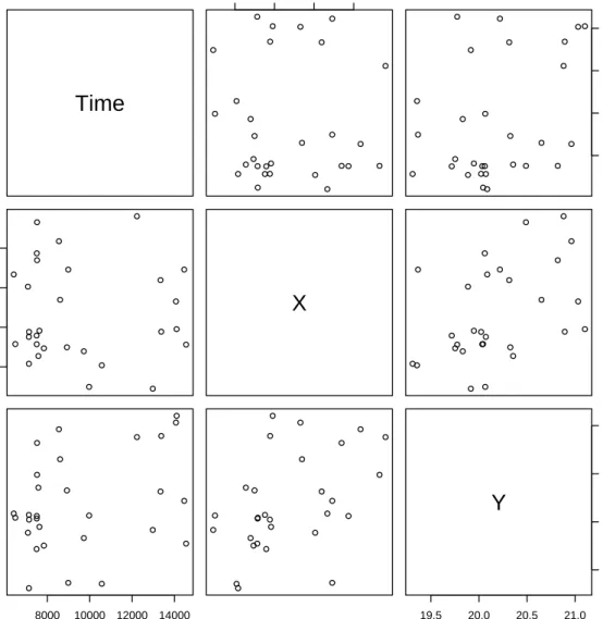
> r1 <- residuals(fit, "ordinary", m = min(ci.corners)) > pairs(r1)
Thepairs plot of the residual process is shown in Figure 2. Alternatively, we could generate approximate
thinned residuals. Here we will set the subsample sizeK equal to the number of points we obtained in the ordinary thinned residual process.
> set.seed(500)
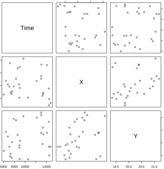
> r2 <- residuals(fit, "approx", K = nrow(r1)) > pairs(r2)
The approximate thinned residuals are shown in Figure 3. One can see from both figures that neither residual process appears to be homogeneous Poisson. Both the ordinary and approximate residuals have a clear trend from the southwest corner to the northeast corner (see the bottom middle panel) and exhibit some clustering.
Time
64.0 64.5 65.0 65.5 ● ● ● ● ● ● ● ● ●● ● ●● ● ● ● ● ● ● ● ● ● ● ● ● ● ● ● ● 8000 10000 12000 14000 ● ● ● ● ● ● ●● ●●● ● ● ● ● ● ● ● ● ● ● ● ● ● ● ● ● ● ● 64.0 64.5 65.0 65.5 ● ● ● ● ● ● ● ● ● ● ● ● ● ● ● ● ● ● ● ● ● ● ● ● ● ● ● ● ●X
● ● ● ● ● ● ● ● ● ● ● ● ● ● ● ● ● ● ● ● ● ● ● ● ● ● ● ● ● 8000 10000 12000 14000 ● ● ● ● ● ● ● ● ● ● ● ● ● ● ● ● ● ● ● ● ● ● ● ● ● ● ● ● ● ● ● ● ● ● ● ● ● ● ● ● ● ● ● ● ● ● ● ● ● ● ● ● ● ● ● ● ● ● 19.5 20.0 20.5 21.0 19.5 20.0 20.5 21.0Y
Time
64.0 64.5 65.0 65.5 ● ● ● ● ● ● ● ● ● ● ● ● ● ● ● ● ● ● ● ● ● ● ●● ● ●● ● ● 6000 8000 10000 14000 ● ● ● ● ● ● ● ● ● ● ● ● ● ● ● ● ● ● ● ● ● ● ● ● ● ● ● ● ● 64.0 64.5 65.0 65.5 ● ● ● ● ● ● ● ● ● ● ● ● ● ● ● ● ● ● ● ● ● ●● ● ● ● ● ● ●X
● ● ● ● ● ● ● ● ● ● ● ● ● ● ● ● ● ● ● ● ● ● ● ● ● ● ● ● ● 6000 8000 10000 14000 ● ● ● ● ● ● ● ● ● ● ● ● ● ● ● ● ● ● ● ● ● ● ● ● ● ● ● ● ● ● ● ● ● ● ● ● ● ● ● ● ● ● ● ● ● ● ● ● ● ● ● ● ● ● ● ● ● ● 19.5 20.0 20.5 21.0 19.5 20.0 20.5 21.0Y
While visual inspection of the residuals can be a useful tool, we may wish to conduct a more systematic test on either the ordinary or approximate thinned residuals. We will use Ripley’s K-function to test for spatial clustering and inhibition. TheK-function measures, for a given h >0, the expected proportion of points within distancehof a point in the process. The splancspackage of Rowlingson and Diggle (1993) contains an implementation of the K-function and has many other useful tools for analyzing spatial point patterns. We use the khat function insplancs to compute theK-function and theKenv.csr function to simulate confidence envelopes. For this example, we use the ordinary thinned residual process for testing purpose since it appears to have a reasonable number of points in it.
> library(splancs)
Spatial Point Pattern Analysis Code in S-Plus
Version 2 - Spatial and Space-Time analysis > b <- make.box(fit, 2:3)
> h <- seq(.1, 2, .2) > K <- khat(r1[,2:3], b, h)
> env <- Kenv.csr(nrow(r1), b, 2000, h)
Instead of plotting the rawKfunction we plot a standardized version
ˆ L(h) = s ˆ K(h) π −h
where ˆK(h) is the estimatedK function for distanceh.
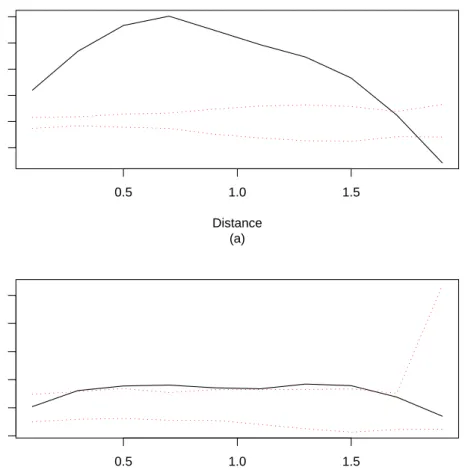
Figure 4(a-b) shows the standardizedKfunction for the original data and the ordinary thinned residuals. From Figure 4(a) it is clear that the original data are clustered. The dotted red lines are confidence envelopes for the K function produced by 2000 simulations of a homogeneous Poisson process. The standardized K
function in Figure 4(b) appears quite close to that of a homogeneous Poisson process, but the residual process still appears to be clustered. This would suggest that the model is not adequately accounting for some features in the data.
Because of the randomness involved in producing both sets of residuals, a second realization of the residual process would likely produce a different estimate of theK function. However, one strategy to deal with this could be to produce many realizations of the residual process, in turn producing many estimates of theK
function. The the range of theK function for the various residual processes can be compared to the range of theKfunction for many simulations of a homogeneous Poisson process. If the ranges overlapped closely, then that would indicate the residual process may be a close to a homogeneous Poisson process.
0.5 1.0 1.5 −0.05 0.05 0.15 Distance Standardized K function (a) 0.5 1.0 1.5 −0.2 0.2 0.6 Distance Standardized K function (b)
6.2
Fitting a One-Dimensional Cluster Model
In this section we fit a Hawkes-type cluster model to the times of the earthquake occurrences in Northern California between 1970 and 2002. The data were obtained from the Northern California Earthquake Data Center3. The dataset contains the event times of 849 earthquakes of magnitude greater that 3.0 and occurring between −121.5 and −121.0 longitude and 36.5 and 37.0 latitude. The units are in days since January 1, 1970. In this example we show two useful diagnostic plots which can be produced from the one-dimensional residual process. We also show how one might fit a sequence of models when the model can take a variable number of parameters.
The conditional intensity model we use is
λ(t) = µ+ t Z −∞ g(t−s)N(ds) = µ+X ti<t g(t−ti)
whereg is the trigger function
g(z) =
K X
k=1
akzk−1e−cz.
Here the parameter µrepresents the background rate of occurrence while the parametersa1, . . . , aK and c control the level of clustering. K represents the order of the trigger function and selecting its value is an issue we discuss below. More details about this model (and its application to earthquake data) can be found in Ogata (1988). TheRcode for this model can be found in Appendix A.
We first construct the “ptprocInit” object (settingK= 1) and then construct a penalty to ensure that the conditional intensity is positive. Here we simply restrict all of the parameters to be positive. We then fit the model withptproc.fit.
> data(cal.quakes)
> rate <- length(cal.quakes) / (365 * 33)
> pstart <- c(mu = rate, C = 1, a = 0.1)
> ppm <- ptproc(pts = cal.quakes, cond.int = hawkes.cond.int, params = pstart) > condition(ppm) <- penalty(code = NULL, condition = quote(any(params < 0)))
> fit <- ptproc.fit(ppm, optim.control = list(trace = 2), alpha = 1e+5, hessian = TRUE) > summary(fit)
Model type: HAWKES
Parameter Values: mu C a 0.05406 11.65518 2.72504 Model AIC: 5191.539 H. Pois. AIC: 6202.561 3http://quake.geo.berkeley.edu
0
2000
4000
6000
8000
10000
12000
0
2
4
6
8
Times
Conditional intensity (events / day)
Figure 5: Estimated conditional intensity function for the Hawkes model.
The parameter estimate foraindicates that immediately after an earthquake occurs, the conditional intensity is increased by about 2.7 events per day. The AIC values from the summary output show that the model does fit better than a homogeneous Poisson model. The estimated conditional intensity is shown in Figure 5. The plot was constructed by using the package functionevalCIFon a grid:
> x <- seq(0, 33*365, len = 12000) > e <- evalCIF(fit, xpts = x)
> plot(x, e, type = "l", xlab = "Times", ylab = "Conditional intensity (events / day)")
In the call toptproc.fitwe set the argumenthessian = TRUE, which directs theoptimfunction to estimate the Hessian matrix around the MLE. The estimated Hessian matrix is stored in the object returned from
ptproc.fit under the namehessian. We can compute approximate standard errors from the diagonal of
the inverse Hessian matrix. The standard errors for the parameters in this model are
mu C a
0.0022 1.8933 0.4159
A general issue with this kind of cluster model is the choice of K, the order of the polynomial in the trigger function. In the above example, we arbitrarily choseK= 1. However, we can use the AIC to compare
a number of models with different values of K. In the following example, we show how this can be done, using values ofK from 1 to 4. Note that for values ofKgreater than 2 we provide some scaling information via theparscaleargument to help the optimizer. The use of parscalewill typically be necessary to guide the optimizer towards a good solution (Venables and Ripley, 2002).
> models <- vector("list", length = 4) > for(k in 1:4) {
+ pstart <- c(mu = rate, C = rate, a = rep(.001, k))
+ ppm <- ptproc(pts = cal.quakes, cond.int = hawkes.cond.int, params = pstart)
+ condition(ppm) <- penalty(code = NULL, condition = quote(any(params < 0)))
+ parscale <- if(k < 3)
+ rep(1, k + 2)
+ else
+ pstart
+ fit <- ptproc.fit(ppm, optim.control=list(trace=3, parscale=parscale, maxit=1000),
+ alpha = 1e+5)
+ models[[k]] <- fit
+ }
> aic <- sapply(models, AIC) > names(aic) <- 1:4
> aic
1 2 3 4
5191.539 5193.541 5745.554 6042.534
It would appear thatK= 1 is the minimum AIC model of the four.
We can further examine the goodness-of-fit of theK= 1 model via residual analysis. > fit <- models[[1]]
> set.seed(900)
> r <- residuals(fit, "ordinary", m = params(fit)[1])
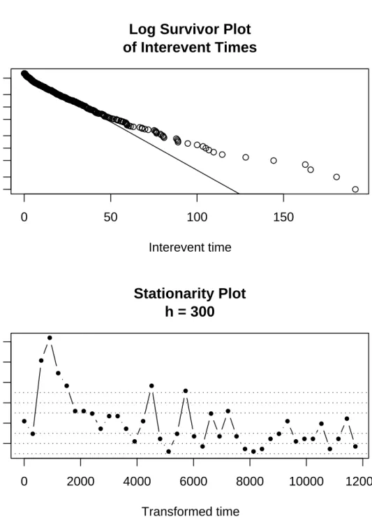
There are a number of diagnostics one can use to assess the fit of a 1-dimensional residual process. One example is a log-survivor plot of the interevent times. If the model fits well, then the residual process should be homogeneous with rate m (where m is defined in (4) and specified in the call to residuals) and the interevent times should appear as i.i.d. exponential with mean 1/m. The log-survivor plot of the interevent times of the residual process can be constructed with thelog.survfunction (included in the package) and is shown in Figure 6(a).
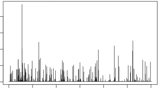
One can also check the stationarity of the residual process with thestationarityfunction. This function divides the domain into bins of a given (user-specified) length and counts the number of points falling into each bin is counted. The number of points in each bin is standardized by the theoretical mean and standard deviation and the standardized counts are plotted against the left endpoints of the bins. This plot is shown in Figure 6(b). The process generally stays within the bounds of a homogeneous Poisson process, but in one instance the count jumps far beyond three standard deviations of the expected count. This jump could indicate a region of non-stationarity in the residual process and a feature of the data which is not taken into account by the model.
● ● ● ● ●●●●●●●●●●●●●●●●●●●●●●●●●●●●●●●●●●●●●●●●●●●●●●●●●●●●●●●●●●●●●●●●●●●●●●●●●●●●●●●●●●●●●●●●●●●●●●●●●●●●●●●●●●●●●●●●●●●●●●●●●●●●●●●●●●●●●●●●●●●●●●●●●●●●●●●●●●●●●●●●●●●●●●●●●●●●●●●●●●●●●●●●●●●●●●●●●●●●●●●●●●●●●●●●●●●●●●●●●●●●●●●●●●●●●●●●●●●●●●●●●●●●●●●●●●●●●●●●●●●●●●●●●●●●●●●●●●●●●●●●●●●●●●●●●●●●●●●●●●●●●●●●●●●●●●●●●●●●●●●●●●●●●●●●●●●●●●●●●●●●●●●●●●●●●●●●●●●●●●●●●●●●●●●●●●●●●●●●●●●●●●●●●●●●●●●●●●●●●●●●●●●●●●●●●●●●●●●●●●●●●●●●●●●●●●●●●●●●●●●●●●●●●●●●●●●●●●●●●●●●●●●●●●●●●●●●●●●●●●●●●●●●●●●●●●●●●●●●●●●●●●●●●●●●●●●●●●●●●●●●●●●●●●●●●●●●●●●●●●●●●●●●●●●●●●●●●●●●●●●●●●●●●●●●●●●●●●●●●●●●●●●●●●●●●●●●●●●●●●●●●●●●●●●●●●●●●●●●●●●● ●●●●●●●●● ●●●● ● ●● ●●●● ● ● ● ● ● ●
0
50
100
150
1
5
20
100
Log Survivor Plot
of Interevent Times
Interevent time
Cumulative number
● ● ● ● ● ● ● ● ● ● ● ● ● ● ● ● ● ● ● ● ● ● ● ● ● ● ● ● ● ● ● ● ● ● ● ● ● ● ● ●0
2000
4000
6000
8000
10000
12000
−2
2
4
6
8
Stationarity Plot
h = 300
Transformed time
Standardized # of events per interval
7
Future Work
In the future we hope to develop more functions for conducting model evaluation of multi-dimensional models. We would like to add more diagnostic plots and tools to aid in residual analysis. Also, simulation based methods of model evaluation and prediction can be very useful and have not been discussed here. We hope to increase the number of simulation based tools in future releases of the package.
In addition to adding features to the ptproc package, Ritself is changing and the package will likely change withR . For example, version 1.7.0 of Rintroduced support for packages namespaces which allows package writers to export a subset of functions and hide internal functions. Also, we will eventually move to the S4 style class system (Chambers, 1998), which provides a more rigorous object oriented framework.
8
Bug Reports
Please send any bug reports or suggestions [email protected].
9
Acknowledgments
This work is part of the author’s Ph.D. dissertation from the University of California, Los Angeles. An anonymous reviewer provided many constructive comments which contributed to the revised form of this article. The author also thanks Rick Paik Schoenberg, Frauke Kreuter, and Jane Chung for useful comments on the manuscript and many interesting discussions, and James Woods for generously providing the wildfire dataset.
References
Baddeley, A. and Turner, R. (2000), “Practical Maximum Pseudolikelihood for Spatial Point Patterns,”
Australian and New Zealand Journal of Statistics, 42, 283–322.
Belisle, C. J. P. (1992), “Convergence theorems for a class of simulated annealing algorithms onRd.”Journal
of Applied Probability, 29, 885–895.
Berman, M. and Turner, T. R. (1992), “Approximating point process likelihoods with GLIM,” Applied Statistics, 41, 31–38.
Brillinger, D. R., Preisler, H. K., and Benoit, J. (2003), “Risk Assessment: A Forest Fire Example,” in
Science and Statistics, IMS, vol. 40 ofLecture Notes in Statistics.
Chambers, J. (1998),Programming with Data: A Guide to the S Language, Springer, New York.
Daley, D. J. and Vere-Jones, D. (1988),An Introduction to the Theory of Point Processes, Springer, NY. Diggle, P. J. (1983),Statistical Analysis of Spatial Point Patterns, Academic Press, NY, London.
Diggle, P. J., Chetwynd, A. G., H¨aggkvist, R., and Morris, S. E. (1995), “Second-order Analysis of Space-time Clustering,”Statistical Methods in Medical Research, 4, 124–136.
Gentleman, R. and Ihaka, R. (2000), “Lexical scope and statistical computing,” Journal of Computational and Graphical Statistics, 9, 491–508.
Harte, D. (1998), “Documentation for the Statistical Seismology Library,” Tech. Rep. 98-10, School of Mathematical and Computing Sciences, Victoria University of Wellington.
Ihaka, R. and Gentleman, R. (1996), “R: A language for data analysis and graphics,”Journal of Computa-tional and Graphical Statistics, 5, 299–314.
Lewis, P. A. W. and Shedler, G. S. (1979), “Simulation of nonhomogeneous Poisson processes by thinning,”
Naval Research Logistics Quarterly, 26, 403–413.
Nelder, J. A. and Mead, R. (1965), “A simplex algorithm for function minimization,”Computer Journal, 7, 308–313.
Nocedal, J. and Wright, S. J. (1999),Numerical Optimization, Springer.
Ogata, Y. (1978), “The asymptotic behavior of maximum likelihood estimators for stationary point pro-cesses,”Annals of the Institute of Statistical Mathematics, 30, 243–261.
— (1981), “On Lewis’ simulation method for point processes,”IEEE Transactions on Information Theory, 27, 23–31.
— (1983), “Likelihood analysis of point processes and its applications to seismological data,” Bull. Int. Statist. Inst., 50, 943–961.
— (1988), “Statistical models for earthquake occurrences and residual analysis for point processes,”Journal of the American Statistical Association, 83, 9–27.
— (1998), “Space-time point process models for earthquake occurrences,”Annals of the Institute of Statistical Mathematics, 50, 379–402.
— (1999), “Seismicity analysis through point-process modeling: a review,” Pure and Applied Geophysics, 155, 471–507.
Ogata, Y. and Tanemura, M. (1984), “Likelihood analysis of spatial point patterns,”Journal of the Royal Statistical Society, Series B, 46, 496–518.
Peng, R. D., Schoenberg, F. P., and Woods, J. (2003), “Multi-dimensional Point Process Models for Evalu-ating a Wildfire Hazard Index,” Tech. Rep. 350, UCLA Department of Statistics.
Preisler, H. K. and Weise, D. (2002), “Forest Fires Models,” in Encyclopedia of Environmetrics, eds. El-Shaarawi, A. and Piegorsch, W., Wiley, Chichester, pp. 808–810.
Rathbun, S. L. (1996), “Asymptotic properties of the maximum likelihood estimator for spatio-temporal point processes,”Journal of Statistical Planning and Inference, 51, 55–74.
Rathbun, S. L. and Cressie, N. (1994a), “Asymptotic properties of estimators for the parameters of spatial inhomogeneous Poisson point processes,”Advances in Applied Probability, 26, 122–154.
— (1994b), “A space-time survival point process for a longleaf pine forest in southern Georgia,”Journal of the American Statistical Association, 89, 1164–1174.
Ripley, B. (1976), “The second-order analysis of stationary point processes,”Journal of Applied Probability, 13, 255–266.
— (1979), “Tests of ‘randomness’ for spatial point patterns,”Journal of the Royal Statistical Society, Series B, 41, 368–374.
Rowlingson, B. and Diggle, P. (1993), “Splancs: spatial point pattern analysis code in S-Plus,” Computers and Geosciences, 19, 627–655.
Schoenberg, F. (1999), “Transforming spatial point processes into Poisson processes,”Stochastic Processes and their Applications, 81(2), 155–164.
Schoenberg, F. P. (2003), “Multi-dimensional Residual Analysis of Point Process Models for Earthquake Occurrences,” Tech. Rep. 347, UCLA Department of Statistics.
Venables, W. N. and Ripley, B. D. (2002),Modern Applied Statistics with S, Springer, NY, 4th ed.
Vere-Jones, D. (1970), “Stochastic models for earthquake occurrence,”Journal of the Royal Statistical Soci-ety, Series B, 32, 1–62.
Vere-Jones, D. and Ozaki, T. (1982), “Some examples of statistical estimation applied to earthquake data,”
A
Appendix: Code
A.1
Simple Linear Model
Below is the code for the simple linear model used in Section 6.1. The conditional intensity is of the form
λ(t, x, y) =µ+β1t+β2x+β3y.
linear.cond.int <- function(params, eval.pts, pts = NULL, data = NULL, TT = NULL) { mu <- params[1] beta <- params[-1] if(is.null(TT)) { ## Evaluate ci <- mu + eval.pts %*% beta ci <- as.vector(ci) } else { ## Integrate
total.vol <- prod(apply(TT, 2, diff)) m.vol <- sapply(1:ncol(TT), function(i)
{
z <- TT[, -i, drop=FALSE] prod(apply(z, 2, diff)) })
d <- apply(TT^2 / 2, 2, diff)
ci <- mu * total.vol + (beta * d) %*% m.vol }
ci }
A.2
Hawkes-type Cluster Model
The version of Hawkes’ self-exciting model used in Section 6.2 is
λ(t) =µ+X ti<t K X k=1 ak(t−ti)k−1e−c(t−ti).
TheRcode is as follows:
hawkes.cond.int <- function(params, eval.pts, pts = NULL, data = NULL, TT = NULL) { mu <- params[1]
C <- params[2] ak <- params[-(1:2)] K <- length(ak)
stop("K must be >= 1") if(is.null(TT)) {
S <- sapply(as.vector(eval.pts), function(x, times, ak, C) {
use <- times < x
if(!is.na(use) && any(use)) { d <- x - times[use] k <- 0:(length(ak)-1) lxk <- outer(log(d), k) + (-C * d) sum(exp(lxk) %*% ak) } else 0
}, times = as.vector(pts), ak = ak, C = C) ci <- mu + S } else { Rfunc <- function(x, L, c) { k <- 1:L g <- gamma(k) / c^k
o <- outer(x, k, pgamma, scale = 1/c) r <- o * rep(g, rep(nrow(o), ncol(o))) r } times <- as.vector(pts) ci <- mu * (TT[2,1] - TT[1,1]) S <- double(2) for(i in 1:2) {
use <- times < TT[i,1]
if(any(use)) {
r <- Rfunc(TT[i,1] - times[use], K, C) S[i] <- sum(r %*% ak)
} } ci <- ci + (S[2] - S[1]) } ci }