Alma Mater Studiorum – Universit`
a di Bologna
Dottorato di Ricerca in
Automatica e Ricerca Operativa
XXI Ciclo
MAT/09
Enhanced Mixed Integer Programming
Techniques and Routing Problems
Andrea Tramontani
Il Coordinatore I Relatori
Prof. Claudio Melchiorri Prof. Paolo Toth Prof. Andrea Lodi
Keywords
Mixed integer programming
Disjunctive cuts
Two-row cuts
Vehicle routing problems
Traveling salesman problem with time windows
Local search
Contents
Acknowledgments v
List of figures vii
List of tables x
Preface xi
1 An overview of Mixed Integer Programming 1
1.1 Introduction . . . 1
1.2 Branch-and-bound, cutting-plane and branch-and-cut . . . 2
1.3 MIP Evolution . . . 4
1.4 Main ingredients of MIP solvers . . . 6
1.4.1 Presolving . . . 7
1.4.2 Cutting plane generation . . . 8
1.4.3 Branching strategies . . . 11
1.4.4 Primal heuristics . . . 13
1.4.5 MIPping . . . 14
2 Disjunctive cuts and Gomory Mixed Integer cuts 15 2.1 Introduction . . . 15
2.2 Gomory Mixed Integer cuts . . . 15
2.3 Disjunctive cuts . . . 16
2.4 Some connections . . . 18
3 On the Separation of Disjunctive Cuts 21 3.1 Introduction . . . 21
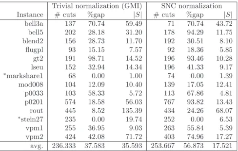
3.2 The role of normalization . . . 24
3.2.1 Why does SNC normalization work so well? . . . 27
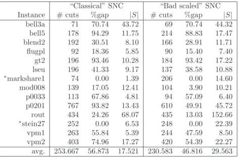
3.2.2 Nothing is perfect! . . . 28
3.2.3 Comments . . . 32
3.3 Weak CGLP rays/vertices and dominated cuts . . . 33
3.3.1 Characterization . . . 33
3.3.2 Strengthening . . . 34
3.4 Redundancy hurts . . . 38
3.4.1 Empirical Analysis . . . 41
3.4.2 Working on the Support . . . 41
3.4.3 A practical perspective . . . 43
3.5 An effective (and fast) normalization for the set covering . . . 43
3.6 Conclusions and future work . . . 48
4 Two-row cuts from the simplex tableau: a preliminary investigation 49 4.1 Introduction . . . 49
4.1.1 Multiple-row cuts . . . 49
4.1.2 Two-row cuts . . . 52
4.1.3 Lifting triangle inequalities . . . 52
4.2 A practical idea to generate triangle inequalities . . . 54
4.2.1 Strategy to generate triangles with multiple integer points on one side . . . 55
4.3 Preliminary computational results . . . 59
4.4 Open questions . . . 61
5 Integer Linear Programming Local Search for the Vehicle Routing Problem 69 5.1 Introduction . . . 69
5.2 Exponential neighborhood . . . 71
5.3 Local Search algorithm . . . 73
5.4 Node selection criteria . . . 74
5.5 Neighborhood reduction . . . 75
5.6 Neighborhood construction . . . 77
5.6.1 The column generation problem . . . 78
5.7 Computational results . . . 80
5.8 Conclusions . . . 85
6 Integer Linear Programming Local Search for the Open Vehicle Rou-ting Problem 89 6.1 Introduction . . . 89
6.2 Problem statement and literature review . . . 90
6.3 Reallocation Model . . . 91
6.3.1 Building the Reallocation Model . . . 93
6.4 Local Search Algorithm . . . 94
6.5 Computational Results . . . 95
6.6 Conclusions . . . 100
7 An extended formulation for the Traveling Salesman Problem with Time Windows 101 7.1 Introduction . . . 101
7.2 Literature review . . . 102
7.3.1 Big M Formulation (BMF) . . . 104
7.3.2 Time Indexed Formulation (TIF) . . . 104
7.3.3 Time Bucket Relaxation (TBR) . . . 106
7.3.4 Time Bucket Formulation (TBF) . . . 108
7.4 Valid inequalities for TBF . . . 109
7.4.1 Subtour elimination constraints . . . 110
7.4.2 SOP Inequalities . . . 110
7.4.3 Bucket SOPs . . . 111
7.4.4 Simple Bucket SOPs . . . 113
7.4.5 Tournament constraints . . . 114
7.4.6 Bucket tournament constraints . . . 115
7.5 Separation routines . . . 116
7.5.1 Separating bucket SOPs . . . 116
7.5.2 Separating tournament and bucket tournament constraints . . . 117
7.6 Building the formulation . . . 118
7.7 Computational results . . . 121
7.8 Conclusions . . . 125
8 Improving on Branch-and-Cut Algorithms for Generalized Minimum Spanning Trees 127 8.1 Introduction . . . 127
8.2 ILP Formulation for E-GMSTP . . . 129
8.3 ILP Formulation for L-GMSTP . . . 131
8.3.1 From L-GMSTP to E-GMSTP . . . 132
8.4 A generalization: the E/L-GMSTP . . . 133
8.5 Computational results . . . 133 8.5.1 Improving on E-GMSTP . . . 135 8.5.2 Improving on L-GMSTP . . . 138 8.5.3 E/L-GMSTP Results . . . 139 8.6 Conclusion . . . 139 Bibliography 139
Acknowledgments
First of all, my thanks go to my advisers, Andrea Lodi and Paolo Toth, strong resear-chers and tearesear-chers, for giving me the great opportunity of working with them. They followed me during all my PhD with useful suggestions, ideas and remarks. Simply, without them this work would not have been possible.
I want also to thank all the members of the Operations Research group of Bologna, for their professional help and their friendship.
Many thanks go to Matteo Fischetti, who always answers all my questions. Every day I go to Padova, I know in advance that I will learn something.
Thanks to Jon Lee, for giving me the opportunity of spending three wonderful mon-ths at IBM. And many thanks go to Sanjeeb Dash and Oktay G¨unl¨uk, real gentlemen. They followed me every day during my period at IBM and are still helping me in my research activity.
Thanks also to Santanu Dey and Laurence Wolsey, who introduced me in the two-row world.
I was honored to work with all these fantastic people and I am in debt with all of them. I really hope to have the opportunity to work with them again and again in the future.
Finally, a special thank goes to Monica. Thank you for your patience, for encou-raging and trusting me in all my choices. You are in me every day of my life and this thesis is also your thesis.
Bologna, March 15, 2009
List of Figures
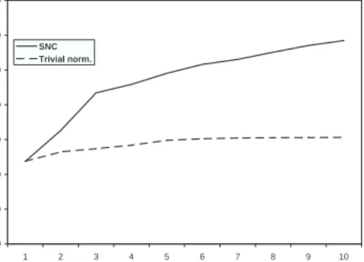
3.1 SNC vs. GMI: dual bound for instance p0201. . . 27
3.2 SNC vs. GMI: avg. cut density for instance p0201. . . 27
3.3 SNC vs. GMI: avg. cardinality of S(u, v) for instancep0201. . . 27
3.4 SNC vs. GMI: cut rank for instance p0201. . . 27
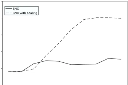
3.5 “Classical” SNC vs. “Bad scaled” SNC: dual bound for instance p0201. 30 3.6 “Classical” SNC vs. “Bad scaled” SNC: avg. cut density for instance p0201. . . 30
3.7 “Classical” SNC vs. “Bad scaled” SNC: avg. cardinality of S(u, v) for instance p0201. . . 30
3.8 “Classical” SNC vs. “Bad scaled” SNC: cut rank for instancep0201. . . 30
3.9 Example 3.1 depicted. . . 31
3.10 Example 3.2 depicted. . . 32
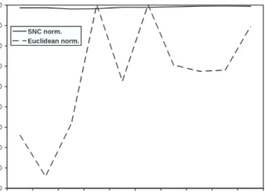
3.11 SNC vs. Euclidean normalization: dual bound for instance scpnre5. . . 46
3.12 SNC vs. Euclidean normalization: avg. cut density for instance scpnre5. 46 3.13 SNC vs. Euclidean normalization: avg. cardinality ofS(u, v) for instance scpnre5. . . 46
3.14 SNC vs. Euclidean normalization: cut rank for instance scpnre5. . . 46
4.1 Step 1(a): finding the first integer point. . . 58
4.2 Step 1(b): finding the second integer point. . . 59
4.3 Step 2: completing the triangle. . . 60
8.1 Feasible solutions for E-GMSTP. . . 128
8.2 Feasible solutions for L-GMSTP. . . 128
8.3 A graph for which E-GMSTP and L-GMSTP differ. . . 128
8.4 Example showing that Pusub⊂ Pucut. . . 131
List of Tables
1.1 Computing times for 12 Cplex versions: normalization with respect to
Cplex11.0. . . 6
1.2 Version-to-version comparison on 12Cplexversions with respect to the number of solved problems. . . 6
3.1 Trivial vs. SNC normalization. . . 26
3.2 “Classical” SNC approach vs. “Bad scaled” SNC approach. . . 29
3.3 SNC Normalization vs. SNC Normalization + CDLP. No projection (and no Balas-Jeroslow strengthening). . . 36
3.4 SNC Normalization vs. SNC Normalization + CDLP. CGLP and CDLP solved projected onto thex∗ support. Balas-Jeroslow strengthening ap-plied before and after CDLP. . . 37
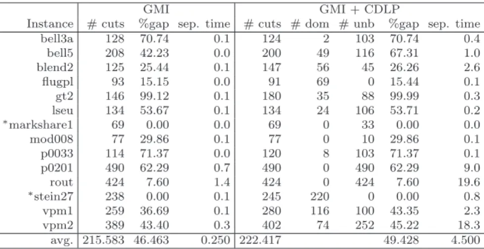
3.5 GMI vs. GMI + CDLP. CDLP solved projected onto the x∗ support. Balas-Jeroslow strengthening applied before and after CDLP. . . 37
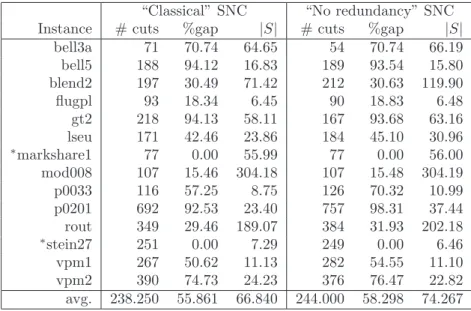
3.6 “Classical” SNC vs. “No redundancy” SNC with no projection. . . 42
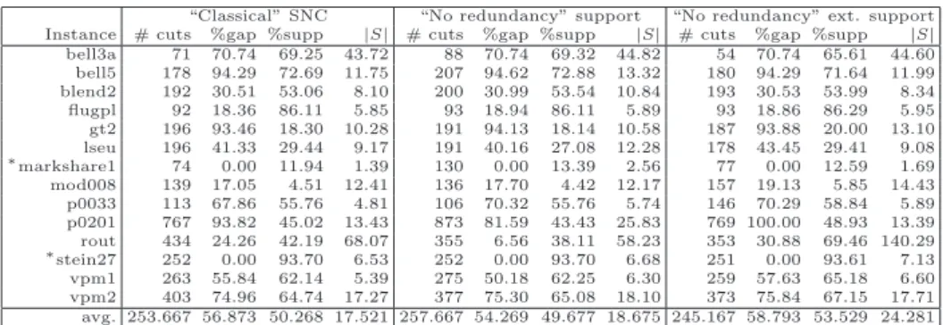
3.7 “Classical” SNC vs. “No redundancy” SNC with cuts separated projected on the support. . . 43
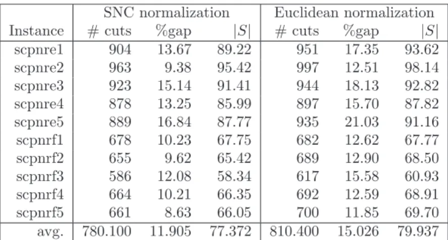
3.8 SNC normalization vs. Euclidean normalization on SCP instances. . . . 45
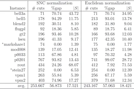
3.9 SNC normalization vs. Euclidean normalization on MIPLIB instances. . 47
3.10 SNC vs. Euclidean normalization on MIPLIB instances. Redundant constraints removed in both versions and projection on the extended support ofx∗. . . . 47
4.1 GMI cuts vs. triangle cuts: 1 round of cuts, part I. . . 62
4.2 GMI cuts vs. triangle cuts: 1 round of cuts, part II. . . 63
4.3 GMI cuts vs. triangle cuts: 1 round of cuts, part III. . . 64
4.4 GMI cuts vs. triangle cuts: 2 round of cuts, part I. . . 65
4.5 GMI cuts vs. triangle cuts: 2 round of cuts, part II. . . 66
4.6 GMI cuts vs. triangle cuts: 2 round of cuts, part III. . . 67
5.1 Computational results for the 14 CMT instances with rounded-integer costs. Initial solutions obtained by means of the C code of Toth and Vigo [167]. . . 82
5.2 Computational results for the 14 CMT instances with real costs. Initial solutions obtained by means of theC code of Toth and Vigo [167]. . . . 83
5.3 Computational results for the 20 large-scale GWKC instances. Initial
solutions obtained by means of theC code of Toth and Vigo [167]. . . . 84
5.4 Comparison on benchmark instances with “good” CVRP/DCVRP initial solutions from the literature. . . 86
6.1 Computational results on the “classical” 16 benchmark instances starting from the solutions by Fu et al. [90, 91]. . . 97
6.2 Computational results on the “classical” 16 benchmark instances starting from the best available solutions. . . 98
6.3 Computational results on the 8 large scale benchmark instances starting from the solutions by Derigs and Reuter [69]. . . 98
6.4 Current best known solution costs for the tested OVRP benchmark in-stances. . . 100
7.1 Time Bucket Formulation vs. Ascheuer et al. [11]: comparison on easy instances. . . 122
7.2 Time Bucket Formulation vs. Ascheuer et al. [11]: comparison on hard instances. . . 123
7.3 Node cuts vs. bucket cuts at the root node: comparison on hard instances.124 8.1 E-GMSTP: Euclidean Instances Comparison. . . 136
8.2 E-GMSTP: Euclidean Hard Instances Comparison. . . 136
8.3 E-GMSTP: “DHC” Instances Comparison. . . 137
8.4 L-GMSTP: “DHC” Instances Comparison. . . 140
Preface
Mixed integer programming is up today one of the most widely used techniques for dealing with hard optimization problems. On the one side, many practical optimization problems arising from real-world applications (such as, e.g., scheduling, project plan-ning, transportation, telecommunications, economics and finance, timetabling, etc) can be easily and effectively formulated as Mixed Integer linear Programs (MIPs). On the other hand, 50 and more years of intensive research has dramatically improved on the capability of the current generation of MIP solvers to tackle hard problems in practice. However, many questions are still open and not fully understood, and the mixed integer programming community is still more than active in trying to answer some of these questions. As a consequence, a huge number of papers are continuously developed and new intriguing questions arise every year.
When dealing with MIPs, we have to distinguish between two different scenarios. The first one happens when we are asked to handle a general MIP and we cannot assume any special structure for the given problem. In this case, a Linear Programming (LP) relaxation and some integrality requirements are all we have for tackling the problem, and we are “forced” to use some general purpose techniques. The second one happens when mixed integer programming is used to address a somehow structured problem. In this context, polyhedral analysis and other theoretical and practical considerations are typically exploited to devise some special purpose techniques.
Interestingly, these two different scenarios are indeed strongly related, as the gene-ral algorithmic approach used in both cases is typically the same: i.e., branch-and-cut. In particular, it is worth noting that several among the main ingredients which are actually embedded in the most effective general purpose MIP solvers (e.g., cutting pla-nes) were first devised and proven to be effective for specific combinatorial optimization problems, and only afterwards were successfully extended to the general MIP context. The history of the branch-and-cut framework itself is strongly related to the history of the Traveling Salesman Problem (TSP), probably one of the most widely studied combinatorial optimization problems. On the other side, general purpose MIP solvers are now able to solve a large variety of hard optimization problems arising from many different contexts, because most of the tools embedded in general MIP solvers (e.g., again cutting planes) are effective in practice. The connections between these two dif-ferent situations are more important every day. Having a magic black-box which allows one to solve any problem is clearly not possible, but the current trend when addressing specific problems by means of specific approaches is to keep them as much general as possible, in the spirit of possibly extend such approaches to cover other related problems.
This thesis tries to give some insights in both the above mentioned situations. The first part of the work is focused on general purpose cutting planes, which are probably the key ingredient behind the success of the current generation of MIP solvers. Chap-ter 1 presents a quick overview of the main ingredients of a branch-and-cut algorithm, while Chapter 2 recalls some results from the literature in the context of disjunctive cuts and their connections with Gomory mixed integer cuts. Chapter 3 presents a theo-retical and computational investigation of disjunctive cuts. In particular, we analyze the connections between different normalization conditions (i.e., conditions to truncate the cone associated with disjunctive cutting planes) and other crucial aspects as cut rank, cut density and cut strength. We give a theoretical characterization of weak rays of the disjunctive cone that lead to dominated cuts, and propose a practical method to possibly strengthen those cuts arising from such weak extremal solution. Further, we point out how redundant constraints can affect the quality of the generated disjunc-tive cuts, and discuss possible ways to cope with them. Finally, Chapter 4 presents some preliminary ideas in the context of multiple-row cuts. Very recently, a series of papers have brought the attention to the possibility of generating cuts using more than one row of the simplex tableau at a time. Several interesting theoretical results have been presented in this direction, often revisiting and recalling other important results discovered more than 40 years ago. However, is not clear at all how these results can be exploited in practice. As stated, the chapter is a still work-in-progress and simply presents a possible way for generating two-row cuts from the simplex tableau arising from lattice-free triangles and some preliminary computational results.
The second part of the thesis is instead focused on the heuristic and exact exploita-tion of integer programming techniques for hard combinatorial optimizaexploita-tion problems in the context of routing applications. Chapters 5 and 6 present an integer linear pro-gramming local search algorithm for Vehicle Routing Problems (VRPs). The overall procedure follows a general destroy-and-repair paradigm (i.e., the current solution is first randomly destroyed and then repaired in the attempt of finding a new improved solution) where a class of exponential neighborhoods are iteratively explored by heu-ristically solving an integer programming formulation through a general purpose MIP solver. Chapters 7 and 8 deal with exact branch-and-cut methods. Chapter 7 pre-sents an extended formulation for the Traveling Salesman Problem with Time Windows (TSPTW), a generalization of the well known TSP where each node must be visited within a given time window. The polyhedral approaches proposed for this problem in the literature typically follow the one which has been proven to be extremely effective in the classical TSP context. Here we present an overall (quite) general idea which is based on a relaxed discretization of time windows. Such an idea leads to a stronger formulation and to stronger valid inequalities which are then separated within the clas-sical branch-and-cut framework. Finally, Chapter 8 addresses the branch-and-cut in the context of Generalized Minimum Spanning Tree Problems (GMSTPs) (i.e., a class of N P-hard generalizations of the classical minimum spanning tree problem). In this chapter, we show how some basic ideas (and, in particular, the usage of general purpose cutting planes) can be useful to improve on branch-and-cut methods proposed in the literature.
Chapter 1
An overview of Mixed Integer
Programming
1.1
Introduction
A generalMixed Integer linear Program(MIP) can be defined as a “non linear” optimi-zation problem, where all the non linearities can be expressed by imposing integrality restrictions on a subset of variables: i.e., any general MIP can be expressed in the form min{cx:Ax≥b, x≥0, xj ∈Z ∀j∈J}, (1.1)
where c ∈ Rn and A ∈ Rm×n are the given objective function and constraint matrix,
while J ⊆ {1, . . . , n} denotes the set of variables constrained to be integer. When all the variables are integer-constrained (i.e., J ={1, . . . , n}), problem (1.1) is referred as apure Integer linear Program (IP).
Integer programming and mixed integer programming emerged in the late 1950’s and early 1960’s, when researchers realized that the ability to solve mixed integer program-ming models would had great impact for practical applications (see, e.g., Dantzig [63]). Up today, mixed integer programming is one of the most widely used techniques for handling hard combinatorial optimization problems. On the one side, many combinato-rial optimization problems arising from practical applications (such as, e.g., scheduling, project planning, transportation, telecommunications, economics and finance, timeta-bling) can be easily formulated as MIPs. On the other hand, several academic and commercial MIP solvers now available on the market can solve hard MIPs in practice.
The basic approach for tackling a MIP is the well knownbranch-and-boundalgorithm [110], which relies on the iterative solution of the Linear Programming (LP) relaxation of (1.1),
min{cx:Ax≥b, x≥0}, (1.2)
where all the integrality requirements on the x variables are dropped. The reason for dropping such constraints is that MIP is N P-hard while LP is polynomially solvable and general-purpose techniques for its solution are efficient in practice.
When dealing with MIPs and MIP solvers, we have to distinguish between two diffe-rent situations. The first one happens when we have no knowledge on the given problem (i.e., when we cannot assume any special structure for the given matrixAin (1.1)). In this case, we are “forced” to use a general purpose algorithmic approach which is ty-pically based on the above branch-and-bound scheme. The second one happens when the addressed formulation arises from a particular optimization problem. In this case, polyhedral analysis and other theoretical and practical considerations can be exploited to devise somespecial purpose techniques for handling the problem and/or to improve on the performance of a general purpose MIP solver. Interestingly, several among the main ingredients which are actually embedded in the most effective general purpose MIP solvers (e.g., cutting planes) were first devised and implemented for tackling spe-cific combinatorial optimization problems and spespe-cific MIP formulations. On the other hand, general purpose MIP solvers can now be easily customized in order to deal with the specific structure of MIPs arising from hard combinatorial optimization problems.
This chapter1 presents an overview of mixed integer programming techniques. In particular, Section 1.2 recalls the branch-and-bound and the branch-and-cut frameworks, Section 1.3 provides a historical overview of general purpose MIP solvers, while Section 1.4 describes some of the main ingredients of a branch-and-cut based MIP solver. The attention is focused on the current generation of general purpose MIP solvers. However, when dealing with a particular optimization problem, the main ingredients which turn out to be of crucial importance for an effective branch-and-cut algorithm are typically the same. Obviously, each one of them can be customized by exploiting the specific structure of the addressed formulation.
1.2
Branch-and-bound, cutting-plane and branch-and-cut
Roughly speaking, MIP solvers integrate the branch-and-bound and the cutting-plane
algorithms through variations of the generalbranch-and-cut scheme proposed by Pad-berg & Rinaldi [134] in the context of theTraveling Salesman Problem(TSP)2.
The branch-and-bound algorithm [110]. In its basic version the branch-and-bound algorithm iteratively partitions the solution space into sub-MIPs (the children nodes) which have the same theoretical complexity of the originating MIP (the father node, or the root node if it is the initial MIP). Given the optimal solutionx∗of the LP relaxation of the current sub-MIP (initially, the optimal solution of the LP relaxation of the root node), the branching usually creates two children by choosing one integer-constrained variable, say xj, having a fractional value x∗
j in the current x∗ solution, and imposing
thedisjunctive condition
xj ≤ bx∗jc OR xj ≥ dx∗je
1Part of this chapter has been taken from: A. Lodi, “MIP computation and beyond”, to appear in
M. J¨unger, T. Liebling, D. Naddef, W. Pulleyblank, G. Reinelt, G. Rinaldi, L. Wolsey, editors,50 Years of Integer Programming 1958–2008, Springer-Verlag, 2008 [117].
2The history of the branch-and-cut framework is tightly connected to the history of the TSP itself.
on the two created nodes (i.e., the two nodes are created by imposing, respectively, the constraintxj ≤ bx∗jc on the first one and the constraint xj ≥ dx∗je on the latter). On
each of the sub-MIPs the integrality requirement on the variables xj,∀j∈J is relaxed
and the LP relaxation is solved again. Despite the theoretical complexity, the sub-MIPs become smaller and smaller due to the partition mechanism (basically some of the deci-sions are taken) and eventually the LP relaxation is directly integral for all the variables inJ. In addition, whenever the optimal solution value cx∗ of the LP relaxation turns out to be not smaller than the best feasible solution encountered so far, called incum-bent, the node can safely be fathomed without further partitioning its corresponding sub-MIP, because none of its children will yield a better solution than the incumbent. Finally, a node is also fathomed if its LP relaxation is infeasible.
The cutting-plane algorithm [98]. Any MIP can be solved without branching by “simply” finding a linear programming description of the convex hull of its feasible solutions, i.e., a linear programming description of the set
P :=conv{x∈Rn:Ax≥b, x≥0, xj ∈Z∀j∈J}.
In order to do that, one can iteratively solve the so calledseparation problem:
(Separation problem). Given a feasible solutionx∗of the LP relaxation (1.2) which is
not feasible for the MIP (1.1), find a linear inequalityγx≥γ0 which is valid for (1.1),
i.e., satisfied by all feasible solutions ¯xof the system (1.1), while it is violated byx∗, i.e.,
γx∗< γ0.
Any inequality solving the separation problem is calledcutting plane (orcut, for short) and has the effect of tightening the LP relaxation to better approximate the convex hull.
Gomory [98] has given an algorithm that converges in a finite number of iterations for pure integer linear programs with integer data, thus implicitly proving that IPs can be solved by pure cutting-plane methods. Such an algorithm solves the separation problem above in an efficient and elegant manner in the special case in whichx∗ is an
optimal basis of the LP relaxation. No algorithm of this kind is known for MIPs, that being one of the most intriguing open questions in the area (see, e.g., Cook, Kannan & Schrijver [54]).
The and-cut algorithm incorporates the cutting-plane algorithm in the branch-and-bound scheme, by separating cuts at each3node of the search tree. The idea behind integrating the two algorithms above is that LP relaxations (1.2) do not naturally well approximate, in general, the convex hull of mixed-integer solutions of MIPs (1.1), thus some extra work to devise a better approximation by tightening any relaxation with additional linear inequalities (cutting planes) increases the chances that fewer nodes in the search tree are needed. On the other hand, pure cutting plane algorithms show, in general, a slow convergence and the addition of too many cuts can lead to very large
3Clearly, several heuristic criteria are typically used to decide, at each node of the search tree, if cut
LPs which in turn present numerical difficulties for the solvers4. As already mentioned, branch-and-cut has been initially proven to be very effective for combinatorial optimi-zation problems (like TSP, see Padberg & Rinaldi [134, 135]) with special-purpose cuts based on a polyhedral analysis of the addressed formulation. Later on, such a framework has been successfully extended to the general MIP context.
1.3
MIP Evolution
The early general-purpose MIP solvers were mainly concerned with developing a fast and reliable LP machinery used within good branch-and-bound schemes.
There are at least two remarkable exceptions to this trend. The first is a paper of Crowder, Johnson & Padberg [61] which describes the implementation of a general-purpose code for pure 0–1 IPs, called PIPX, that used the IBM linear programming system MPSX/370 and the IBM integer programming system MIP/370 as building blocks. The authors were able to solve ten instances obtained from real-world industrial applications. Those instances were very large for that time, up to 2,756 binary variables and 755 constraints. Some cutting planes were integrated in a good branch-and-bound framework (with some preprocessing to reduce variables’ coefficients) and in particular
cover inequalities which will be discussed in Section 1.4.2 below.
The second exception is a paper by Van Roy & Wolsey [170] in which the authors describe a system called MPSARX that solved mixed 0–1 industrial instances arising from applications like production planning, material requirement planning, multilevel distribution planning, etc. Also in this case, the instances were very large for the time, up to 2,800 variables and 1,500 constraints. The system acted in two phases: in phase one some preprocessing was performed and, more importantly, cutting planes were ge-nerated. Such a phase was called reformulation in [170] and performed by a system called ARX. The second phase was the solution of the new model by the mathematical programming system called SCICONIC/VM.
After the success of the two early MIP solvers [61, 170] and, mainly, the formalization of the branch-and-cut algorithm given by Padberg and Rinaldi in the TSP context [135], a major step was required to prove that cutting plane generation in conjunction with branching could work in general, i.e., without exploiting the structure of the underlying polyhedron, in particular in the cutting plane separation phase.
The proof of concept came through two papers both published in 1996. In [20], Balas, Ceria and Cornu´ejols showed that a branch-and-cut algorithm based on general-purpose disjunctive cuts (see, Balas [16]) could lead to very effective results for 0–1 MIPs. More precisely, the cutting planes used are the so called lift-and-project cuts in which the separation problem amounts to solving an LP in an extended space5.
4Note, however, that very recently Zanette, Fischetti & Balas [177] have shown that the original
cutting plane algorithm of Gomory [98] can be surprisingly effective, thus raising to many open questions related to an effective cutting planes exploitation.
The computational results in [20] showed a very competitive and stable behavior. In addition, those results showed that the quality and the speed of LP solvers in the late nineties allowed the solution of LPs as an additional building block of the overall algorithm. Such an outcome was not granted and LP rapid evolution showed to have reached a very stable state.
In [21], Balas, Ceria, Cornu´ejols and Natraj revisited the classical Gomory mixed integer cuts [99] by overruling the common sense that these cuts had a purely theore-tical interest. In fact, the results in [21] showed that, embedded in a branch-and-cut framework, Gomory mixed-integer cuts were a fundamental tool for the solution of 0–1 MIPs. Such an improvement was mainly obtained by separating and adding groups (denoted as “rounds”) of cuts6 instead of one cut at a time.
The two papers above have played a central role in the move to the current generation of MIP solvers and the fact that the use of cutting planes, and in particular within a branch-and-cut framework, has been a breakthrough is shown by the following very meaningful experiment due to Achterberg & Bixby and reported by Lodi [117]. On a testbed of 1,734 MIP instances allCplex [105] versions beginning with Cplex 1.2, the first having MIP capability, have been extensively compared. The results of this experiment are shown in Tables 1.1 and 1.2. Specifically, Table 1.1 reports the evolution of Cplexby comparing each version with the most current one, version 11.0. The first column of the table indicates the version while the second recalls the year in which the version has been released. The third and fourth columns count the number of times each version is better and worse with respect toCplex11.0, respectively: computing times within 10% are considered equivalent, i.e., counted neither better nor worse. Finally, the last column gives the computing time as geometric mean again normalized with respect to Cplex 11.0. A time limit of 30,000 CPU seconds for each instance was provided on a cluster of Intel Xeon machines 3 GHz. Besides the comparison with the current
Cplex version, the most interesting way of interpreting the results reported in the table is looking at the trend the columns show: together with a very stable decreasing of the computing time from version 1.2 up, it is clear that the biggest step forward in a version-to-version scale has been made with Cplex 6.5 which is the first having full cutting plane capability, and in particular Gomory mixed-integer cuts. Indeed, the geometric mean of the computing times drops from 21.30% to 7.47% going from version 6.0 to 6.5, by far the biggest decrease.
The trend is confirmed by the numbers reported in Table 1.2. On a slightly larger set of 1,852 MIPs (including some models in which older versions encountered numerical troubles), the table highlights the version-to-version improvement in the number of solved problems. Besides the first two columns which report the same information as Table 1.1, the third and fourth column report the number and percentage of problems solved to proven optimality, respectively. Finally, the last column gives precisely the version-to-version improvement in the percentage of problems optimally solved.
6In principle, one Gomory mixed-integer cut can be separated from each tableau row where an integer
Table 1.1: Computing times for 12 Cplex versions: normalization with respect to
Cplex11.0.
Cplex
version year better worse time 11.0 2007 – – 1.00 10.0 2005 201 650 1.91 9.0 2003 142 793 2.73 8.0 2002 117 856 3.56 7.1 2001 63 930 4.59 6.5 1999 71 997 7.47 6.0 1998 55 1060 21.30 5.0 1997 45 1069 22.57 4.0 1995 37 1089 26.29 3.0 1994 34 1107 34.63 2.1 1993 13 1137 56.16 1.2 1991 17 1132 67.90
Table 1.2: Version-to-version comparison on 12 Cplex versions with respect to the number of solved problems.
Cplex # % v-to-v %
version year optimal optimal improvement 11.0 2007 1,243 67.1% 7.8% 10.0 2005 1,099 59.3% 3.5% 9.0 2003 1,035 55.9% 2.6% 8.0 2002 987 53.3% 2.5% 7.1 2001 941 50.8% 4.3% 6.5 1999 861 46.5% 13.4% 6.0 1998 613 33.1% 1.0% 5.0 1997 595 32.1% 1.8% 4.0 1995 561 30.3% 4.4% 3.0 1994 479 25.9% 6.2% 2.1 1993 365 19.7% 4.7% 1.2 1991 278 15.0% —
1.4
Main ingredients of MIP solvers
This section provides an overview of the main ingredients of a branch-and-cut based MIP solver. For many more details on the arguments of this section we refer the reader to Part II of the PhD dissertation of Achterberg [3].
1.4.1 Presolving
In the presolving (often called preprocessing) phase the solver tries to detect certain changes in the input that will probably lead to a better performance of the solution process. This is done without changing the set of optimal solutions of the problem at hand and it affects two main situations.
On the one side, it is often the case that MIP models, in particular those originating from real-world applications and created by using modeling languages, contain some “garbage”, i.e., irrelevant or redundant information that tend to slow down the solution process forcing the solver to perform useless operations. More precisely, there are two types of sources of inefficiency: first, the models are unnecessary large and thus harder to manage. This is the case in which there are redundant constraints or variables which are already fixed and nevertheless appear in the model as additional constraints. Second, the variable bounds can be unnecessary large or the constraints could have been written in a loose way, for example with coefficients weaker than they could possibly be.
Thus, modern MIP solvers have the capability of “cleaning up” the models so as to create a presolved instance associated with the original one on which the MIP technology is then applied. With respect to the two issues above, MIP presolve is able to reduce the size of the problems by removing such redundancies and it generally provides tools that, exploiting the information on the integrality of the variables in set J, strengthen variables’ bound and constraints’ coefficients. If the first improvement has only the effect of making each LP relaxation smaller and then quicker to be solved, the second one has the, sometimes crucial, effect of making such relaxations stronger, i.e., better approximating the convex hull of mixed-integer solutions.
On the other hand, more sophisticated presolve mechanisms are also able to discover important implications and sub-structures that might be of fundamental importance later on in the computation for both branching purposes and cutting plane generation. As an example, the presolve phase determines the clique table or conflict graph, i.e., groups of binary variables such that no more than one can be non-zero at the same time. The conflict graph is then fundamental to separateclique inequalities (see, Johnson and Padberg [107]) which are written as
X
j∈Q
xj ≤1 (1.3)
where Q denotes a subset of (indices of) binary variables with the property, stated above, that at most one of them can be non-zero.
The most fundamental work about presolving is the one of Savelsbergh [157] to which the interested reader is referred to.
At first glance, the presolving phase seems to be relevant only when dealing with “badly-written” MIP formulations, which typically contain many redundancies and weak constraints. However, this is definitely not the case, as experienced with the
Traveling Salesman Problem with Time Windows (TSPTW) (see Chapter 7). For this problem, a strong MIP formulation is proposed and a branch-and-cut algorithm is inve-stigated in this thesis. In this context, aspecial-purposepreprocessing which exploits the
specific structure of the problem turns out to be of crucial importance for all the above mentioned reasons. First, it is fundamental for reducing the size of the formulation and for strengthening the corresponding LP relaxation. Second, it allows to discover important connections among the variables which are then used to derive strong valid inequalities, separated during the branch-and-cut algorithm. We refer the reader to Chapter 7 for a detailed account on this work.
1.4.2 Cutting plane generation
As shown in Section 1.3, cutting plane generation has been a key step for the success of MIP solvers and their capability of being effective for a wide variety of problems. Several groups of cuts are actually available in most academic and commercial MIP solvers (as, e.g., Cbc [44], Cplex [105] and Xpress [65]). These groups are strongly related each other, and include Chv´atal-Gomory cuts [98, 49], Gomory mixed-integer cuts [99], mixed-integer rounding cuts [129, 67], {0,12} cuts [41], lift-and-project cuts [16, 20] and split cuts [54] (also known as disjunctive cuts). Essentially, all these inequalities are obtained by applying a disjunctive argument on a mixed-integer set of a single constraint only, which is often derived by aggregating many others. Gomory mixed-integer cuts and disjunctive cuts are addressed more in detail in Chapter 2 of this thesis. For a brilliant and unified presentation of all these family of cuts we refer the reader to Cornu´ejols [57].
Besides the groups above and clique inequalities already discussed in the previous section, two more classes of very useful cuts are generally used within a MIP solver, namelycover inequalities and flow cover inequalities, which are briefly discussed in the following.
Cover cuts. Somehow similarly to the clique inequalities, cover constraints define a property on a set of binary variables. More precisely, given a knapsack kind constraint in the form γx ≤ γ0 where we assume that γ ∈ Z+|V|, γ0 ∈ Z+ and V is a subset of (indices of) binary variables, a set Q⊆V is called acover ifPj∈Qγj > γ0. The cover is said to be minimal if Pj∈Q\{`}γj ≤ γ0 for all `∈ Q. In other words, Q is a set of binary variables which cannot be all together non-zero at the same time. In the light of the definition above, the simplest version of a cover inequality is
X
j∈Q
xj ≤ |Q| −1. (1.4)
The amount of work devoted to cover cuts is huge starting with the seminal work of Balas [15] and Wolsey [174]. In particular, cover cuts do not define facets, i.e., poly-hedral faces of dimension one less of the dimension of the associated polyhedron7, but can be lifted (see, Padberg [133]) to become facet defining.
Flow cover cuts. The polyhedral investigation of the so called0–1 single node flow problem is at the base of the definition of flow cover cuts by Padberg, Van Roy & Wolsey
7For a detailed presentation of polyhedral basic concepts as dimensions, faces, facets, etc. the reader
[136]. Essentially, this is a fixed charge problem with arcs incoming and outgoing to a single node: to each of these arcs is associated a continuous variables measuring the flow on the arc and upper bounded by the arc capacity, if the flow over the arc is non-zero a fixed cost must be paid and this is triggered by a binary variable associated with the same arc. A flow balance on the node must also be satisfied. Flow cover cuts can then be devised as mixed-integer rounding inequalities (see, Marchand [122]) and then strengthened by lifting (see, Gu, Nemhauser & Savelsbergh [101]). We also refer the to Louveaux & Wolsey [118] for a general discussion on these mixed-integer sets.
It is worth noting that despite the origin of the flow cover cuts is a specific poly-hedral context, they are useful and applied in general within MIP solvers. The reason is that it is easy to aggregate variables (and constraints) of a MIP in order to derive a mixed-integer set like the 0–1 single node flow set (see, e.g., [122]).
The separation of all mentioned cuts (including cliques) but lift-and-project cuts is N P-hard for a general x∗. Note that this is not in contrast with the fact that one can separate, e.g., Gomory mixed-integer cuts by a polynomial (very cheap) procedure [98, 99] once the fractional solution x∗ to be cut off is a vertex of the continuous
rela-xation.
Cutting planes have been widely studied in the literature and the arsenal of sepa-ration algorithms has been continuously enlarged over the years. However, there are still several fundamental questions about the use of cutting planes which are probably not fully answered, thus reducing what we could really gain from cuts. Some of these questions are discussed in the following and are probably strongly related each other.
Accuracy. Accuracy checks are needed in basically all parts of a MIP solver but maybe the most crucial part is cutting plane generation. Sophisticated cutting plane procedures challenge the floating-point arithmetic of the solvers heavily, the danger being the generation of invalid cuts, i.e., linear inequalities cutting off mixed-integer feasible solutions, eventually the optimal one. The common reaction is defining confi-dence threshold values for a cut to be safe. This is only a heuristic action, probably very conservative too. The accuracy issue has been recently investigated in two papers. Margot [123] studied a methodology for testing accuracy and strength of cut generators based on random dives of the search tree by recording a well-chosen set of indicators. Cook, Dash, Fukasawa & Goycoolea [53] proposed a method that slightly weakens the Gomory mixed-integer cuts but makes them “safe” with respect to accumulation of floating-point errors.
Both papers above investigate the accuracy issue of cutting plane generation mainly from a research viewpoint. At the moment, the standard method of dealing with inac-curacy of cuts in the solvers is discarding “suspicious” or “dangerous” cuts without doing extra work to either test their correctness or separating them in a proven careful way. Among other indicators, cutting planes with high rank8 are considered suspicious
8The rank of the inequalities in the original formulation is 0 while every inequality obtained as
in the sense that they might have accumulated relevant floating-point errors while dense inequalities are said to be dangerous since they generally slow down the LP machinery.
Cut selection and interaction. The number of existing procedures for generating cuts is relevant and that is the number of cuts we could generate at any round. Thus, one of the most relevant issues is which cuts should be selected and added to the current LP relaxation. In other words, cuts should be able to interact in a profitable way together so as to have an overall “cooperative behavior”. Results in this direction have been reported by Andreello, Caprara & Fischetti [8].
Cut strength. The strength of a cut is generally measured by its violation. However, scaling, normalization conditions and other factors can make such a measure highly misleading. If this is the case, cut selection is very hard and, for example, separating over a larger class of cuts is not necessarily a good idea with respect to preferring a smaller (thus, theoretically weaker) sub-class which is known to produce effective cuts in practice. An example of such a counter-intuitive behavior is the separation of Chv´atal-Gomory cuts instead of their stronger mixed integer rounding version as experienced by Dash, G¨unl¨uk & Lodi [67]: separating over the sub-class as a heuristic mixed inte-ger rounding procedure helped accelerating the cutting plane convergence dramatically9. The role of the rank and other aspects such as normalization conditions, (i.e., con-ditions to truncate the cone associated with disjunctive cutting planes) are not fully understood and much more can be done in this direction. Some new results on the connections among normalization conditions, cut rank, cut density and cut strength are presented in Chapter 3 of this thesis and also appear in Fischetti, Lodi & Tramontani [85].
We close this section by mentioning one of the most exciting and potentially helpful challenges in the cutting plane context. A recent series of papers [7, 29, 39, 60, 71, 75, 176] has brought the attention of the community to the possibility of generating cuts using more than one row of the simplex tableau at a time. Thesemultiple-row cutsare based on the characterization of lattice-free triangles (and lattice-free bodies in general) instead of simply split disjunctions as in the case of the single row tableau cuts discussed in this section. Some new ideas for generating two-row cuts from the simplex tableau by exploiting lattice-free triangles and some computational results in this direction are presented in Chapter 4 of this thesis.
be obtained as combination of two or more rows of rank≤k−1 but not as a combination of inequalities of rank≤k−2 only. The reader is referred to Chv´atal [49] for a more formal definition of the rank of an inequality and its implications for IP.
9Note that such an outcome might be also related to the stable behavior of Chv´atal-Gomory cuts
with respect to Gomory mixed-integer or mixed integer rounding cuts due to their numerical accuracy [83].
1.4.3 Branching strategies
The branching mechanism introduced in Section 1.1 requires to take two independent and important decisions at any step: node selection and variable selection. We will analyze them separately in the following by putting more attention on the latter.
Node Selection. One extreme is the so calledbest-bound first strategy in which one always considers the most promising node, i.e., the one with the smallest LP value, while the other extreme isdepth first where one goes deeper and deeper in the tree and starts backtracking only once a node is fathomed, i.e., it is either mixed-integer feasible, or LP infeasible or it has a dual bound not better (smaller) than the incumbent. The main advantages and drawbacks of each strategy are well known: the former explores less nodes but generally maintains a larger tree in terms of memory while the latter can explode in terms of nodes and it can, in the case some bad decisions are taken at the beginning, explore useless portions of the tree itself. All other techniques, more or less sophisticated, are basically hybrids around these two ideas, like interleaving best-bound and diving10 in an appropriate way.
Variable Selection. The variable selection problem is the one of deciding how to partition the current node, i.e., on which variable one has to branch on in order to create the two children. For a long time, a classical choice has been branching on the most fractional variable, i.e., in the 0–1 case the closest to 0.5. That rule has been computationally shown by Achterberg, Koch & Martin [5] to be worse than a com-plete random choice. However, it is of course very easy to evaluate. In order to devise stronger criteria one has to do much more work. The extreme is the so called strong branching technique (see, e.g., Applegate, Bixby, Chv´atal & Cook [9] and Linderoth & Savelsbergh [116]). In its full version, at any node one has to tentatively branch on each candidate fractional variable and select the one on which the increase in the bound on the left branch times the one on the right branch is the maximum. Of course, this is generally unpractical but its computational effort can be easily limited in two ways: on the one side, one can define a much smaller candidate set of variables to branch on and, on the other hand, can limit to a fixed (small) amount the number of Simplex pivots to be performed in the variable evaluation. Another sophisticated technique is
pseudocost branching which goes back to Benichou, Gauthier, Girodet & Hentges [31] and keeps a history of the success (in terms of the change in the LP relaxation value) of the branchings already performed on each variable as an indication of the quality of the variable itself. The most recent effective and sophisticated method is called reliability branching [5] and it integrates strong and pseudocost branchings. The idea is to define a reliability threshold, i.e., a level below which the information of the pseudocosts is not considered accurate enough and some strong branching is performed. Such a threshold is mainly associated with the number of previous branching decisions that involved the variable.
More sophisticated branching mechanisms are clearly possible, an example being
the so called Special Order Sets (SOS) branching (Beale & Tomlin [30]). When, for instance, the formulation at hand contains a constraint of the form
X
j∈B
xj = 1,
whereB is a set of binary variables, one can branch by imposing the disjunctive
condi-tion X j∈B1 xj = 1 OR X j∈B2 xj = 1
on the children nodes, withB1∪B2 =B and B1∩B2 =∅. This idea is detailed, e.g., in Williams [173].
Karamanov & Cornu´ejols [108] highlighted the possibility of using some cutting plane theory in the branching context. They experimented with branching on Gomory mixed-integer disjunctions obtained by the optimal basis of the LP relaxation. More precisely, from each tableau rowiin which an integer variablex`is basic at the fractional
value x∗
`, say ¯aix = x∗`, instead of deriving the associated Gomory mixed-integer cut,
they consider the corresponding disjunction
πx≤ bx∗`c OR πx≥ dx∗`e, where πj = b¯aijc ifj∈J, j 6=`, ¯aij− b¯aijc ≤x∗ `− bx∗`c d¯aije ifj∈J, j 6=`, a¯ij− b¯aijc> x∗`− bx∗`c 1 ifj=` 0 otherwise.
The best disjunction according to a heuristic measure is selected for branching.
In the line of the work in [108], Cornu´ejols, Liberti & Nannicini [59] try to improve the disjunction to be used for branching by row manipulations in the spirit of the reduce-and-split approach for cuts [6].
Branching on general disjunctions has been also used in context less related to cut-ting plane theory. A pioneering work in this direction is the one of Owen & Mehrotra [132] where the general disjunctions to branch on are generated by a search heuristic in the neighborhood containing all disjunctions with coefficients in {−1,0,1} on the integer variables with fractional values at the current node. Moreover, branching on appropriate disjunctions has recently been proposed in the context of highly symmetric MIPs by Ostrowsky, Linderoth, Rossi & Smriglio [131]. Finally, Bertacco [33] has expe-rimented with branching on general disjunctions either associated with “thin” directions of the polyhedron or resulting in the maximization of the corresponding lower bound. A very similar approach has been followed recently by Mahajan & Ralphs [121].
As discussed above, until now the methods proposed in research papers and imple-mented by MIP solvers to do enumeration have been rather structured, very relying on the tree paradigm which has proven to be stable and effective. Few attempts of seriously revisiting the tree framework have been made, one notable exception being
the work of Chv´atal called resolution search [50]. In that paper, the idea is to detect conflicts, i.e., sequences of variable fixings that yield an infeasible subproblem, making each sequence minimal and use the information to construct an enumeration strategy. A similar concept of conflicts has been used by Achterberg [2, 3] to do propagation in MIP and it has been known in the Artificial Intelligence and SATisfiability (SAT) com-munities with the name of “no good recording” (see, e.g., Stallman & Sussman [159]) since the seventies.
1.4.4 Primal heuristics
Primal heuristics, going from easy to complex, are generally used within any effective branch-and-cut algorithm. These heuristics typically start from the fractional solution of the continuous relaxation of each sub-MIP of the search tree, trying to produce a feasible mixed-integer solution. In the last years, the continuous hybridization between rounding and diving techniques with local search has dramatically improved the capability of the current generation of MIP solvers to quickly find in the search tree very high quality solutions.
Following the structure of Chapter 9 of [3], we distinguish among the following types of heuristics.
Rounding heuristics. Starting from a feasible solution of the continuous relaxation (generally the optimal one) one rounds up or down the fractional values of the variables inJ by trying to produce a mixed-integer solution still satisfying the linear constraints. This can be done in a straightforward and very fast manner or in a more and more complex way, i.e., by allowing some backtracking mechanism in the case a (partial) mixed-integer assignment becomes infeasible.
Diving heuristics. With respect to a rounding heuristic, the diving is performed in an iterative way: after rounding one or more variables the LP relaxation is solved again and the process is iterated. In this category, Achterberg [3] distinguishes between “hard” rounding in which the variables are really fixed to a specified value and “soft” rounding in which the effect is obtained implicitly by changing the objective function coefficient of the variables to be “rounded” in an appropriate way. In the latter ca-tegory falls the feasibility pump heuristic [81, 34, 4]. The idea of the algorithm is to alternatively satisfy either the linear constraints (by solving LP relaxations) or integer constraints (by applying rounding). The LP relaxations are obtained by replacing the original objective function with one taking into account the distance with respect to the current mixed-integer rounded solution. If the trajectory of the rounded solutions intersects the one of the LP (neighborhood) relaxations, then a feasible solution with respect to both the linear constraints and the integer ones has been found. Such an algorithmic framework has been recently extended to convex mixed-integer non-linear programming [38].
Improving heuristics. The heuristics in this category are designed to improve the quality of the current incumbent solution, i.e., they exploit that solution or a group of
solutions so as to get a better one. These heuristics are usually local search methods and we have recently seen a variety of algorithms which solve sub-MIPs for exploring the neighborhood of the incumbent or of a set of solutions. When these sub-MIPs are solved in a general-purpose fashion, i.e., through a nested call to a MIP solver, this is referred to as MIPping [82] and will be the content of Section 1.4.5 below. Improvement heuristics of this type have connections to the so called metaheuristic techniques [95] which have proven very successful on hard and large combinatorial problems in the ni-neties. Techniques from metaheuristics have been now incorporated in the MIP solvers, see e.g., [82, 152]. As a result, MIP solvers have now improved their ability of quickly finding very good feasible solutions and can be seen as competitive heuristic techniques if used in a truncated way, i.e., with either a time or node limit.
It is interesting to note that Achterberg [3] has shown that the impact of heuristics is not dramatic in terms of ability of the MIP solver to prove optimality in a (much) quicker way. However, in many cases mixed integer programming techniques are used to derive effective heuristics for hard optimization problems. In this context, the goal is to find high-quality feasible solutions, with a minor attention to the possibility of also prove the optimality. Clearly, when the MIP solver is embedded in an overall heuristic procedure, the capability of the solver itself to produce high-quality feasible solutions very quickly is of crucial importance to improve on the performance of the overall algorithm.
1.4.5 MIPping
The MIP computation has reached such an effective and stable quality to allow the solution of sub-MIPs during the solution of a MIP itself, i.e., the MIPping approach [84]. In other words, optimization sub-problems are formulated as general-purpose MIPs and solved, often heuristically, by using MIP solvers, i.e., without taking advantage of any special structure. The novelty is not in solving optimization sub-problems having different levels of complexity, but in using a general-purpose MIP solver for handling them. In some sense such a technique, originally proposed by Fischetti & Lodi [82] for modeling large neighborhoods of 0–1 solutions, shows the high quality of the current generation of MIP solvers like the solution of large LPs in the cutting plane generation phase [20] showed more than ten years ago the effectiveness of the LP phase.
After the original paper on the primal heuristic side, the MIPping technique has been successfully applied in the cutting plane generation phase [83], for accelerating Benders decomposition [148], and again to devise very high quality primal solutions [62], just to cite a few applications.
In Chapters 5 and 6 of this thesis, the MIPping approach is investigated to derive an effective local search algorithm in the context of the Vehicle Routing Problem(VRP). The overall local search algorithm is based on a class of exponential neighborhoods which are iteratively explored, in a heuristic way, by solving an IP through a general purpose MIP solver. The results of Chapters 5 and 6 also appear, respectively, in Toth & Tramontani [169] and Salari, Toth & Tramontani [153].
Chapter 2
Disjunctive cuts and Gomory
Mixed Integer cuts
2.1
Introduction
Disjunctive cuts for mixed integer linear programs have been introduced by Egon Balas [16] in the late 70’s, and successfully exploited in practice since the late 90’s (see, e.g., Balas, Ceria and Cornu´ejols [20]). This chapter recalls some theoretical results from the literature related to the separation ofdisjunctive cuts, and the main connections between disjunctive cuts and Gomory Mixed Integer (GMI) cuts [99]. A new investigation and some new results on this topic are developed in Chapter 3.
In the following we consider a mixed integer set S of the form S = {x ∈ Rn :
Ax≥ b, x ≥0, xj ∈ Z ∀j ∈J}, where A ∈Rm×n is the given constraint matrix and
J ⊆ {1, . . . , n}denotes the set of variables constrained to be integer. We assume for the sake of simplicity the set S to be nonempty and we denote with P ={x ∈Rn :Ax≥
b, x≥0} the underlying polyhedron obtained by dropping all the integral requirements from S.
2.2
Gomory Mixed Integer cuts
Let αx ≥ α0 be any valid inequality for P (recall that, by Farkas lemma, the valid inequalities forP are of the form (λA+µ)x≥λb−δ, withλ∈Rm
+,µ∈Rn+,δ ∈R+), and add a nonnegative surplus variablestoαx≥α0, thus obtaining the valid equality αx−s=α0. Define f0=α0− bα0c,fj =αj− bαjcfor anyj ∈J, and assumef0 >0. Then, the following equality is valid forP,
X j∈J:fj≤f0 fjxj+ X j∈J:fj>f0 (fj−1)xj+ X j6∈J αjxj −s=k+f0,
wherek is some integer. Sincek≤ −1 or k≥0, any x∈S satisfies the disjunction
X j∈J:fj≤f0 −fj 1−f0xj + X j∈J:fj>f0 1−fj 1−f0xj+ X j6∈J −αj 1−f0xj+ s 1−f0 ≥1
OR X j∈J:fj≤f0 fj f0xj+ X j∈J:fj>f0 fj−1 f0 xj+ X j6∈J αj f0xj − s f0 ≥1.
The above disjunction is of the form a1z ≥ 1 or a2z ≥ 1 which naturally implies
P
jmax{a1j, a2j}zj ≥1 for anyz≥0. For eachj, one of the coefficient in the disjunction
is positive and the other is negative. Hence, the following inequality is valid forS:
X j∈J:fj≤f0 fj f0xj+ X j∈J:fj>f0 1−fj 1−f0xj+ X j6∈J:αj>0 αj f0xj+ X j6∈J:αj<0 −αj 1−f0xj+ s 1−f0 ≥1. (2.1)
The inequality (2.1) is the well knownGomory Mixed Integerinequality [99]. Clearly, the GMI (2.1) can be expressed in the x space by rewriting the surplus variable s in terms of the x variables (i.e., by rewriting s=αx−α0). TheGMI closure is obtained from P by adding all the GMI inequalities forS.
As shown by Caprara and Letchford [42] and, independently, by Cornu´ejols and Li [58], it is N P-hard to optimize a linear function over the GMI closure relative to a polyhedronP. Equivalently, given a point ¯x∈P\S, it isN P-hard to find a GMI which separates ¯x or show that none exists. Note, however, that this is not in contrast with the problem of finding a GMI cut that cuts off a basic solutionx∗ of the polyhedronP.
Indeed, given a basic solution x∗ of P and its corresponding tableau, each row of the tableau corresponding to a basic variablexj, withj ∈J and x∗j fractional, can be used
to derive a violated GMI cut by following the simple procedure described above.
2.3
Disjunctive cuts
For any given disjunction of the form
πx≤π0 OR πx≥π0+ 1 (2.2)
such that (π, π0) ∈ Zn+1, π
j = 0 ∀j 6∈ J, let P0 (respectively, P1) be the polyhedron obtained from P by imposing the additional restriction πx≤ π0 (resp., πx ≥π0+ 1). A disjunctive inequality is an inequality γx ≥ γ0 valid both for P0 and P1, and then also forconv(P0∪P1) and hence forconv(S). Disjunctive cuts which can be derived by imposing a single disjunction such as (2.2) on a polyhedron P are also known assplit cuts; see Cook, Kannan, and Schrijver [54]. The intersection of all split inequalities (for all the possible disjunctions of the form (2.2)) is called thesplit closurerelative toP.
By Farkas lemma, the validity ofγx≥γ0 forP0and forP1can always be certified by means of nonnegative multipliers (u, u0, v, v0) associated with the inequalities defining P0 and P1 according to the following scheme:
P0 (u) Ax ≥ b (u0) −πx ≥ −π0 P1 (v) Ax ≥ b (v0) πx ≥ π0+ 1
Given a fractional solutionx∗ ofP, a most-violated disjunctive cut can therefore be found by solving the following problem that determines the disjunction (π, π0) and the Farkas multipliers so as to maximize the violation of the resulting cut with respect to the given pointx∗:
min γx∗−γ 0 γ ≥uA−u0π γ ≥vA+v0π γ0 ≤ub−u0π0 γ0 ≤vb+v0(π0+ 1) u, v, u0, v0≥0 π0∈Z πj ∈Z, j∈J πj = 0, j6∈J. (2.3)
By construction, any feasible solution with negative objective function value in (2.3) corresponds to a violated disjunctive cut. However, when solving the separation pro-blem (2.3), there are two different aspects to be considered. On the one side, (2.3) is a mixed integer nonlinear program involving products of integer and continuous variables. On the other hand, even if the disjunction is fixed a priori, the resulting Linear Program (LP) is defined on a cone and needs to be truncated so as to produce a bounded LP in case a violated cut exists. From a theoretical point of view, Caprara and Letchford [42] have formulated the problem of optimizing over the split closure as a mixed integer nonlinear program and have shown that the separation problem for split cuts is stron-gly N P-hard. On a practical side, Balas and Saxena [26] addressed the problem by exploiting the normalization condition u0 +v0 = 1, which allows one to restate (2.3) and to solve it as a parametric MIP with a single parameter. A similar approach was also proposed by Dash, G¨unl¨uk and Lodi [66, 67] in the context of the Mixed Integer Rounding (MIR) closure1.
A typical approach for separating disjunctive cuts in a branch-and-cut framework is the one arising from Balas, Ceria and Cornu´ejols [20], which showed the effectiveness of
lift-and-projectcuts in the context of 0–1 MIPs2. This approach can be easily extended to general MIPs (i.e., MIPs with general integer-constrained variables) and can be de-scribed as follows. Given the current fractional solutionx∗ of the current LP relaxation,
a violated disjunction of the form (2.2) is fixed, withπx∗−π
0 ∈ ]0,1[, and a disjunctive cut is separated by solving the so-called Cut Generating Linear Program (CGLP):
(CGLP) min γx∗−γ 0 γ ≥uA−u0π γ ≥vA+v0π γ0≤ub−u0π0 γ0≤vb+v0(π0+ 1) u, v, u0, v0 ≥0. (2.4)
1Note that the MIR closure and the Split closure define the same polyhedron; see e.g., [57, 66, 67]. 2Lift-and-project cuts are a particular class of disjunctive cuts for 0–1 MIPs arising from elementary
As already stated, CGLP is defined on a cone and needs to be truncated with a sui-table normalization condition so as to produce a bounded LP in case a violated cut exists. Different normalization conditions lead in general to very different results. The connections among normalization conditions, cut strength and other related issues are investigated in Chapter 3 of this thesis.
Usually, the CGLP is projected onto the support of x∗ (see, e.g., [20]). Given a
variable xk such that x∗k = 0, the value of the cut coefficient γk does not affect the
cut violation. Hence, one can avoid considering the CGLP constraints associated with γk. The resulting (reduced) CGLP is then solved and the cut coefficient γk is derived afterwards as
γk= max{uAk−u0πk, vAk+v0πk}, (2.5)
where all the Farkas multipliers are fixed as in the optimal solution of the reduced CGLP.
In practice, the disjunction selected for solving CGLP is typically elementary, i.e., it involves only one integer variable, thus reading xj ≤ bx∗jc ORxj ≤ dx∗je (j ∈J). As
such, the disjunctive cut only exploits the integrality requirement on a single variable and can therefore be easily improved by ana posteriori cut strengthening procedure as the one proposed by Balas and Jeroslow [23].
Theorem 2.1 (Balas and Jeroslow [23]). Let (γ, γ0, u, v, u0, v0) be an optimal solution of CGLP with respect to a certain disjunction (π, π0). Define mj = uAuj−0+vAv0j, and
˜ γj =
½
min{uAj −u0bmjc, vAj+v0dmje} if j∈J,
max{uAj, vAj} if j6∈J.
Then the inequality ˜γx≥ γ0 is valid for conv(S) and dominates γx≥ γ0 over the set
{x∈Rn:x≥0}.
The strengthening described in the above theorem can be interpreted as finding the best disjunction for the given set of multipliers, by fixingπj =bmjc or πj =dmje for any j∈J.
2.4
Some connections
GMI cuts and disjunctive cuts are strongly related. On the one side, Nemhauser and Wolsey [128, 129] have shown that the GMI closure and the split closure relative to a polyhedronP are identical. On the other hand, Balas and Perregaard [24, 25] discovered several connections between GMIs from the tableau and basic solutions of CGLP in the context of 0–1 MIPs3.
In particular, Balas and Perregaard [25] addressed the CGLP truncated with nor-malization m X i=1 ui+ m X i=1 vi+u0+v0= 1
3All the results from [24, 25] were presented in the context of 0–1 MIPs. The results reported in this