University of California, Berkeley
U.C. Berkeley Division of Biostatistics Working Paper Series
Year
Paper
Multiple Testing Procedures: R multtest
Package and Applications to Genomics
Katherine S. Pollard
∗Sandrine Dudoit
†Mark J. van der Laan
‡∗Center for Biomolecular Science and Engineering, University of California, Santa Cruz, [email protected]
†Division of Biostatistics, School of Public Health, University of California, Berkeley, [email protected]
‡Division of Biostatistics, School of Public Health, University of California, Berkeley, [email protected]
This working paper is hosted by The Berkeley Electronic Press (bepress) and may not be commer-cially reproduced without the permission of the copyright holder.
http://biostats.bepress.com/ucbbiostat/paper164 Copyright c2004 by the authors.
Multiple Testing Procedures: R multtest
Package and Applications to Genomics
Katherine S. Pollard, Sandrine Dudoit, and Mark J. van der Laan
Abstract
The Bioconductor R package multtest implements widely applicable
resampling-based single-step and stepwise multiple testing procedures (MTP) for controlling
a broad class of Type I error rates, in testing problems involving general data
gen-erating distributions (with arbitrary dependence structures among variables), null
hypotheses, and test statistics. The current version of multtest provides MTPs for
tests concerning means, differences in means, and regression parameters in linear
and Cox proportional hazards models. Procedures are provided to control Type
I error rates defined as tail probabilities for arbitrary functions of the numbers of
false positives and rejected hypotheses. These error rates include tail probabilities
for the number of false positives (generalized family-wise error rate, gFWER) and
the proportion of false positives among the rejected hypotheses (TPPFP).
Single-step and Single-step-down common-cut-off (maxT) and common-quantile (minP)
proce-dures, that take into account the joint distribution of the test statistics, are proposed
to control the family-wise error rate (FWER), or chance of at least one Type I
er-ror. In addition, augmentation multiple testing procedures are provided to control
the gFWER and TPPFP, based on any initial FWER-controlling procedure. The
results of a multiple testing procedure can be summarized using rejection regions
for the test statistics, confidence regions for the parameters of interest, or adjusted
p-values. A key ingredient of our proposed MTPs is the test statistics null
distri-bution (and estimator thereof) used to derive rejection regions and corresponding
confidence regions and adjusted p-values. Both bootstrap and permutation
esti-mators of the test statistics null distribution are available. The S4 class/method
object-oriented programming approach was adopted to summarize the results of a
MTP. The modular design of multtest allows interested users to readily extend the
package’s functionality. Typical testing scenarios are illustrated by applying
vari-ous MTPs implemented in multtest to the Acute Lymphoblastic Leukemia (ALL)
dataset of Chiaretti et al. (2004), with the aim of identifying genes whose
ex-pression measures are associated with (possibly censored) biological and clinical
outcomes.
Note.This document is an expanded version of a chapter to be published in the monographBioinformatics and Computational Biology Solutions Using R and Bioconductor[Gentleman et al., 2005]. The reader is referred to this book for a discussion of other relevant packages developed as part of the Bioconductor project.
0.1
Introduction
0.1.1
Motivation
Current statistical inference problems in biomedical and genomic data anal-ysis routinely involve the simultaneous test of thousands, or even millions, of null hypotheses. Examples include:
• identification of differentially expressed genes in microarray exper-iments, i.e., genes whose expression measures are associated with possibly censored responses or covariates;
• tests of association between gene expression measures and Gene Ontology (GO) annotation;
• identification of transcription factor binding sites in ChIP-Chip experiments [Kele¸s et al., 2004];
• genetic mapping of complex traits using single nucleotide polymor-phisms (SNP).
The above testing problems share the following general characteristics: • inference for high-dimensional multivariate distributions, with
com-plex and unknown dependence structures among variables;
• broad range of parameters of interest, such as, regression coefficients and correlations;
• many null hypotheses, in the thousands or even millions; • complex dependence structures among test statistics.
Motivated by these applications, we have developed and implemented (in R and SAS) resampling-based single-step and stepwise multiple testing pro-cedures (MTP) for controlling a broad class of Type I error rates, in testing problems involving general data generating distributions (with arbitrary dependence structures among variables), null hypotheses (defined in terms of submodels for the data generating distribution), and test statistics (e.g., t-statistics,F-statistics). The different components of our multiple testing methodology are treated in detail in a collection of related articles [Pollard and van der Laan, 2004, Dudoit et al., 2004, van der Laan et al., 2004,,
ii
Dudoit et al., 2004] and a book in preparation [Dudoit and van der Laan, 2004].
The early article of Pollard and van der Laan [2004] and subsequent ar-ticle of Dudoit et al. [2004] establish a general statistical framework for multiple hypothesis testing. A key feature of the proposed MTPs is the
test statistics null distribution(rather than data generating null distribu-tion) used to derive rejection regions (i.e., cut-offs) for the test statistics and resulting confidence regions and adjusted p-values. For Type I error rates defined as arbitrary parameters θ(FVn) of the distribution of the
number of Type I errors Vn (e.g., the generalized family-wise error rate,
gF W ER(k) =P r(Vn> k), or chance of at least (k+1) false positives), this
null distribution is the asymptotic distribution of the vector of null value shifted and scaled test statistics. Resampling procedures (e.g., based on the non-parametric or model-based bootstrap) are proposed to conveniently obtain consistent estimators of the null distribution and the correspond-ing test statistic cut-offs and adjustedp-values [Pollard and van der Laan, 2004, Dudoit et al., 2004, van der Laan et al., 2004, Dudoit and van der Laan, 2004].
Pollard and van der Laan [2004] and Dudoit et al. [2004] also derive
single-step common-cut-off and common-quantile proceduresfor controlling general Type I error rates of the formθ(FVn).
van der Laan et al. [2004] focus on control of the family-wise error rate,F W ER = gF W ER(0), and provide step-down common-cut-off and common-quantile procedures, based on maxima of test statistics (maxT) and minima of unadjustedp-values (minP), respectively. van der Laan et al. [2004], and subsequently Dudoit et al. [2004] and Dudoit and van der Laan [2004], propose general classes ofaugmentation multiple testing procedures
(AMTP), obtained by adding suitably chosen null hypotheses to the set of null hypotheses already rejected by an initial MTP. In particular, given
any FWER-controlling procedure, they show how one can trivially ob-tain augmentation procedures controlling tail probabilities for the number (gFWER) and proportion (TPPFP) of false positives among the rejected hypotheses. The results of a simulation study comparing augmentation pro-cedures to existing gFWER- and TPPFP-controlling MTPs are reported in Dudoit et al. [2004]. Finally, the multiple testing methodology and appli-cations to genomic data analysis are the subject of a book in preparation for Springer [Dudoit and van der Laan, 2004].
In order to make this general methodology broadly and readily accessible to the biomedical and genomic data analysis community, we have imple-mented the above MTPs in the Bioconductor R packagemulttest, which is the subject of the present paper.
0.1.2
Outline
The Bioconductor R package multtest provides software implementations of the multiple testing procedures mentioned in Section 0.1.1 and discussed in greater detail in Section 0.2. Specifically, given a multivariate dataset and user-supplied choices for the test statistics, Type I error rate and its target level(s), estimator of the test statistics null distribution, and proce-dure for deriving rejection regions, the main user-level functionMTPreturns unadjusted and adjustedp-values, cut-off vectors for the test statistics, and estimates and confidence regions for the parameters of interest. Both boot-strap and permutation estimators of the test statistics null distribution are available and can optionally be output to the user. The S4 class/method object-oriented programming approach was adopted to represent the re-sults of a MTP. Several methods are defined to produce numerical and graphical summaries of these results. A modular programming approach, which uses function closures, allows interested users to readily extend the package’s functionality, by inserting functions for new test statistics and testing procedures.
The present paper is organized as follows. Section 0.2 provides a sum-mary of our proposed multiple testing procedures. Section 0.3 discusses their software implementation in the Bioconductor R package multtest. Section 0.4 describes applications of the MTPs to the Acute Lymphoblas-tic Leukemia (ALL) dataset of Chiaretti et al. [2004], with the aim of identifying genes whose expression measures are associated with (possibly censored) biological and clinical outcomes such as: tumor cellular subtype (B-cell vs. T-cell), tumor molecular subtype (BCR/ABL, NEG, ALL1/AF4, E2A/PBX1, p15/p16, NUP-98), and time to relapse. Finally, Section 0.5 discusses ongoing efforts.
0.2
Multiple hypothesis testing methodology
0.2.1
Multiple hypothesis testing framework
Hypothesis testingis concerned with using observed data to test hypotheses, i.e., make decisions, regarding properties of the unknown data generating distribution. For example, microarray experiments might be conducted on a sample of patients in order to identify genes whose expression levels are associated with survival. Below, we discuss in turn the main ingredients of a multiple testing problem. These include data, null and alternative hy-potheses, test statistics, multiple testing procedure, Type I and Type II errors, adjustedp-values, test statistics null distribution, rejection regions. Further detail on each of these components can be found in Dudoit et al. [2004] and Dudoit and van der Laan [2004]; specific proposals of MTPs are
iv
given in Sections 0.2.4 – 0.2.6.
Software implementation.Themulttest package is designed so that the main components of a MTP are specified as arguments to the package’s primary user-level function, MTP: the data via the arguments X, W, Y, Z,
Z.incl, and Z.test; the test statistics via test, robust, standardize,
alternative, andpsi0; the Type I error rate viatypeoneandalpha(and
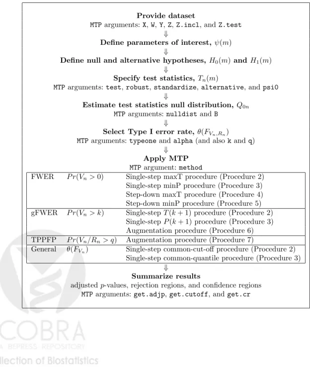
also the error rate-specific parameterskandq); the test statistics null dis-tribution vianulldistandB; and the MTP itself viamethod. The desired output, i.e., adjustedp-values, rejection regions, and confidence regions, are specified using the argumentsget.adjp,get.cutoff, andget.cr, respec-tively. The main steps in applying a multiple testing procedure are listed in the flowchart of Table 1 and typical testing scenarios are illustrated in Section 0.4, using the ALL dataset of Chiaretti et al. [2004] as a case study.
Data. Let X1, . . . , Xn be a random sampleof n independent and
identi-cally distributed (i.i.d.) random variables, X ∼ P ∈ M, where the data generating distributionP is an element of a particularstatistical modelM (i.e., a set of possibly non-parametric distributions). In a microarray exper-iment, for example,X is a vector of gene expression measurements, which we observe for each ofnarrays.
Null and alternative hypotheses. In order to cover a broad class of testing problems, defineM null hypotheses in terms of a collection of sub-models, M(m)⊆ M, m = 1, . . . , M, for the data generating distribution P. The M null hypotheses are defined as H0(m)≡I(P ∈ M(m)) and the
correspondingalternative hypothesesas H1(m)≡I(P /∈ M(m)). In many
testing problems, the submodels concernparameters, i.e., functions of the data generating distribution P, Ψ(P) = ψ = (ψ(m) : m = 1, . . . , M), such as means, differences in means, correlation coefficients, and regression parameters. For instance, the full modelMmight refer to the set of all con-tinuousM–variate distributions and the submodel M(m), corresponding to themth null hypothesis, might be the subset ofM for which the mth component of the mean vector ψ = E[X] is non-negative, i.e., M(m) = {P ∈ M : ψ(m) ≥ 0} (further parametric restrictions, such as normal-ity, may be imposed on the models). One distinguishes between two types of testing problems: one-sided tests, where H0(m) = I(ψ(m) ≤ ψ0(m)),
andtwo-sided tests, whereH0(m) = I(ψ(m) =ψ0(m)). The user-supplied
hypothesizednull values,ψ0(m), are frequently zero.
Let H0 = H0(P) ≡ {m : H0(m) = 1} = {m : P ∈ M(m)} be the
set ofh0 ≡ |H0|true null hypotheses, where we note that H0 depends on
the data generating distribution P. Let H1 = H1(P) ≡ Hc0(P) = {m :
H1(m) = 1}={m :P /∈ M(m)} be the set of h1 ≡ |H1|=M −h0 false
is to accurately estimate the set H0, and thus its complement H1, while
controlling probabilistically the number of false positives.
Test statistics. A testing procedure is a data-driven rule for deciding whether or not torejecteach of theM null hypothesesH0(m), i.e., declare
thatH0(m) is false (zero) and henceP /∈ M(m). The decisions to reject or
not the null hypotheses are based on anM–vector oftest statistics,Tn =
(Tn(m) :m= 1, . . . , M), that are functionsTn(m) =T(X1, . . . , Xn)(m) of
the data,X1, . . . , Xn. Denote the typically unknown (finite sample) joint
distributionof the test statisticsTn byQn=Qn(P).
Single-parameter null hypotheses are commonly tested usingt-statistics, i.e., standardized differences,
Tn(m)≡
Estimator−Null value Standard error =
√
nψn(m)−ψ0(m)
σn(m)
. (1)
In general, theM–vectorψn= (ψn(m) :m= 1, . . . , M) denotes an
asymp-totically linear estimator of the parameter M–vector ψ = (ψ(m) : m =
1, . . . , M) and (σn(m)/
√
n : m = 1, . . . , M) denote consistent estimators
of the standard errors of the components of ψn. For tests of means, one
recovers the usual one-sample and two-sample t-statistics, where ψn(m)
andσn(m) are based on empirical means and variances, respectively (e.g.,
two-samplet-statistic in Equation (3), p. vi, for the ALL microarray data analysis of Section 0.4). In some settings, it may be appropriate to use (un-standardized)difference statistics, Tn(m)≡
√
n(ψn(m)−ψ0(m)) [Pollard
and van der Laan, 2004]. Test statistics for other types of null hypotheses includeF-statistics,χ2-statistics, and likelihood ratio statistics.
Multiple testing procedure.A multiple testing procedure (MTP) pro-vides rejection regions, Cn(m), i.e., sets of values for each test statistic
Tn(m) that lead to the decision to reject the null hypothesis H0(m). In
other words, a MTP produces a random (i.e., data-dependent) subsetRn
of rejected hypotheses that estimatesH1, the set of true positives,
Rn=R(Tn, Q0n, α)≡ {m:H0(m) is rejected}={m:Tn(m)∈ Cn(m)},
(2) whereCn(m) = C(Tn, Q0n, α)(m),m= 1, . . . , M, denote possibly random
rejection regions. The long notation R(Tn, Q0n, α) and C(Tn, Q0n, α)(m)
emphasizes that the MTP depends on: (i) thedata,X1, . . . , Xn, through the
M–vector oftest statistics,Tn= (Tn(m) :m= 1, . . . , M); (ii) a (estimated)
test statisticsnull distribution,Q0n, for deriving rejection regions for each
Tn(m) and the resulting adjusted p-values (Section 0.2.2); and (iii) the
nominal levelα, i.e., the desired upper bound for a suitably defined Type I error rate.
Unless specified otherwise, it is assumed that large values of the test statistic Tn(m) provide evidence against the corresponding null
hypoth-vi
esis H0(m), that is, we consider rejection regions of the form Cn(m) =
(cn(m),∞), where cn(m) are to-be-determined critical values, or cut-offs,
computed under the null distributionQ0nfor the test statisticsTn (Section
0.2.2).
Example.Suppose that, as in the analysis of the ALL dataset of Chiaretti et al. [2004] (Section 0.4), one is interested in identifying genes that are differentially expressed in two populations of ALL cancer patients, those with the B-cell subtype and those with the T-cell subtype. The data con-sist of randomJ–vectorsX, where the firstM entries ofX are microarray expression measures onM genes of interest and the last entry,X(J), is an indicator for the ALL subtype (1 for B-cell, 0 for T-cell). Then, the param-eter of interest is anM–vector of differences in mean expression measures in the two populations,ψ(m) =E[X(m)|X(J) = 1]−E[X(m)|X(J) = 0],
m= 1, . . . , M. To identify genes with higher mean expression measures in
the B-cell compared to T-cell ALL subjects, one can test the one-sided null hypotheses H0(m) = I(ψ(m) ≤ 0) vs. the alternative hypotheses
H1(m) = I(ψ(m)>0), using two-sample Welcht-statistics
Tn(m)≡ ¯ X1,n1(m)−X¯0,n0(m) q n−01(m)σ2 0,n0(m) +n −1 1 (m)σ12,n1(m) , (3) where nk(m), ¯Xk,nk(m), and σ 2
k,nk(m) denote, respectively, the sample
sizes, sample means, and sample variances, for patients with tumor sub-typek,k = 0,1. The null hypotheses are rejected, i.e., the corresponding genes are declared differentially expressed, for large values of the test statis-ticsTn(m).
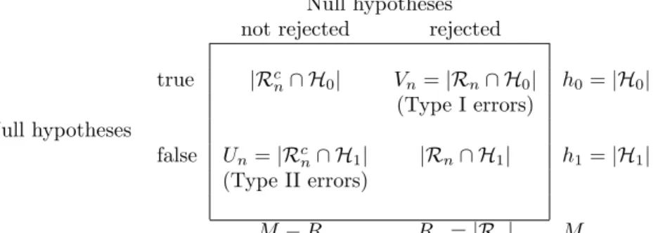
Type I and Type II errors.In any testing situation, two types of errors can be committed: afalse positive, orType I error, is committed by rejecting a true null hypothesis, and afalse negative, orType II error, is committed when the test procedure fails to reject a false null hypothesis. The situation can be summarized by Table 2, below, where the number of Type I errors isVn≡ |Rn∩ H0|=Pm∈H0I(Tn(m)∈ Cn(m)) and the number of Type II
errors isUn ≡ |Rcn∩ H1|=Pm∈H1I(Tn(m)∈ C/ n(m)).
Note that both Un and Vn depend on the unknown data generating
distribution P through the unknown set of true null hypotheses H0 =
H0(P). The numbersh0=|H0|and h1=|H1|=M−h0of true and false
null hypotheses areunknown parameters, the number of rejected hypotheses
Rn ≡ |Rn|= P
M
m=1I(Tn(m) ∈ Cn(m)) is an observable random variable,
and the entries in the body of the table,Un,h1−Un,Vn, andh0−Vn, are
unobservable random variables(depending onP throughH0(P)).
Ideally, one would like to simultaneously minimize both the number of Type I errors and the number of Type II errors. Unfortunately, this is not feasible and one seeks atrade-offbetween the two types of errors. A
stan-dard approach is to specify an acceptable levelαfor the Type I error rate and derive testing procedures, i.e., rejection regions, that aim to minimize the Type II error rate, i.e., maximizepower, within the class of procedures with Type I error rate at mostα.
Type I error rates.When testing multiple hypotheses, there are many possible definitions for the Type I error rate and power of a test proce-dure. Accordingly, we adopt the general framework proposed in Dudoit et al. [2004] and Dudoit and van der Laan [2004], and define Type I error rates asparameters,θn=θ(FVn,Rn), of the joint distributionFVn,Rn of the
numbers of Type I errorsVn and rejected hypothesesRn. Such a general
representation covers the following commonly-used Type I error rates.
Generalized family-wise error rate (gFWER), or probability of at least (k+ 1) Type I errors,k= 0, . . . ,(h0−1),
gF W ER(k)≡P r(Vn> k) = 1−FVn(k), (4)
whereFVnis the discrete cumulative distribution function (c.d.f.) on
{0, . . . , M} for the number of Type I errors, Vn. When k = 0, the
gFWER is the usual family-wise error rate (FWER), or probability of at least one Type I error,
F W ER≡P r(Vn>0) = 1−FVn(0). (5)
The FWER is controlled, in particular, by the classical Bonferroni procedure.
Per-comparison error rate (PCER), or expected value of the proportion of Type I errors among theM tests,
P CER≡ 1 ME[Vn] = 1 M Z vdFVn(v). (6)
Tail probabilities for the proportion of false positives(TPPFP) among the rejected hypotheses,
T P P F P(q)≡P r(Vn/Rn> q) = 1−FVn/Rn(q), q∈(0,1), (7)
whereFVn/Rnis the c.d.f. for the proportionVn/Rn of false positives
among the rejected hypotheses, with the convention thatVn/Rn ≡0
ifRn= 0.
False discovery rate(FDR), or expected value of the proportion of false positives among the rejected hypotheses,
F DR≡E[Vn/Rn] =
Z
qdFVn/Rn(q), (8)
again with the convention thatVn/Rn≡0 ifRn= 0 [Benjamini and
viii
Note that while the gFWER is a parameter of only themarginal distri-butionFVn of the number of Type I errorsVn (tail probability, or survivor
function, for Vn), the TPPFP is a parameter of the joint distribution of
(Vn, Rn) (tail probability, or survivor function, forVn/Rn).
Error rates based on theproportionof false positives (e.g., TPPFP and FDR) are especially appealing for large-scale testing problems such as those encountered in genomics, compared to error rates based on thenumberof false positives (e.g., gFWER), as they do not increase exponentially with the number of tested hypotheses.
The aforementioned error rates are part of the broad class of Type I er-ror rates considered in Dudoit et al. [2004] and Dudoit and van der Laan [2004], and defined as tail probabilities P r(g(Vn, Rn) > q) and expected
valuesE[g(Vn, Rn)] for an arbitrary function g(Vn, Rn) of the numbers of
false positivesVn and rejected hypothesesRn. The gFWER and TPPFP
correspond to the special cases g(Vn, Rn) = Vn and g(Vn, Rn) = Vn/Rn,
respectively.
Adjusted p-values. The notion of p-value extends directly to multiple testing problems, as follows. Given a MTP Rn(α) = R(Tn, Q0n, α), the
adjusted p-value Pe0n(m) = Pe(Tn, Q0n)(m), for null hypothesis H0(m), is
defined as the smallest Type I error level α at which one would reject H0(m), that is,
e
P0n(m) ≡ inf{α∈[0,1] :m∈ Rn(α)} (9)
= inf{α∈[0,1] :Tn(m)∈ Cn(m)}, m= 1, . . . , M.
Note that unadjusted or marginal p-values, for the test of a single hy-pothesis, correspond to the special case M = 1. For a continuous null distributionQ0n, the unadjustedp-value for null hypothesisH0(m) is given
byP0n(m) =P(Tn(m), Q0n,m) = ¯Q0n,m(Tn(m)), where Q0n,mand ¯Q0n,m
denote, respectively, the marginal c.d.f.’s and survivor functions for Q0n.
For example, the adjustedp-values for the classical Bonferroni procedure for FWER control are given byPe0n(m) = min(M P0n(m),1).
As in single hypothesis tests, the smaller the adjusted p-value, the stronger the evidence against the corresponding null hypothesis. IfRn(α)
is right-continuous at α, in the sense that limα0↓αRn(α0) = Rn(α), then
one has two equivalent representations for the MTP, in terms of rejection regions for the test statistics and in terms of adjustedp-values,
Rn(α) ={m:Tn(m)∈ Cn(m)}={m:Pe0n(m)≤α}. (10)
Reporting the results of a MTP in terms of adjusted p-values, as op-posed to the binary decisions to reject or not the hypotheses, offers several advantages. (i) Adjustedp-values can be defined forany Type I error rate
evi-dence against each null hypothesis in terms of the Type I error rate for the
entire MTP. (iii) They areflexible summariesof a MTP, in that results are supplied forall levelsα, i.e., the levelαneed not be chosen ahead of time. (iv) Finally, adjustedp-values provide convenient benchmarks to compare
different MTPs, whereby smaller adjustedp-values indicate a less conser-vative procedure.
Confidence regions.For the test of single-parameter null hypotheses and for any Type I error rate of the formθ(FVn), Pollard and van der Laan [2004]
and Dudoit and van der Laan [2004] provide results on the correspondence between single-step MTPs andθ–specific confidence regions.
0.2.2
Test statistics null distribution
One of the main tasks in specifying a MTP is to derive rejection regions for the test statistics such that the Type I error rate is controlled at a desired level α, i.e., such that θ(FVn,Rn) ≤ α, for finite sample control,
or lim supnθ(FVn,Rn)≤ α, for asymptotic control. It is common practice,
especially for FWER control, to setα= 0.05. However, one is immediately faced with the problem that thetrue distributionQn =Qn(P) of the test
statisticsTn is usuallyunknown, and hence, so are the distributions of the
numbers of Type I errors, Vn = Pm∈H0I(Tn(m)∈ Cn(m)), and rejected
hypotheses,Rn =P M
m=1I(Tn(m)∈ Cn(m)). In practice, the test statistics
true distributionQn(P) is replaced by a null distributionQ0 (or estimate
thereof, Q0n), in order to derive rejection regions and resulting adjusted
p-values.
The choice of null distributionQ0is crucial, in order to ensure that (finite
sample or asymptotic) control of the Type I error rate under theassumed
null distribution Q0 does indeed provide the required control under the
truedistributionQn(P). For proper control, the null distributionQ0 must
be such that the Type I error rate under this assumed null distribution
dominatesthe Type I error rate under the true distribution Qn(P). That
is, one must have θ(FVn,Rn) ≤ θ(FV0,R0), for finite sample control, and
lim supnθ(FVn,Rn)≤ θ(FV0,R0), for asymptotic control, whereV0 and R0
denote, respectively, the numbers of Type I errors and rejected hypotheses under the assumed null distributionQ0.
For error rates θ(FVn) (e.g., gFWER), defined as arbitrary parameters of
the distribution of the number of Type I errors Vn, we propose as null
distribution the asymptotic distributionQ0 =Q0(P) of the M–vectorZn
of null value shifted and scaled test statistics [Pollard and van der Laan, 2004, Dudoit et al., 2004, van der Laan et al., 2004, Dudoit and van der
x Laan, 2004], Zn(m)≡ s min 1, τ0(m) V ar[Tn(m)] Tn(m) +λ0(m)−E[Tn(m)] . (11)
For the test of single-parameter null hypotheses usingt-statistics, the null values are λ0(m) = 0 and τ0(m) = 1. For testing the equality of K
population means using F-statistics, the null values are λ0(m) = 1 and
τ0(m) = 2/(K−1), under the assumption of equal variances in the
differ-ent populations. By shifting the test statisticsTn(m) as in Equation (11),
one obtains a sequence of random variablesZn(m) that are asymptotically
stochastically greater than the test statisticsTn(m) for the true null
hy-potheses. Thus, the number of Type I errorsV0under the null distribution
Q0, is asymptotically stochastically greater than the number of Type I
er-rorsVn under the true distributionQn=Qn(P). Dudoit et al. [2004] and
van der Laan et al. [2004] prove that the null distributionQ0 does indeed
provide the desired asymptotic control of the Type I error rate θ(FVn),
for general data generating distributions (with arbitrary dependence struc-tures among variables), null hypotheses (defined in terms of submodels for the data generating distribution), and test statistics (e.g., t-statistics, F-statistics).
For a broad class of testing problems, such as the test of single-parameter null hypotheses usingt-statistics as in Equation (1), the null distributionQ0
is anM–variate Gaussian distribution with mean vector zero and covariance matrix Σ∗(P):Q0 =Q0(P)≡N(0,Σ∗(P)). For tests of means, where the
parameter of interest is the M–dimensional mean vector Ψ(P) = ψ = E[X], the estimator ψn is simply the M–vector of sample averages and
Σ∗(P) is the correlation matrix ofX ∼P,Cor[X]. More generally, for an asymptotically linear estimatorψn, Σ∗(P) is the correlation matrix of the
vector influence curve (IC).
Note that the following important points distinguish our approach from existing approaches to Type I error rate control. Firstly, we are only con-cerned with Type I error control under thetrue data generating distribution
P. The notions of weak and strong control (and associated subset pivotal-ity, Westfall & Young [Westfall and Young, 1993], p. 42–43) are therefore irrelevant to our approach. Secondly, we propose a null distribution for the test statistics, Tn ∼ Q0, and not a data generating null distribution,
X ∼ P0 ∈ ∩Mm=1M(m). The latter practice does not necessarily provide
proper Type I error control, as the test statistics’assumednull distribution Qn(P0) and theirtrue distributionQn(P) may have different dependence
structures, in the limit, for the true null hypothesesH0.
Procedure 1 Bootstrap estimation of the null distribution Q0
1. LetP?
n denote an estimator of the data generating distributionP. For
thenon-parametric bootstrap,P?
Pn, that is, samples of sizenare drawn at random, with replacement
from the observed data, X1, . . . , Xn. For the model-based bootstrap,
P?
n is based on a model M for the data generating distribution P,
such as the family of M–variate Gaussian distributions.
2. Generate B bootstrap samples, each consisting of ni.i.d. realizations of a random variable X#∼P?
n.
3. For the bth bootstrap sample,b= 1, . . . , B, compute anM–vector of test statistics, Tn#(·, b) = (Tn#(m, b) : m= 1, . . . , M). Arrange these
bootstrap statistics in an M ×B matrix, T#n = Tn#(m, b)
, with rows corresponding to the M null hypotheses and columns to the B
bootstrap samples.
4. Compute row means,E[Tn#(m,·)], and row variances,V ar[Tn#(m,·)],
of the matrixT#n, to yield estimates of the true meansE[Tn(m)]and
variances V ar[Tn(m)]of the test statistics, respectively.
5. Obtain an M ×B matrix, Z#
n = Zn#(m, b)
, of null value shifted and scaled bootstrap statistics Z#
n(m, b), by row-shifting and scaling
the matrix T#
n as in Equation 11 using the bootstrap estimates of
E[Tn(m)] and V ar[Tn(m)] and the user-supplied null values λ0(m)
andτ0(m). That is, compute
Zn#(m, b) ≡ s min 1, τ0(m) V ar[Tn#(m,·)] (12) ×Tn#(m, b) +λ0(m)−E[Tn#(m,·)] .
6. The bootstrap estimateQ0nof the null distributionQ0is the empirical
distribution of theB columnsZ#
n(·, b)of matrix Z#n.
In practice, since the data generating distributionPis unknown, then so is the proposed null distributionQ0=Q0(P). Resampling procedures, such
as the bootstrap procedure of section 1, may be used to conveniently obtain consistent estimatorsQ0nof the null distributionQ0and of the
correspond-ing test statistic cut-offs and adjustedp-values [Pollard and van der Laan, 2004, Dudoit et al., 2004, van der Laan et al., 2004, Dudoit and van der Laan, 2004]. This bootstrap procedure is implemented in the internal
func-tionboot.resampleand may be specified via the argumentsnulldistand
Bof the main user-level functionMTP. The reader is referred to our earlier articles and book in preparation for further detail on the choice of test statisticsTn, null distribution Q0, and approaches for estimating this null
distribution. Accordingly, we take the test statisticsTn and their null
dis-tribution Q0 (or estimate thereof, Q0n) as given, and denote the set and
number of rejected hypotheses by Rn(α) = R(Tn, Q0n, α) andRn(α) (or
the shorterRn and Rn), respectively, to emphasize only the dependence
xii
0.2.3
Rejection regions
Having selected a suitable test statistics null distribution, there remains the main task of specifying rejection regions for each null hypothesis, i.e., cut-offs for each test statistic. Among the different approaches for defining rejection regions, we distinguish between the following.
Common-cut-off vs. common-quantile multiple testing proce-dures. In common-cut-off procedures, the same cut-off c0 is used
for each test statistic (cf. FWER-controlling maxT procedures [sec-tions 2 and 4], based on maxima of test statistics). In contrast, in
common-quantile procedures, the cut-offs are theδ0–quantiles of the
marginal null distributions of the test statistics (cf. FWER-controlling minP procedures [sections 3 and 5], based on minima of unadjusted p-values). The latter procedures tend to be more “balanced” than the former, as the transformation top-values places the null hypotheses on an equal footing. However, this comes at the expense of increased computational complexity.
Single-step vs. stepwise multiple testing procedures.Insingle-step procedures, each null hypothesis is evaluated using a rejection region that is independent of the results of the tests of other hypotheses. Improvement in power, while preserving Type I error rate control, may be achieved bystepwise procedures, in which rejection of a par-ticular null hypothesis depends on the outcome of the tests of other hypotheses. That is, the (single-step) test procedure is applied to a sequence of successively smaller nested random (i.e., data-dependent) subsets of null hypotheses, defined by the ordering of the test statistics (common-cut-off MTPs) or unadjusted p-values (common-quantile MTPs). In step-down procedures, the hypotheses corresponding to themost significanttest statistics (i.e., largest absolute test statistics or smallest unadjustedp-values) are considered successively, with fur-ther tests depending on the outcome of earlier ones. As soon as one fails to reject a null hypothesis, no further hypotheses are rejected. In contrast, forstep-up procedures, the hypotheses corresponding to the
least significanttest statistics are considered successively, again with further tests depending on the outcome of earlier ones. As soon as one hypothesis is rejected, all remaining more significant hypotheses are rejected.
Marginal vs. joint multiple testing procedures. Marginal multiple testing procedures are based solely on the marginal distributions of the test statistics, i.e., on cut-off rules for individual test statistics or their corresponding unadjustedp-values (e.g., classical Bonferroni FWER-controlling single-step procedure). In contrast,joint multiple testing procedurestake into account the dependence structure of the test statistics (e.g., gFWER-controlling single-step common-cut-off
and common-quantile procedures [sections 2 and 3], based on maxima of test statistics and minima of unadjustedp-values, respectively). The next three sections summarize three general approaches for de-riving rejection regions and corresponding adjusted p-values. The chosen procedure is specified using themethodargument to the functionMTP.
Single-step common-cut-off and common-quantile procedures for control-ling general Type I error rates θ(FVn): Procedures 2 and 3, Section
0.2.4; details in Pollard and van der Laan [2004], Dudoit et al. [2004], Dudoit and van der Laan [2004].
Step-down common-cut-off (maxT) and common-quantile (minP) proce-dures for controlling the FWER: Procedures 4 and 5, Section 0.2.5; details in van der Laan et al. [2004], Dudoit and van der Laan [2004].
Augmentation procedures for controlling the gFWER and TPPFP, based on an initial FWER-controlling procedure: Procedures 6 and 7, Sec-tion 0.2.6; details and extensions in van der Laan et al. [2004], Dudoit et al. [2004], Dudoit and van der Laan [2004].
0.2.4
Single-step procedures for controlling general Type I
error rates
θ
(
F
Vn)
Pollard and van der Laan [2004] and Dudoit et al. [2004] propose single-step common-cut-off and common-quantile procedures for controlling arbitrary parametersθ(FVn) of the distribution of the number of Type I errors. The
main idea is to substitute control of the parameterθ(FVn), for theunknown,
true distribution FVn of the number of Type I errors, by control of the
corresponding parameterθ(FR0), for theknown, null distributionFR0of the
number of rejected hypotheses. That is, one considers single-step procedures of the formRn(α)≡ {m:Tn(m)> cn(m)}, where the cut-offscn(m) are
chosen so thatθ(FR0)≤α, forR0≡
PM
m=1I(Z(m)> cn(m)) andZ∼Q0.
Among the class of MTPs that satisfy θ(FR0) ≤α, Pollard and van der
Laan [2004] and Dudoit et al. [2004] propose two procedures, based on common cut-offs and common-quantile cut-offs, respectively (Procedures 2 and 1, in Dudoit et al. [2004]). The procedures are summarized below and the reader is referred to the articles for proofs and details on the derivation of cut-offs and adjustedp-values.
Procedure 2 General θ–controlling single-step common-cut-off procedure
The set of rejected hypotheses for the general θ–controlling single-step common-cut-off procedure is of the form Rn(α) ≡ {m : Tn(m) > c0},
xiv
for whichθ(FR0)≤α. ForgF W ER(k)control (i.e.,θ(FVn) = 1−FVn(k)),
the procedure is based on the(k+ 1)st ordered test statistic. The adjusted
p-values for the single-stepT(k+ 1) procedureare given by e
p0n(m) =P rQ0(Z
◦(k+ 1)≥t
n(m)), m= 1, . . . , M, (13)
where Z◦(m) denotes the mth ordered component of Z = (Z(m) : m =
1, . . . , M)∼Q0, so thatZ◦(1)≥. . .≥Z◦(M). For FWER control, k= 0,
one recovers the single-step maxT procedure, based on themaximum test statistic,Z◦(1) = max
mZ(m), with adjustedp-values given by
e p0n(m) =P rQ0 max m∈{1,...,M}Z(m)≥tn(m) , m= 1, . . . , M. (14)
Procedure 3 General θ–controlling single-step common-quantile procedure
The set of rejected hypotheses for the general θ–controlling single-step common-quantile procedureis of the formRn(α)≡ {m:Tn(m)> c0(m)},
where c0(m) = Q0−,m1(δ0) is the δ0–quantile of the marginal null
distribu-tionQ0,m of the test statistic for themth null hypothesis, i.e., the smallest
valuec such thatQ0,m(c) =P rQ0(Z(m)≤c)≥δ0 forZ∼Q0. Here,δ0 is
chosen as thesmallest(i.e., least conservative) value for whichθ(FR0)≤α.
For gF W ER(k) control (i.e., θ(FVn) = 1−FVn(k)), the procedure is
based on the(k+ 1)st ordered unadjustedp-value. Specifically, letQ¯0,m≡
1−Q0,m denote the survivor functions for the marginal null distributions
Q0,m and define unadjustedp-valuesP0(m)≡Q¯0,m(Z(m))andP0n(m)≡
¯
Q0,m(Tn(m)), forZ∼Q0andTn ∼Qn, respectively. The adjustedp-values
for thesingle-stepP(k+ 1) procedureare given by e
p0n(m) =P rQ0(P
◦
0(k+ 1)≤p0n(m)), m= 1, . . . , M, (15)
whereP0◦(m) denotes the mth ordered component of the M–vector of un-adjusted p-values P0 = (P0(m) : m = 1, . . . , M), so that P0◦(1) ≤ . . . ≤
P0◦(M). For FWER control (k= 0), one recovers thesingle-step minP pro-cedure, based on the minimum unadjusted p-value,P0◦(1) = minmP0(m),
with adjustedp-values given by
e p0n(m) =P rQ0 min m∈{1,...,M}P0(m)≤p0n(m) , m= 1, . . . , M. (16)
0.2.5
Step-down procedures for controlling the family-wise
error rate
van der Laan et al. [2004] propose step-down common-cut-off (maxT) and common-quantile (minP) procedures for controlling the family-wise error rate, FWER. These procedures are similar in spirit to their single-step
counterparts in Section 0.2.4, for the special case θ(FVn) = 1−FVn(0),
with the important step-down distinction that hypotheses are consid-ered successively, from most significant to least significant, with further tests depending on the outcome of earlier ones. That is, the test pro-cedure is applied to a sequence of successively smaller nested random (i.e., data-dependent) subsets of null hypotheses, defined by the order-ing of the test statistics (common-cut-off MTPs) or unadjusted p-values (common-quantile MTPs).
Procedure 4 FWER-controlling step-down common-cut-off (maxT) procedure
LetOn(m)denote the indices for the ordered test statisticsTn(m), so that
Tn(On(1)) ≥ . . . ≥ Tn(On(M)). The step-down common-cut-off (maxT)
procedureis based on the distributions of maxima of test statistics over the nested subsets of ordered null hypotheses On(h) ≡ {On(h), . . . , On(M)}.
The adjustedp-values are given by
e p0n(on(m)) = max h=1,...,m ( P rQ0 max l∈on(h) Z(l)≥tn(on(h)) !) , (17) whereZ= (Z(m) :m= 1, . . . , M)∼Q0.
Thus, unlike single-step maxT procedure, based solely on the distribu-tion of the maximum test statistic over allM hypotheses, the step-down common cut-offs and corresponding adjusted p-values are based on the distributions of maxima of test statistics over successively smaller nested random subsets of null hypotheses. Taking maxima of the probabilities over
h∈ {1, . . . , m}enforces monotonicity of the adjustedp-values and ensures
that the procedure is indeed step-down, that is, one can only reject a partic-ular hypothesis provided all hypotheses with more significant (i.e., larger) test statistics were rejected beforehand.
Likewise, the step-down common-quantile cut-offs and corresponding ad-justed p-values are based on the distributions of minima of unadjusted p-values over successively smaller nested random subsets of null hypotheses.
Procedure 5 FWER-controlling step-down common-quantile (minP) procedure
LetOn(m)denote the indices for the ordered unadjustedp-valuesP0n(m),
so that P0n(On(1)) ≤ . . . ≤ P0n(On(M)). The step-down
common-quantile (minP) procedure is based on the distributions of minima of unadjusted p-values over the nested subsets of ordered null hypotheses
On(h)≡ {On(h), . . . , On(M)}. The adjusted p-values are given by
e p0n(on(m)) = max h=1,...,m ( P rQ0 min l∈on(h) P0(l)≤p0n(on(h)) !) , (18)
xvi
whereP0(m)≡Q¯0,m(Z(m))andP0n(m)≡Q¯0,m(Tn(m)), for Z ∼Q0 and
Tn ∼Qn, respectively.
0.2.6
Augmentation multiple testing procedures for controlling
tail probability error rates
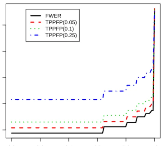
van der Laan et al. [2004], and subsequently Dudoit et al. [2004] and Dudoit and van der Laan [2004], proposeaugmentation multiple testing procedures
(AMTP), obtained by adding suitably chosen null hypotheses to the set of null hypotheses already rejected by an initial gFWER-controlling MTP. Specifically, givenanyinitial procedure controlling the generalized family-wise error rate, augmentation procedures are derived for controlling Type I error rates defined as tail probabilities and expected values for arbitrary functionsg(Vn, Rn) of the numbers of Type I errors and rejected hypotheses
(e.g., proportiong(Vn, Rn) =Vn/Rn of false positives among the rejected
hypotheses). Adjusted p-values for the AMTP are shown to be simply shifted versions of the adjustedp-values of the original MTP. The impor-tant practical implication of these results is that any FWER-controlling MTP and its corresponding adjustedp-values immediately provide multi-ple testing procedures controlling a broad class of Type I error rates and their adjustedp-values. One can therefore build on the large pool of avail-able FWER-controlling procedures, such as the single-step and step-down maxT and minP procedures discussed in Sections 0.2.4 and 0.2.5, above.
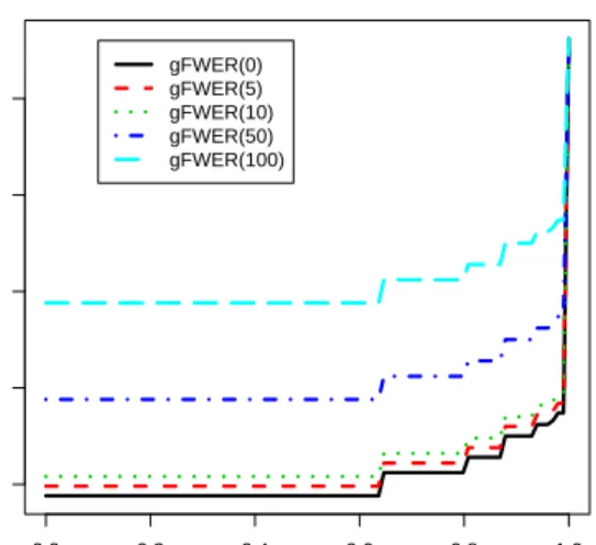
Augmentation procedures for controlling tail probabilities of the num-ber (gFWER) and proportion (TPPFP) of false positives, based on an initial FWER-controlling procedure, are treated in detail in van der Laan et al. [2004] and Dudoit et al. [2004], and are summarized below. The gFWER and TPPFP correspond to the special casesg(Vn, Rn) =Vn and
g(Vn, Rn) =Vn/Rn, respectively.
Denote the adjusted p-values for the initial FWER-controlling procedure Rn(α) by Pe0n(m). Order the M null hypotheses according to these p
-values, from smallest to largest, that is, define indices On(m), so that
e
P0n(On(1)) ≤ . . . ≤ Pe0n(On(M)). Then, for a nominal level α test, the
initial FWER-controlling procedure rejects the following null hypotheses Rn(α)≡ {m:Pe0n(m)≤α}. (19)
Procedure 6 gFWER-controlling augmentation multiple testing procedure
For control of gF W ER(k) at level α, given an initial FWER-controlling procedure Rn(α), reject the Rn(α) = |Rn(α)| null hypotheses specified by
this MTP, as well as the nextAn(α)most significant hypotheses,
The adjustedp-valuesPe0+n(On(m))for the new gFWER-controlling AMTP
are simplyk–shifted versions of the adjusted p-values of the initial FWER-controlling MTP, with the first k adjusted p-values set to zero. That is,
e P0+n(On(m)) = ( 0, if m≤k e P0n(On(m−k)), if m > k . (21)
The AMTP thus guarantees at leastk rejected hypotheses.
Procedure 7 TPPFP-controlling augmentation multiple testing procedure
For control of T P P F P(q) at level α, given an initial FWER-controlling procedure Rn(α), reject the Rn(α) = |Rn(α)| null hypotheses specified by
this MTP, as well as the nextAn(α)most significant hypotheses,
An(α) = max m∈ {0, . . . , M−Rn(α)}: m m+Rn(α) ≤q (22) = min qRn(α) 1−q , M −Rn(α) ,
where the floor bxc denotes the greatest integer less than or equal to x, i.e., bxc ≤ x < bxc+ 1. That is, keep rejecting null hypotheses until the ratio of additional rejections to the total number of rejections reaches the allowed proportion q of false positives. The adjustedp-valuesPe
+
0n(On(m))
for the new TPPFP-controlling AMTP are simply mq–shifted versions of the adjustedp-values of the initial FWER-controlling MTP. That is,
e
P0+n(On(m)) =Pe0n(On(d(1−q)me)), m= 1, . . . , M, (23)
where theceilingdxedenotes the least integer greater than or equal to x.
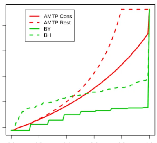
FDR-controlling procedures
Given any TPPFP-controlling procedure, van der Laan et al. [2004] derive two simple (conservative) FDR-controlling procedures. The more general and conservative procedure controls the FDR at nominal levelα, by
control-lingT P P F P(α/2) at level α/2. The less conservative procedure controls
the FDR at nominal levelα, by controllingT P P F P(1−√1−α) at level 1−√1−α. The reader is referred to the original article for details and proofs of FDR control (Section 2.4, Theorem 3). In what follows, we refer to these two MTPs asconservative andrestricted, respectively.
xviii
0.3
Software implementation: R
multtest
package
0.3.1
Overview
The MTPs proposed in Sections 0.2.4 – 0.2.6 are implemented in the lat-est version of the Bioconductor R package multtest (Version 1.6.0). New features include: an expanded class of tests, such as tests for regression pa-rameters in linear models and in Cox proportional hazards models; control of a wider selection of Type I error rates (e.g., gFWER, TPPFP, FDR); bootstrap estimation of the test statistics null distribution; augmentation multiple testing procedures; confidence regions for the parameter vector of interest. Because of their general applicability and novelty, we focus in this section on MTPs that utilize a bootstrap estimated test statistics null distribution and that are available through the package’s main user-level function, MTP. Note that for many testing problems, MTPs based on a permutation (rather than bootstrap) estimated null distribution are also applicable. In particular, FWER-controlling permutation-based step-down maxT and minP MTPs are implemented in the functions mt.maxT and
mt.minP, respectively, and can also be applied directly through a call to
theMTPfunction.
We stress that all the bootstrap-based MTPs implemented in multtest
can be performed using the main user-level function MTP. Note that the
multtest package also provides several simple, marginal FWER-controlling MTPs, such as the Bonferroni, Holm [1979], Hochberg [1988], and ˇSid´ak ˇ
Sid´ak [1967] procedures, and FDR-controlling MTPs, such as the Benjamini & Hochberg [Benjamini and Hochberg, 1995] and Benjamini & Yekutieli [Benjamini and Yekutieli, 2001] step-up procedures. These procedures are available through themt.rawp2adjpfunction, which takes a vector of un-adjustedp-values as input and returns the corresponding adjustedp-values. For greater detail onmulttest functions, the reader is referred to the pack-age documentation, in the form of help files, e.g.,?MTP, and vignettes, e.g.,
openVignette("multtest").
As detailed in Section 0.2.1, above, one needs to specify the following main ingredients when applying a MTP: thedata,X1, . . . , Xn; suitably
de-finedtest statistics,Tn, for each of the null hypotheses under consideration
(e.g., one-samplet-statistics, robust rank-basedF-statistics,t-statistics for regression coefficients in Cox proportional hazards model); a choice ofType I error rate, θ(FVn,Rn), providing an appropriate measure of false
posi-tives for the particular testing problem (e.g., T P P F P(0.10)); a proper
joint null distribution,Q0(or estimate thereof,Q0n), for the test statistics
(e.g., bootstrap null distribution as in the bootstrap procedure of section 1); given the previously defined components, amultiple testing procedure, Rn = R(Tn, Q0n, α), for controlling the error rate θ(FVn,Rn) at a target
Accordingly, themulttest package has adopted a modular and extensible approach to the implementation of MTPs, with the following four main types of functions.
Functions for computing the test statistics, Tn. These are internal
func-tions (e.g.,meanX,coxY), i.e., functions that are generally not called directly by the user. As shown in Section 0.3.2, below, the type of test statistic is specified by thetestargument of the main user-level func-tion MTP. Advanced users, interested in extending the class of tests available in multtest, can simply add their own test statistic func-tions to the existing library of such internal funcfunc-tions (see Section 0.3.4, below, for a brief discussion of the function closure approach for specifying test statistics).
Functions for obtaining the test statistics null distribution, Q0, or an
estimate thereof, Q0n. The main function currently available is the
internal function boot.resample, implementing the non-parametric version of the bootstrap procedure of section 1.
Functions for implementing the multiple testing procedure,Rn=R(Tn, Q0n, α).
The main user-level function is the wrapper functionMTP, which re-turns rejection regions, confidence regions, and adjustedp-values, for MTPs controlling a variety of Type I error rates. In particular, it implements the single-step and step-down maxT and minP proce-dures for FWER control (Sections 0.2.4 and 0.2.5). The functions
fwer2gfwer, fwer2tppfp, and fwer2fdr implement, respectively,
gFWER-, TPPFP-, and FDR-controlling augmentation multiple testing procedures, based on adjusted p-values from any FWER-controlling procedure, and can be called via the typeone argument toMTP(Section 0.2.6).
Functions for numerical and graphical summaries of a MTP.As described in Section 0.3.3, below, a number of summary methods are available to operate on objects of classMTP, output from the mainMTPfunction.
0.3.2
Resampling-based multiple testing procedures:
MTP
function
The main user-level function for resampling-based multiple testing isMTP.
> args(MTP)
function (X, W = NULL, Y = NULL, Z = NULL, Z.incl = NULL, Z.test = NULL, na.rm = TRUE, test = "t.twosamp.unequalvar", robust = FALSE,
standardize = TRUE, alternative = "two.sided", psi0 = 0, typeone = "fwer", k = 0, q = 0.1, fdr.method = "conservative", alpha = 0.05, nulldist = "boot", B = 1000, method = "ss.maxT",
xx
seed = NULL) NULL
INPUT.
Data.The data,X, consist of aJ–dimensional random vector, observed on each ofnsampling units (patients, cell lines, mice, etc.). These data can be stored in aJ×nmatrix,data.frame, orexprs slot of an object of classexprSet. In some settings, aJ–vector of weights may be associ-ated with each observation, and stored in aJ×nweightmatrix,W(or ann–vectorW, if the weights are the same for each of theJ variables). One may also observe a possibly censored continuous or polychoto-mous outcome,Y, for each sampling unit, as obtained, for example, from thephenoDataslot of an object of classexprSet. In some studies, Ladditional covariates may be measured on each sampling unit and stored inZ, ann×L matrix or data.frame. When the tests concern parameters in regression models with covariates from Z (e.g.,
val-ues lm.XvsZ, lm.YvsXZ, and coxph.YvsXZ, for the argument test,
described below), the argumentsZ.inclandZ.testspecify, respec-tively, which covariates (i.e., which columns of Z, including Z.test) should be included in the model and which regression parameter is to be tested (only whentest="lm.XvsZ"). The covariates can be spec-ified either by a numeric column index or character string. If X is an instance of the class exprSet, Y can be a column index or char-acter string referring to the variable in the data.frame pData(X) to use as outcome. Likewise,Z.inclandZ.testcan be column indices or character strings referring to the variables in pData(X)to use as covariates. The argument na.rm controls the treatment of missing values (NA). It isTRUEby default, so that an observation with a miss-ing value in any of the data objects’jth component (j= 1, . . . , J) is excluded from the computation of any test statistic based on thisjth variable.
Test statistics. The test statistics should be chosen based on the pa-rameter of interest (e.g., location, scale, or regression papa-rameters) and the hypotheses one wishes to test. In the current implementa-tion of multtest, the following test statistics are available through the argument test, with default value t.twosamp.unequalvar, for two-sample Welcht-statistics.
• t.onesamp: One-samplet-statistics for tests of means.
• t.twosamp.equalvar: Equal variance two-samplet-statistics for
tests of differences in means.
• t.twosamp.unequalvar: Unequal variance two-samplet-statistics
for tests of differences in means (also known as two-sample Welch t-statistics).
• t.pair: Two-sample pairedt-statistics for tests of differences in means.
• f: Multi-sample F-statistics for tests of equality of population means.
• f.block: Multi-sample F-statistics for tests of equality of
population means in a block design.
• lm.XvsZ:t-statistics for tests of regression coefficients for
vari-able Z.test in linear models each with outcome X[j,] (j =
1, . . . , J), and possibly additional covariates Z.incl from the
matrix Z (in the case of no covariates, one recovers the one-samplet-statistic,t.onesamp).
• lm.YvsXZ:t-statistics for tests of regression coefficients in linear
models with outcomeYand eachX[j,](j= 1, . . . , J) as covari-ate of interest, with possibly other covaricovari-atesZ.incl from the
matrix Z.
• coxph.YvsXZ: t-statistics for tests of regression coefficients in
Cox proportional hazards survival models with outcomeY and
eachX[j,] (j= 1, . . . , J) as covariate of interest, with possibly
other covariatesZ.inclfrom thematrix Z.
Robust,rank-basedversions of the above test statistics can be specified by setting the argumentrobusttoTRUE(the default value isFALSE). Consideration should be given to whether standardized or unstan-dardizeddifference statistics are most appropriate (Equation (1); see Pollard and van der Laan [2004] for a comparison). Both options are available through the argumentstandardize, by defaultTRUE. The type of alternative hypotheses is specified via thealternative argu-ment: default value of two.sided, for two-sided test, and values of
less or greater, for one-sided tests. The (common) null value for
the parameters of interest is specified through thepsi0argument, by default zero.
Type I error rate. The MTPfunction controls by default the FWER (ar-gumenttypeone="fwer"). Augmentation procedures (Section 0.2.6), controlling other Type I error rates such as the gFWER, TPPFP, and FDR, can be specified through the argumenttypeone. Related argu-ments includekandq, for the allowed number and proportion of false positives for control ofgF W ER(k) andT P P F P(q), respectively, and
fdr.method, for the type of TPPFP-based FDR-controlling
proce-dure (i.e.,"conservative"or"restricted"methods). The nominal level of the test is determined by the argumentalpha, by default 0.05. Testing can be performed for a range of nominal Type I error rates by specifying a vector of levelsalpha.
Test statistics null distribution.The test statistics null distribution is es-timated by default using the non-parametric version of the bootstrap
xxii
procedure of section 1 (argumentnulldist="boot"). The bootstrap procedure is implemented in the internal function boot.resample, which calls C to compute test statistics for each bootstrap sample. The values of the shift (λ0) and scale (τ0) parameters are
deter-mined by the type of test statistics (e.g., λ0 = 0 and τ0 = 1
fort-statistics). Permutation null distributions are also available via
nulldist="perm". The number of resampling steps is specified by
the argumentB, by default 1,000.
Multiple testing procedures. Several methods for controlling the chosen Type I error rate are available inmulttest.
• FWER-controlling procedures. The MTP function implements the single-step and step-down (common-cut-off) maxT and (common-quantile) minP MTPs for FWER control, described in Sections 0.2.4 and 0.2.5, and specified through the argument
method (internal functions ss.maxT, ss.minP, sd.maxT, and
sd.minP). The default MTP is the single-step maxT procedure
(method="ss.maxT"), since it requires the least computation.
• gFWER-, TPPFP-, and FDR-controlling augmentation proce-dures. As discussed in Section 0.2.6, any FWER-controlling MTP can be trivially augmented to control additional Type I error rates, such as the gFWER and TPPFP. Two FDR-controlling procedures can then be derived from the TPPFP-controlling AMTP. AMTPs are implemented in the functions
fwer2gfwer, fwer2tppfp, and fwer2fdr, which take FWER
adjusted p-values as input and return augmentation adjusted p-values for control of the gFWER, TPPFP, and FDR, respec-tively. Note that the aforementioned AMTPs can be applied directly via thetypeoneargument of the main functionMTP.
Output control. Various arguments are available to specify which com-bination of the following quantities should be returned: confidence regions (argumentget.cr); cut-offs for the test statistics (argument
get.cutoff); adjustedp-values (argumentget.adjp); test statistics
null distribution (argument keep.nulldist). Note that parameter estimates and confidence regions only apply to the test of single-parameter null hypotheses (i.e., not theF-tests). In addition, in the current implementation ofMTP, parameter confidence regions and test statistic cut-offs are only provided when typeone="fwer", so that
get.crandget.cutoffshould be set toFALSEwhen using the error
rates gFWER, TPPFP, or FDR.
The S4 class/method object-oriented programming approach was adopted to summarize the results of a MTP (Section 0.3.4). The output of theMTP
function is an instance of theclass MTP, with the followingslots,
> slotNames("MTP")
[1] "statistic" "estimate" "sampsize" "rawp" "adjp" "conf.reg" [7] "cutoff" "reject" "nulldist" "call" "seed"
MTP results.An instance of theMTPclass contains slots for the following MTP results:
• statistic: The numeric M–vector of test statistics, specified
by the values of theMTPargumentstest,robust,standardize, andpsi0. In many testing problems,M =J =nrow(X).
• estimate: For the test of single-parameter null hypotheses
us-ingt-statistics (i.e., not the F-tests), the numeric M–vector of estimated parameters.
• sampsize: The sample size, i.e., n=ncol(X).
• rawp: The numericM–vector of unadjustedp-values.
• adjp: The numeric M–vector of adjusted p-values (computed only if theget.adjpargument isTRUE).
• conf.reg: For the test of single-parameter null hypotheses
us-ing t-statistics (i.e., not the F-tests), the numeric M × 2×
length(alpha) array of lower and upper simultaneous
confi-dence limits for the parameter vector, for each value of the nominal Type I error ratealpha(computed only if theget.cr
argument isTRUE).
• cutoff: The numericM×length(alpha)matrix of cut-offs for
the test statistics, for each value of the nominal Type I error rate
alpha(computed only if theget.cutoffargument isTRUE).
• reject: The M× length(alpha) matrix of rejection
indica-tors (TRUE for a rejected null hypothesis), for each value of the nominal Type I error ratealpha.
Null distribution. Thenulldistslot contains the M×B matrix for the estimated test statistics null distribution. This slot is returned only if
keep.nulldist=TRUE; option not currently available for permutation
null distribution, i.e.,nulldist="perm". By default (i.e., for
nulld-ist="boot"), the entries of nulldistare the null value shifted and
scaled bootstrap test statistics, as defined in the bootstrap procedure of section 1.
Reproducibility.The last two slots of anMTP object provide information on the particular call to theMTPfunction and can be used for repro-ducibility in a repeat call toMTP. The slotcallcontains the call to the functionMTP, andseedis an integer specifying the state of the random number generator used to create the resampled datasets. The seed
ar-xxiv
gument is currently used only for the bootstrap null distribution (i.e., fornulldist="boot").
0.3.3
Numerical and graphical summaries
The following methods were defined to operate on MTP instances and summarize the results of a MTP.
print: Theprintmethod returns a description of an object of classMTP,
including the sample sizen, the numberM of tested hypotheses, the type of test performed (value of argumenttest), the Type I error rate (value of argumenttypeone), the nominal level of the test (value of argumentalpha), the name of the MTP (value of argumentmethod), the call to the functionMTP. In addition, this method produces a table with the class, mode, length, and dimension of each slot of theMTP
instance.
summary: The summary method provides numerical summaries of the
results of a MTP and returns a list with the following three components:
• rejections: A data.frame with the number(s) of rejected
hy-potheses for the nominal Type I error rate(s) specified by the
alpha argument of the functionMTP (NULL values are returned
if all three argumentsget.cr, get.cutoff, and get.adjp are
FALSE).
• index: A numericM–vector of indices for ordering the
hypothe-ses according to first adjp, thenrawp, and finally the absolute value of statistic(not printed in the summary).
• summaries: When applicable (i.e., when the corresponding
quan-tities are returned byMTP), a table with six number summaries of the distributions of the adjusted p-values, unadjusted p-values, test statistics, and parameter estimates.
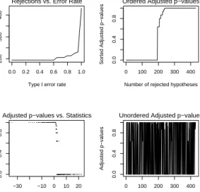
plot: The plot method produces the following graphical summaries of the results of a MTP. The type of display may be specified via the
whichargument.
1. Scatterplot of number of rejected hypotheses vs. nominal Type I error rate.
2. Plot of ordered adjusted p-values; can be viewed as a plot of Type I error rate vs. number of rejected hypotheses.
3. Scatterplot of adjusted p-values vs. test statistics (also known as “volcano plot”).
4. Plot of unordered adjustedp-values.
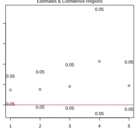
5. Plot of confidence regions for user-specified parameters, by de-fault the 10 parameters corresponding to the smallest adjusted p-values (argumenttop).
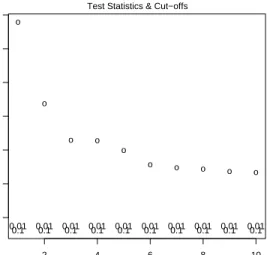
6. Plot of test statistics and corresponding cut-offs (for each value of alpha) for user-specified hypotheses, by default the 10 hypotheses corresponding to the smallest adjusted p-values (argumenttop).
The argument logscale (by default equal to FALSE) allows one to use the negative decimal logarithms of the adjusted p-values in the second, third, and fourth graphical displays. Note that some of these plots are implemented in the older functionmt.plot.
[: Subsetting method, which operates selectively on each slot of anMTP
instance to retain only the data related to the specified hypotheses.
as.list: Converts an object of classMTP to an object of classlist, with
an entry for each slot.
0.3.4
Software design
The following features of the programming approach employed inmulttest
may be of interest to users, especially those interested in extending the functionality of the package.
Function closures.The use offunction closures, as in thegenefilter pack-age, allows uniform data input for all MTPs and facilitates the extension of the package’s functionality by adding, for example, new types of test statistics. Specifically, a function closure is defined for each value of the
MTPargumenttest. The closure consists of a function for computing the test statistic (with only two arguments, a data vectorxand a corresponding weight vectorw, with default value of NULL) and its enclosing environment, with bindings for relevant additional arguments, such as null valuespsi0, outcomesY, and covariatesZ. Existing internal test statistic functions are located in the fileR/statistics.R. Thus, new test statistics can be added to multtest by simply defining a new closure and adding a corresponding value for thetestargument toMTP.
Class/method object-oriented programming.Like many other Bio-conductor packages, multtest has adopted the S4 class/method object-oriented programming approach of Chambers [1998]. In particular, a new class,MTP, and associated methods, were defined to represent and operate on the results of multiple testing procedures.
Calls to C. Because resampling procedures, such as the non-parametric bootstrap implemented in multtest, are computationally intensive, care must be taken to ensure that the resampling steps are not prohibitively slow. The use of function closures for the test statistics, however, prevents writing the entire program in C. In the current implementation, we have
xxvi
chosen to define the closure and compute the observed test statistics in R, and then call C to apply the closure to each bootstrap resampled dataset (using the R random number generator). This approach puts the for loops over bootstrap samples (B) and hypotheses (M) in the compiled code, thus speeding up this computationally expensive part of the program.
0.4
Applications: ALL microarray dataset
0.4.1
ALL data package and initial gene filtering
We illustrate some of the functionality of the multtest package using the Acute Lymphoblastic Leukemia (ALL) microarray dataset of Chiaretti et al. [2004], available in the data package ALL. The main object in this package isALL, an instance of the classexprSet. The genes-by-subjects ma-trix of 12,625 Affymema-trix expression measures (chip series HG-U95Av2) for each of 128 ALL patients is provided in the exprs slot of ALL. The
phenoData slot contains 21 phenotypes (i.e., patient level responses and
covariates) for each patient. Note that the expression measures have been obtained using the three-step robust multichip average (RMA) preprocess-ing method, implemented in the packageaffy. In particular, the expression measures have been subject to a base 2 logarithmic transformation. For greater detail, please consult theALLpackage documentation.
> library("ALL") > library("hgu95av2") > data(ALL)
Our goal is to identify genes whose expression measures are associated with (possibly censored) biological and clinical outcomes such as: tumor cellular subtype (B-cell vs. T-cell), tumor molecular subtype (BCR/ABL, NEG, ALL1/AF4), and time to relapse. Alternative analyses of this dataset are discussed in Chapters??,??,??,??, and??. Before applying the MTPs, we perform initial gene filtering as in Chiaretti et al. [2004] and retain only those genes for which: (i) at least 20% of the subjects have a measured intensity of at least 100 and (ii) the coefficient of variation (i.e., the ratio of the standard deviation to the mean) of the intensities across samples is between 0.7 and 10. These two filtering criteria can be readily applied using functions from thegenefilter package.
> ffun <- filterfun(pOverA(p = 0.2, A = 100), cv(a = 0.7, b = 10)) > filt <- genefilter(2^exprs(ALL), ffun)
> filtALL <- ALL[filt, ]
> filtX <- exprs(filtALL) > pheno <- pData(filtALL)
The new filtered dataset, filtALL, contains expression measures on 431 genes, for 128 patients.
0.4.2
Association of expression measures and tumor cellular
subtype: two-sample
t
-statistics
FWER-controlling step-down minP MTP with two-sample Welch
t-statistics and bootstrap null distribution
Different tissues are involved in ALL tumors of the B-cell and T-cell sub-types. The phenotypic data include a variable,BT, which encodes the tissue type and stage of differentiation. In order to identify genes with higher mean expression measures in B-cell ALL patients compared to T-cell ALL pa-tients, we create an indicator variable,Bcell(1 for B-cell, 0 for T-cell), and compute, for each gene, a two-sample Welch (unequal variance)t-statistic. We choose to control the FWER using the bootstrap-based step-down minP procedure with B = 100 bootstrap iterations, although more bootstrap iterations are recommended in practice.
> table(pData(ALL)$BT)
B B1 B2 B3 B4 T T1 T2 T3 T4
5 19 36 23 12 5 1 15 10 2
> Bcell <- rep(0, length(pData(ALL)$BT))
> Bcell[grep("B", as.character(pData(ALL)$BT))] <- 1
> seed <- 99
> BT.boot <- MTP(X = filtX, Y = Bcell, alternative = "greater", + B = 100, method = "sd.minP", seed = seed)
running bootstrap... iteration = 100
Let us examine the results of the MTP stored in the objectBT.boot.
> summary(BT.boot)
MTP: sd.minP
Type I error rate: fwer
Level Rejections
1 0.05 194
Min. 1st Qu. Median Mean 3rd Qu. Max.
adjp 0.000 0.0000 0.8700 0.5314 1.0000 1.000
rawp 0.000 0.0000 0.0300 0.3559 0.9450 1.000
statistic -34.420 -1.5690 2.0120 2.0590 5.3830 22.330