Statistical Modelling for Exposure
Measurement Error with Application to
Epidemiological Data
Thesis Committee
Promotors
Prof. dr. Hendriek C. Boshuizen
Professor in Biostatistic Modelling in Nutrition Research Division of Human Nutrition, Wageningen University Prof. dr. Fred A. van Eeuwijk
Professor of Applied Statistics Biometris, Wageningen University
Co-promotor
Dr. Hilko van der Voet DLO Researcher, Biometris
Wageningen University and Research Centre
Other members
Prof. dr. ir. E.J.M. Feskens, Wageningen University Dr. S. Le Cessie, Leiden University
Prof. dr. J. Wallinga, Leiden University
Dr. R.H. Keogh, London School of Hygiene and Tropical Medicine
This research was conducted under the auspices of the Graduate School VLAG (Advanced studies in Food Technology, Agrobiotechnology, Nutrition and Health Sciences).
Measurement Error with Application to
Epidemiological Data
George O. Agogo
Thesis
submitted in fulfilment of the requirements for the degree of doctor at Wageningen University
by the authority of the Rector Magnificus Prof. Dr A.P.J. Mol,
in the presence of the
Thesis Committee appointed by the Academic Board to be defended in public
on Thursday 14 January 2016 at 11:00 a.m. in the Aula.
George O. Agogo
Statistical Modelling for Exposure Measurement Error with Application to Epidemiological Data, 160 pages.
PhD thesis, Wageningen University, Wageningen, NL (2016) With references, with summaries in English
i
Abstract
Background Measurement error in exposure variables is an important issue in
epidemiological studies that relate exposures to health outcomes. Such studies, however, usually pay limited attention to the quantitative effects of exposure measurement error on estimated exposure-outcome associations. Therefore, the estimators for exposure-outcome associations are prone to bias. Existing methods to adjust for the bias in the associations require a validation study with multiple replicates of a reference measurement. Validation studies with multiple replicates are quite costly and therefore, in some cases only a single–replicate validation study is conducted besides the main study. For a study that does not include an internal validation study, the challenge in dealing with exposure measurement error is even bigger. The challenge is how to use external data from other similar validation studies to adjust for the bias in the exposure-outcome association. In accelerometry research, various accelerometer models have currently been developed. However, some of these new accelerometer models have not been properly validated in field situations. Despite the widely recognized measurement error in the accelerometer, some accelerometers have been used to validate other instruments, such as physical activity questionnaires, in measuring physical activity. Consequently, if an instrument is validated against the accelerometer, and the accelerometer itself has considerable measurement error, the observed validity in the instrument being validated will misrepresent the true validity.
Methodology In this thesis, we adapted regression calibration to adjust for exposure
measurement error for a single-replicate validation study with zero-inflated reference measurements and assessed the adequacy of the adapted method in a simulation study. For the case where there is no internal validation study, we showed how to combine external data on validity for self-report instruments with the observed questionnaire data to adjust for the bias in the associations caused by measurement error in correlated exposures. In the last part, we applied a measurement error model to assess the
ii
Results The performance of the proposed two-part model was sensitive to the form of
continuous independent variables and was minimally influenced by the correlation between the probability of a non-zero response and the actual non-zero response values. Reducing the number of covariates in the model seemed beneficial, but was not critical in large-sample studies. We showed that if the confounder is strongly linked with the outcome, measurement error in the confounder can be more influential than measurement error in the exposure in causing the bias in the exposure-outcome association, and that the bias can be in any direction. We further showed that when accelerometers are used to monitor the level of physical activity in free-living individuals, the mean level of physical activity would be underestimated, the associations between physical activity and health outcomes would be biased, and there would be loss of statistical power to detect associations.
Conclusion The following remarks were made from the work in this thesis. First, when
only a single-replicate validation study with zero-inflated reference measurements is available, a correctly specified regression calibration can be used to adjust for the bias in the exposure-outcome associations. The performance of the proposed calibration model is influenced more by the assumption made on the form of the continuous covariates than the form of the response distribution. Second, in the absence of an internal validation study, carefully extracted validation data that is transportable to the main study can be used to adjust for the bias in the associations. The proposed method is also useful in conducting sensitivity analyses on the effect of measurement errors. Lastly, when “reference” instruments are themselves marred by substantial bias, the effect of measurement error in an instrument being validated can be seriously underestimated.
iii Table of Contents
1 Introduction 1
2 Use of two-part regression calibration model to correct for measurement error in episodically consumed foods in a single-replicate study design: EPIC Case Study 17 3 Evaluation of a two-part regression calibration to adjust for dietary exposure measurement error in the Cox proportional hazards model: a simulation study 43 4 A multivariate method to correct for Measurement Error in Exposure variables
using External validation Data 69
5 Quantification of Measurement Errors in Accelerometer Physical Activity Data 93
6 General discussion 113
Glossary 134
References 137
Summary 147
Acknowledgements 151
About the Author 155
1
1
Introduction
1.1
Measurement error in exposure variables
Measurement error in exposure variables is a known problem in many research areas. By definition, measurement error refers to the discrepancy between the true value and measured value of a variable (Thomas, Stram and Dwyer, 1993). In epidemiological research, measurement error can be due to recall bias when studies are conducted retrospectively requiring an individual to recall and report past events, or due to biological variations and instrument errors in laboratory experiments. Measurement error in exposures has been a long-term concern in relating exposures to health outcomes in epidemiological studies (Rothman, Greenland and Lash, 2008). In nutritional epidemiology, measurement error in dietary exposures has been a major impediment in relating long-term dietary intake to the occurrence of a disease (Ferrari et al., 2008). For example, the interest might be in the association between long-term intake of fruit and vegetable (hereafter, FV) and overall risk of cancer, as is the case in Boffetta et al. (2010). In such studies, dietary intake is usually assessed with a report instrument, which is prone to measurement error. Measurement error in the self-report instrument can be due to memory failure to recall past intakes over a long period of time (Agudo, 2004; Rosner and Gore, 2001). Therefore, it is impossible to measure long-term intake exactly.
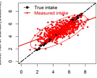
Using a dietary example, measurement error in dietary exposures can have two important effects in the parameter estimate that relates dietary intake to occurrence of a disease (Carroll et al., 2006). First, measurement error in dietary exposure can bias the parameter estimate that quantifies the association between dietary intake and occurrence of a disease (hereafter, diet-disease association). Second, there can be loss of statistical power to detect existing diet-disease associations. To illustrate these two important effects of measurement error, we use simulated data on the association between FV intake and reduction in the risk of cancer as an example (Figure 1.1).
2
Random measurement error in FV intake leads to scatterplots (diamond dots) that are either higher or lower than true values (round dots). As a result, the regression slope that quantifies the association between FV intake and lower risk of cancer becomes more flattened (solid line) than the true slope (dashed line). This flattening effect quantifies the attenuation due to measurement error in the exposure. Attenuation refers to the bias of the association toward the null (Kipnis et al., 2003). Additionally, the variability around the regression line is much greater when the measured intake is used (diamond dots) than the variability around the regression line when the true intake is used (round dots), demonstrating loss of statistical power. The implication of the loss of power is that larger sample sizes are required to detect associations.
Figure 1.1: Simulated data showing the two important effects of measurement error on the association between reduction of risk of cancer (outcome) and FV intake (exposure): bias in the exposure-outcome association (attenuation) and loss of statistical power to detect associations. True intake (exposure) is shown by round dots and measured intake by diamond dots.
The focus of this thesis is on methods to adjust for the bias in the exposure-outcome associations, when exposure variables are measured with errors. When multiple
3
exposures are measured with correlated errors, the exposure-outcome association can be biased in any direction (Day et al., 2004; Michels et al., 2004; Rosner et al., 2008). The exposure measurement error problem has prompted much methodological research, initially, on understanding the effects of measurement error on exposure-outcome associations and, more recently, on developing statistical methods to correct for exposure measurement error (Buonaccorsi, 2010; Carroll et al., 2006).
1.2
Measurement error in dietary exposure assessment
The commonly used self-report instruments for measuring dietary intakes include food dietary questionnaires (DQs), 24-hour dietary recalls (24HRs) and dietary records (Agudo, 2004; Black, Welch and Bingham, 2000). In measuring dietary intake with a DQ, a wide range of food items are listed and individuals are asked to report their average frequency of consumption and average amount consumed over a long period of time, typically between several months to a year. A major drawback associated with the use of the DQ is memory failure to recall past intake. In the 24HR, however, subjects are asked to report their intake within 24 hours prior to the assessment time. Similar to the DQ, 24HR is also prone to recall bias, but to a lesser extent. Additionally, a single 24HR is unreliable in measuring long-term intake, unless administered multiple times per individual (Agudo, 2004). Unlike DQ and 24HR, in dietary records, an individual keeps a record of actual intake of foods consumed at the time of consumption for a specified period (Willet, 1998). Measuring food intake with the dietary record can lead to individuals changing their food intake patterns, when they realize that their intake is being monitored. This could lead to misreporting of true intake in the dietary record (Johnson, 2002). Further details on dietary assessment methods can be found in Al-Delaimy et al. (2005), Bingham et al. (1997), Bingham et al. (1994) and Block (1982, 1989).
1.3
Common measurement error terminologies, types and
structures
Measurement error can either be systematic or random. Systematic error arises when an individual consistently overestimates or underestimates his true level of exposure
4
(Agudo, 2004). Random error, however, arises when an individual sometimes overestimates and sometimes underestimates true level of exposure.
Exposure measurement error can either be nondifferential or differential. Nondifferential error occurs when the measured exposure contains no extra information about the health outcome other than what is contained in true exposure; error is said to be differential otherwise (Carroll et al., 2006, p. 36). In the FV intake-cancer example, if measurement error is nondifferential, measured FV intake in a single day should not contribute extra information about the risk of cancer other than what is contained in true long-term FV intake. On the other hand, if measurement error in reported FV intake depends upon whether an individual has cancer or not, especially due to recall bias when such a study is conducted retrospectively, then the measurement error will be differential (Thomas et al., 1993).
To define different types of measurement error using the FV intake example, we denote self-report intake by 𝑄𝑄, unknown long-term true intake by 𝑇𝑇 and measurement error in self-reported intake by 𝜀𝜀𝑄𝑄.
Measurement error structure can either be of classical or Berkson type. Classical error occurs when true intake is measured with error, such that the variability in the measured intake is greater than the variability in true intake. An example of classical measurement error structure is given by
𝑄𝑄=𝑇𝑇+𝜀𝜀𝑄𝑄. (1.1)
Berkson error, on the other hand, occurs when true intake is the sum of measured intake and measurement error, such that the variability in true intake is greater than the variability in the measured intake (Berkson, 1950). An example of Berkson error structure is given by
𝑇𝑇=𝑄𝑄+𝜀𝜀𝑄𝑄. (1.2)
An example where Berkson error occurs is when individuals are classified into groups and all group members are assigned the same exposure value, say, the mean of true intake within that group; however, true intake for individuals within the same group
5
would differ from the assigned intake values (Thomas et al., 1993). Exposures can also be measured with a mixture of Berkson and classical error as shown in Carroll et al. (2006, p. 51).
The structure of measurement error can either be additive (as in expression (1.1)) or multiplicative. Multiplicative error arises when the magnitude of error increases with the quantity of true intake, such that larger true intake values are measured with larger error (Guolo and Brazzale, 2008). Multiplicative error is usually common with dietary intakes (Carroll et al., 2006). An example of a multiplicative measurement error structure can be given as
𝑄𝑄=𝑇𝑇𝜀𝜀𝑄𝑄. (1.3)
Exposure measurements can either be unbiased (e.g., as shown in expression (1.1)) or biased. Intake measurements are biased if the average value does not equal the true mean value, meaning that there is systematic error in Q.
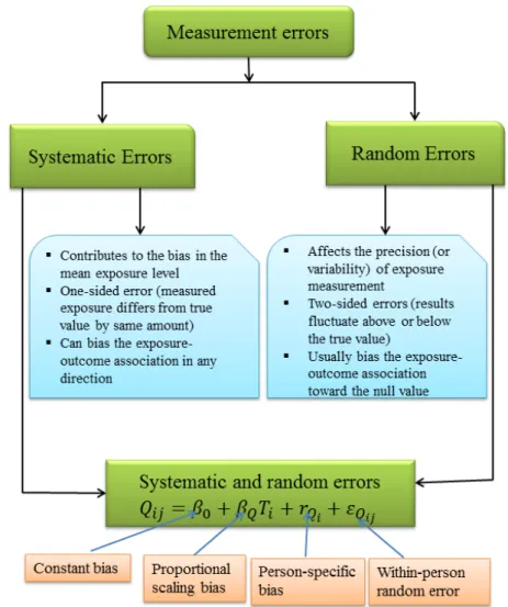
With multiple replicate self-report measurements (denoted by jfor replicate and ifor an individual), an example of additive measurement error structure with both systematic and random error components can be given by
𝑄𝑄𝑖𝑖𝑖𝑖 =𝛽𝛽0+𝛽𝛽𝑄𝑄𝑇𝑇𝑖𝑖+𝑟𝑟𝑄𝑄𝑖𝑖+𝜀𝜀𝑄𝑄𝑖𝑖𝑖𝑖, (1.4)
where 𝛽𝛽0 quantifies overall constant bias and 𝛽𝛽𝑄𝑄 quantifies overall bias that is related to the level of intake (Kipnis et al., 2001); 𝑟𝑟𝑄𝑄𝑖𝑖 is referred to as person-specific bias and describes the fact that two individuals who consume the same amount of food will systematically report their intakes differently (Carroll et al., 2006). For further details on measurement error structures, see Buonaccorsi (2010), Carroll et al. (2006) and Fuller (2006).
In Figure 1.2, systematic and random measurement errors are juxtaposed; also shown are the components of an additive measurement error structure that is shown in expression (1.4).
6
Figure 1.2 Schematic representation of common measurement error structures: systematic, random and both errors.
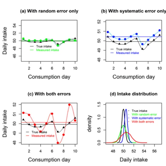
In Figure 1.3, the additive measurement error structures are presented graphically using an example of simulated intake data for an individual. In each graph, the solid horizontal lines represent an individual’s usual intake, defined as the average intake for the ten consumption days. When daily intake is measured with random error only, usual intake is measured accurately, i.e., with no bias as shown in Figure 1.3(a), but imprecisely leading to an inflated variance as shown by wider width of the green solid
7
density curve in Figure 1.3(d). Figure 1.3(b) shows a situation where intake is measured with systematic error (here, constant bias only), and in this case intake is consistently overestimated with a distribution that is shifted to the right of the true distribution, but with the same variance as for the true intake (Figure 1.3(d), blue solid curve). In other cases, however, systematic error can lead to consistent underestimation of intake. Further, when intake is measured with both systematic and random errors, daily intake might be sometimes overestimated and sometimes underestimated, leading to an upward bias in the usual intake as shown in Figure 1.3(c) and an inflated variance as shown in Figure 1.3(d), red solid curve. In other cases, however, where intake is measured with both systematic and random errors, usual intake can be underestimated or overestimated. The wavy lines represent within-individual variation in daily intakes (Figure 1.3(a), (b) and (c)).
8
Figure 1.3: A graphical representation of three common types of additive measurement error structures using simulated data when daily intake is measured with random error only, systematic error only and both systematic and random error. The horizontal lines represent usual intake; the black dots represent true intake values per consumption day; the dots in other colours represent measured intake values. Figure 1.3(d) compares an individual’s daily intake distributions for true intake and measured intakes.
1.4
Common methods to correct for measurement error in
continuous exposures
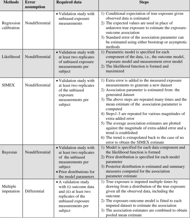
Five common bias-adjustment methods are described in this section. They are summarized in Table 1.1.
9
1.4.1 Regression calibration
Regression calibration is the most commonly used method to adjust for the bias in the exposure-outcome associations caused by measurement errors in the exposure variables (Freedman et al., 2008; Guolo and Brazzale, 2008; Messer and Natarajan, 2008; Rosner, Spiegelman and Willett, 1990; Rosner, Willett and Spiegelman, 1989). This method is widely used because of its simplicity. The general idea of regression calibration is to estimate the conditional expectation of true exposure given the exposure measured with error and other covariates assumed to be measured without error. The estimated expected values are used in place of the unknown true exposure to estimate the association between the exposure and an outcome. Application of regression calibration requires additional information on the unobserved true exposure. This information is usually obtained from a validation study with unbiased measurements for true exposure (Kipnis et al., 1999; Kipnis et al., 2003). A validation study is often smaller than the main study and can be a random sample of subjects in the main study. To apply regression calibration, measurement error in the exposure is assumed to be nondifferential (Keogh and White, 2014). The method usually leads to consistent estimators of the association parameter (Guolo and Brazzale, 2008).
1.4.2 Likelihood method
The use of the likelihood method to correct for exposure measurement error requires specification of a parametric model for every component of the data, namely, the relation between the outcome of interest and the true exposure (hereafter, disease model), the relation between true exposure and covariates such as age and BMI (hereafter, exposure model) and the relation between measured exposure and the true exposure (hereafter, measurement error model). Subsequently, the likelihood function is obtained by integrating the product of the three densities over the latent true exposure variable (Guolo and Brazzale, 2008). The likelihood function is maximized to estimate the model parameters using either numerical methods or analytical approximations (Guolo and Brazzale, 2008). The method requires a validation study with multiple replicates of the unbiased measurements in order to specify the distribution of the true exposure. The likelihood method assumes nondifferential error
10
(Thoresen and Laake, 2000). If correctly specified, the likelihood method can be more efficient than simpler measurement error correction methods such as regression calibration. This method, however, is rarely used in practice due to its computational burden and difficulty to specify parametric assumptions correctly. Moreover, it is often difficult to understand robustness of the likelihood method to model assumptions (Carroll et al., 2006).
1.4.3 Simulation Extrapolation (SIMEX)
SIMEX is a simulation-based method, sharing the simplicity and generality of regression calibration, but can be computationally prohibitive (Carroll et al., 2006). The method was proposed by Cook and Stefanski (1994) and has been developed further (Carroll et al., 1996; Lin and Carroll, 1999; Stefanski and Cook, 1995). The SIMEX method requires knowledge of the measurement error variance. Thus, a validation study with at least two replicates of the unbiased measurements is required. The following steps are followed to adjust for the bias in the association using the SIMEX method (Carroll et al., 2006). First, extra measurement error is added to the exposure measurements, creating a dataset with larger measurement error variance; this data generation step is repeated a large number of times. Second, the disease model is fitted and the association parameter estimated from each of the generated datasets in step one, then the average of the association parameter estimate is computed. Third, the above steps are repeated by adding various magnitudes of extra measurement error. Fourth, the average parameter estimates are plotted against the magnitude of added measurement error variance and then an extrapolant function is fitted. Lastly, the extrapolation is done to the ideal case of no measurement error to obtain the bias-corrected estimate. The method assumes nondifferential error and is well suited for exposures measured with additive or multiplicative error (Guolo and Brazzale, 2008).
1.4.4 Bayesian methods
Bayesian methods have been used to adjust for measurement error in the covariates (Dellaportas and Stephens, 1995; Huang, Chen and Dagne, 2011). To adjust for the exposure measurement error with the Bayesian method, the following steps are followed (Carroll et al., 2006, p. 206-207). Similar to the likelihood method, a
11
parametric model is specified for each component of the data and a likelihood function is formed. In the Bayesian framework, the parameters are assumed as random, unlike in the likelihood method where the parameters are assumed as fixed. Prior distributions are specified for the parameters in the model. Lastly, the posterior summary measures for the association parameter estimates are computed. The computation can be done with either a flexible sampling-based Markov chain Monte Carlo (MCMC) (Gelman and Hill, 2007) or a more computationally efficient non-sampling based integrated nested Laplace approximation (INLA) (Muff, 2015; Rue, Martino and Chopin, 2009). Despite the flexibility of Bayesian MCMC, it can be computationally intensive. Similar to the likelihood method, application of Bayesian method requires a validation study with multiple replicates of the unbiased measurements in order to specify the distribution of the true exposure. The method is suitable for nondifferential errors.
1.4.5 Multiple Imputation
Multiple imputation is a standard technique for handling data that are missing at random (Rubin, 1987). This method was proposed to adjust for measurement error in continuous exposures (Cole, Chu and Greenland, 2006; Freedman et al., 2008). To apply the multiple imputation method, the true exposure is assumed as missing data and is imputed multiple times by drawing from a distribution of the true exposure given all the observed data, including the outcome (Keogh and White, 2014). The multiple imputation method can accommodate differential error, because true exposure is imputed dependent on the outcome. The conditional distribution of the true exposure given the outcome and other observed data is often unknown. To estimate this conditional distribution, a validation study is required with data on (a) the study outcome and (b) multiple replicates of the unbiased measurements per individual. Using the estimated conditional distribution, the true exposure is imputed multiple times per individual to account for the uncertainty in the imputed exposure values. To each imputed dataset, the exposure-outcome model is fitted and the resulting association estimates are combined to obtain a pooled mean estimate (Rubin, 1987). The pooled mean estimate yields the bias-corrected estimator for the true exposure-outcome association (Messer and Natarajan, 2008).
12
Table 1.1: Summary details for common measurement error adjustment methods
Methods Error
assumption
Required data Steps
Regression calibration
Nondifferential
•Validation study with unbiased exposure measurements
1)Conditional expectation of true exposure given observed data is estimated
2)The expected values are used in place of unknown true exposure to estimate the exposure-outcome association
3)Standard error of the association parameter can be estimated using either bootstrap or asymptotic methods
Likelihood Nondifferential
•Validation study with at least two replicates of unbiased exposure measurements per subject
1)Parametric model is specified for each
component of the data, i.e., the outcome model, exposure model and measurement error model 2)The likelihood function is formed and
maximized
SIMEX Nondifferential
•Validation study with at least two replicates of the unbiased exposure
measurements per subject
1)Extra error is added to the measured exposure measurements to generate a new dataset 2)Association parameter is estimated from the
generated dataset
3)The above steps are repeated many times and the mean estimate of the association parameter is computed
4)Steps1-3 are repeated for various magnitudes of extra-added error
5)The average association estimates are plotted against the magnitude of extra-added error and a trend is established
6)The trend is extrapolated back to the case of no error to obtain the SIMEX estimate
Bayesian Nondifferential
•Validation study with at least two replicates of the unbiased measurements per subject
•Prior distributions for the model parameters
1)Model is specified for each data component and the likelihood function is formed
2)Prior distribution is specified for each model parameter
3)Posterior distribution is estimated and summary measures computed for the association
parameter estimate Multiple
imputation Differential
•A validation study with (i) outcome data and (ii) at least two replicates of the unbiased exposure measurements per subject
1)True exposure is imputed multiple times by drawing from a distribution of the true exposure given all the observed data, including the outcome
2)The exposure-outcome model is fitted to each imputed dataset to estimate the association 3)The association estimates are combined to obtain
13
1.5
Current challenges
Most validation studies in nutritional research stop at describing the correlation of measured intake with true intake. Studies that look at the quantitative effects of measurement error in dietary intakes on estimated associations between intake and health outcomes are rare. Additionally, the effects of dietary intakes on health outcomes are usually weak and are marred by inconsistencies. These inconsistencies are partly due to measurement error in intake, because many nutritional studies are based on questionnaires or interviews that contain a large amount of measurement error.
Conducting a multiple-replicate validation study, besides the main study, however, is limited because it is costly. As a result, some epidemiological studies either conduct a single–replicate validation study or do not conduct a validation study at all. Among the commonly used measurement error correction methods (see Table 1.1) only regression calibration can be used for single-replicate calibration studies. However, regression calibration has not been applied and evaluated for a single-replicate validation study with zero-inflated measurements for the calibration response.
For a study that does not include an internal validation study, the challenge in dealing with exposure measurement error is even bigger. The challenge is how to use external validation data from other similar studies to adjust for the bias in the exposure-outcome association. When exposures are measured with correlated errors, it can be very difficult to predict the direction and strength of the association (Marshall, Hastrup and Ross, 1999). The difficulty is due to contamination effect of the confounder measurement error (Freedman et al., 2011). Even though the problem due to contamination effect has been widely acknowledged in the literature, there is a lack of practical methods to quantify this effect in a specific epidemiologic study, both in terms of the approximate magnitude of the effect, and its direction. Measurement error problem is also common in physical activity research, where instruments, such as physical activity questionnaires, physical activity recalls and accelerometers, are used to monitor an individual’s long-term level of physical activity (Ferrari, Friedenreich
14
and Matthews, 2007; Hills, Mokhtar and Byrne, 2014; Lim et al., 2015; Nusser et al., 2012; Tooze et al., 2013). Regarding the accelerometry research, various accelerometer models have currently been developed. However, some of these new accelerometer models have not been properly validated in field situations. Despite the widely recognized measurement error in the accelerometer, some accelerometers have been used to validate other instruments, such as physical activity questionnaires, in measuring physical activity (Lim et al., 2015). Therefore, if an instrument is validated against the accelerometer, and the accelerometer itself has considerable measurement error, the observed validity in the instrument being validated will misrepresent the true validity.
These challenges constitute the motivation for the work in this thesis. The work in this thesis will address the following research questions emanating from the above-mentioned challenges:
(i) When only a single-replicate validation study with zero-inflated measurements is available, can the current methods be adapted to adjust for exposure measurement error?
(ii) When there is no internal validation study, can a practical method be proposed that uses external validation data to adjust for the bias in the exposure-outcome associations?
(iii) How large is the error in physical activity as measured by an accelerometer in free-living individuals and what is the impact of this error when accelerometer is used to validate other instruments?
1.6
Objectives of the study
The research in this thesis aims to address the aforementioned research questions. The key objectives of this thesis are highlighted below:
1) To propose a two-part regression calibration to adjust for measurement error in dietary intakes not consumed daily, when only a single-replicate validation study is
15
available. The task is to start with a simple linear calibration model and then improve it gradually. The improvement is done by modelling the excess zeros explicitly, handling heteroscedasticity in the response, exploring the optimal variable selection criteria, and identifying the optimal parametric forms of the continuous covariates in the calibration model,
2) To assess the performance of the proposed two-part regression calibration model in a simulation study with respect to: the percentage of excess zeroes in the response variable, the magnitude of correlation between probability of a non-zero response and the actual non-zero value, percentage of zeroes in the response and the magnitude of measurement error in the exposure,
3) To develop a multivariate method to adjust for the bias in the exposure-outcome association in the presence of mismeasured confounders when there is no internal validation study. The method combines external data on the validity of self-report instruments with the observed data to adjust for the bias in the exposure-outcome association, while simultaneously adjusting for confounding and measurement error in the confounders,
4) To validate a triaxial accelerometer in a recently concluded study by applying a measurement error model and quantifying the effects of measurement error in physical activity as measured by the accelerometer.
1.7
Thesis outline
This thesis is organized into chapters. The contents of the remaining chapters are summarized below.
In chapter 2, a two-part regression calibration model, initially developed for a
multiple-replicate validation study design, is adapted to a case of a single-replicate validation study. The chapter further describes how to: handle the excess zeroes in the response, using two-part modelling approach; explore optimal parametric forms of the continuous covariates, using generalized additive modelling and empirical logit approaches, and how to select covariates into the calibration model. The adapted
two-16
part model is compared with simple calibration models for episodically consumed food measured with error. A real epidemiologic case-study data is used.
In chapter 3, a simulation study is conducted to assess the performance of the
proposed two-part regression calibration by mimicking the case-study data in chapter 2.
In chapter 4, a multivariate method is proposed to adjust for exposure measurement
error, confounding and measurement error in the confounders when there is no internal validation study. The proposed method uses Bayesian Markov chain Monte Carlo method to combine prior information on the validity of self-reports with the observed data to adjust for the bias in the association. The method is compared with a method that ignores measurement error in the confounders. Further, a sensitivity analysis is performed to get insight into the measurement error structure, especially with respect to the magnitude of error correlation. The proposed method is illustrated with a real dataset.
In chapter 5, a triaxial accelerometer is validated against doubly labelled water using a
proposed measurement error model. Measurement error in the accelerometer is quantified with: (a) the bias in the mean level of physical activity, (b) the correlation coefficient between measured and true physical activity to quantify loss of statistical power in detecting associations, and (c) attenuation factor to quantify the bias in the associations between physical activity and health outcomes.
In chapter 6, the main findings from the thesis are summarized and discussed in a
general context. The study limitations are highlighted followed by suggestions for improvement and potential areas for future research. The chapter ends with concluding remarks.
17
2
Use of two-part regression calibration model to
correct for measurement error in episodically
consumed foods in a single-replicate study design:
EPIC Case Study
1Abstract
In epidemiologic studies, measurement error in dietary variables often attenuates association between dietary intake and disease occurrence. To adjust for the attenuation, regression calibration is commonly used. To apply regression calibration, unbiased (reference) measurements are required. Short-term reference measurements for foods not consumed daily contain excess zeroes that pose challenges in the calibration model. We adapted two-part regression calibration model, initially developed for multiple replicates of reference measurements per individual to a single-replicate setting. We showed how to handle excess zero reference measurements by two-step modelling approach, how to explore heteroscedasticity in the consumed amount with variance-mean graph, how to explore nonlinearity with the generalized additive modelling (GAM) and the empirical logit approaches, and how to select covariates in the calibration model. The performance of two-part calibration model was compared with the one-part counterpart. We used vegetable intake and mortality data from European Prospective Investigation on Cancer and Nutrition (EPIC) study. In the EPIC, reference measurements were taken with 24-hour recalls. For each of the three vegetable subgroups assessed separately, correcting for error with an appropriately specified two-part calibration model resulted in about three fold increase in the strength of association with all-cause mortality, as measured by the log hazard ratio. Further found is that the standard way of including covariates in the calibration model can lead to over fitting. Moreover, the extent of adjusting for measurement error is influenced by forms of covariates in the calibration model.
1
Based on: Agogo, G. O., van der Voet, H., van ‘t Veer, P., et al. (2014). Use of Two-Part
Regression Calibration Model to Correct for Measurement Error in Episodically Consumed Foods in a Single-Replicate Study Design: EPIC Case Study. PLoS ONE 9, e113160.
18
2.1
Introduction
Dietary variables are often measured with error in nutritional epidemiology. In such studies, long-term dietary intake (usual) dietary intake is assessed with instruments such as food frequency questionnaire and dietary questionnaire (Agudo, 2004; Kaaks et al., 2002; Willet, 1998). In these instruments, the queried period of intake ranges from several months to a year, resulting in difficulties to recall past intake of foods or food groups, the frequency of consumption, and the portion size. In general, the measurement error in dietary intake can either be systematic or random. Systematic error occurs when an individual systematically overestimates or underestimates dietary intake, whereas random error is due to random within-individual variation in reporting of dietary intake (Kaaks et al., 2002; Kipnis et al., 2003). The random error attenuates the association between dietary intake and disease occurrence, whereas systematic error can either attenuate or inflate the association.
As a case study, we used the European Prospective Investigation on Cancer and Nutrition (EPIC) study. In EPIC, country-specific dietary questionnaires, hereafter DQ, were used to measure usual intake of various dietary variables or groups of dietary variables in different participating cohorts. With DQ measurements for usual intake, an association parameter estimate that relates usual intake to disease occurrence is often biased, typically towards the null (Fraser and Stram, 2001; Kaaks, 1997; Kipnis et al., 2003).
Regression calibration is the commonly used method to adjust for the bias in the association between usual intake and disease occurrence, due to measurement error in the DQ. Regression calibration involves finding the best conditional expectation of true intake given DQ intake and other error-free variables (Freedman et al., 2008). The mean expected intake values are used in place of true usual intake in a disease model that relates dietary intake to disease occurrence. Regression calibration requires a calibration sub-study to obtain unbiased intake measurements to be used as the calibration response. Some prospective studies therefore include a calibration sub-study that can either be internal or external. Internal calibration sub-study consists of a
19
random sample of subjects from the main study, as was the case in the EPIC, whereas external calibration sub-study consists of subjects not in the main study but with similar characteristics as the main-study subjects (Slimani et al., 2002). In the calibration sub-study, unbiased (or reference) measurements are collected by short-term instruments such as food records or 24-hour dietary recalls. In the EPIC study, regression calibration can also adjust for systematic error in the DQ due to the multicentre effect (Ferrari et al., 2008; Ferrari et al., 2004). In the EPIC calibration sub-study, a 24-hour dietary recall (hereafter, 24-HDR) was used as the reference instrument. From each subject in the EPIC calibration sub-study, only a single measurement was obtained (Slimani et al., 2002). Dietary intake reported in the 24HDR for food not consumed daily is usually characterized by excess zeroes. These excess zeroes pose a challenge in the calibration model (Kipnis et al., 2009; Olsen and Schafer, 2001; Tooze et al., 2006; Zhang et al., 2011). With regression calibration, the excess zeroes can be handled using a two-step approach, where in the first step, consumption probability is modelled and in the second step the consumed amount on consumption days is modelled (Tooze et al., 2006).
The currently published studies on two-part regression calibration method require calibration sub-studies with at least two replicates of reference measurement per subject (Kipnis et al., 2009; Tooze et al., 2006; Zhang et al., 2011). Given a single-replicate design of the EPIC study with zero-inflated reference measurements, however, the calibration models in the literature cannot be applied directly. Moreover, there is limited research on the performance of the two-part calibration model in a single-replicate study design for episodically consumed foods. Further, there is inadequate research on the effect of the standard theory of variable selection on the performance of a two-part calibration model in a single-replicate study design. The standard theory of selecting covariates into the calibration model states that confounding variables in the disease model must be included in the calibration model together with the covariates that only predict dietary intake (used as the response in the calibration model) but not the risk of the disease (Carroll et al., 2006; Kipnis et al., 2009).
20
To fill the aforementioned gaps, we developed a two-part regression calibration model to adjust for the bias in the diet-disease association caused by measurement error in episodically consumed foods, in the presence of a single-replicate calibration sub-study. The second goal was to assess the effect of reducing the number of variables selected into the two-part calibration model based on the standard theory. As a working example using the EPIC study, we studied the association between intakes of each of the three vegetable subgroups: leafy vegetables, fruiting vegetables, and root vegetables with all-cause mortality. We described how to handle the excess zeroes, skewness and heteroscedasticity in the reference measurements used as the response in the calibration model, nonlinearity, and how to select covariates into the calibration model. We showed that a suitably specified two-part calibration model adjusts for the bias in the diet-disease association caused by measurement error in self-reported intake. We further showed that the extent of adjusting for the bias is influenced by how the calibration model is specified, mainly with respect to forms of the continuous covariates.
2.2
Materials and Methods
2.2.1 Study subjects
EPIC is an on-going multicentre prospective cohort study to investigate the relation between diet and the risk of cancer and other chronic diseases. The study consisted of 519,978 eligible men and women aged between 35 and 70 years and recruited in 23 centres in 10 Western European countries (Riboli et al., 2002; Slimani et al., 2002). The 10 participating countries were: France, Italy, Spain, United Kingdom, Germany, The Netherlands, Greece, Sweden, Denmark, and Norway. The study populations comprised of heterogeneous groups. In most centres, study populations were based on general population while some consisted of participants in breast screening programs (Utrecht, The Netherlands; and Florence, Italy), teachers and school workers (France) or blood donors (certain Italian and Spanish centres). In Oxford, most of the cohort was recruited among subjects with interest in health or on vegetarian eating. Only women were recruited in France, Norway, Utrecht (The Netherlands) and Naples (Riboli et al.,
21
2002). Information on usual dietary intake, lifestyle, environmental factors and anthropometry was collected from each individual at baseline. The dietary intake information was assessed with different dietary history questionnaires, food frequency questionnaires or a modified dietary history developed and validated separately in each participating country (Riboli et al., 2002). The questions asked in the questionnaires included the frequency of consumption over the past 12 months preceding the administration, categorized into the number of times per day, per week, per month or per year. A calibration sub-study was carried out within the entire EPIC cohort by taking a stratified random sample of 36,900 subjects. In the calibration sub-study, a 24-HDR was administered once per subject using a specifically developed software program (EPIC-SOFT) designed to harmonize the dietary measurements across study populations (Slimani, Valsta and Grp, 2002).
We used EPIC dietary intake data for leafy vegetables, fruiting vegetables and root vegetable sub-groups as a working example. We further assumed measurements from the 24-HDR (in g/day) as the reference measurements and the intake reported in the DQ as the main-study measurements. We excluded subjects with missing questionnaire data, missing dates of diagnosis or follow up, in the top and bottom 1% of the distribution of the ratio of reported total energy intake to energy requirement. We further excluded subjects with a history of cancer, myocardial infarction, stroke, angina, diabetes or a combination of these diseases at baseline. As a result, data for 430,215 subjects were eligible for the analyses. In the analysis, the data from the following centres were excluded: Umeå and Norway for leafy vegetables and Norway for fruiting vegetables. The decision to exclude these data was based on the inclusion criteria as stipulated in the EPIC analysis protocol.
2.2.2 Regression calibration model
In epidemiological studies, the interest is mainly in the association between an exposure and the risk of disease. In our working example, we were interested in the association between intake of vegetable subgroups and all-cause mortality. If the true
22
usual intake of a vegetable subgroup is known, then the true association can be modelled by a generalized linear model (GLM) as
{E( | , )}
Y T
TT
Tϕ
Z
=
β
+
β
ZZ
, (2.1)where Y is a disease outcome, here, an indicatorfor mortality, T is true usual dietary intake of a vegetable subgroup, Z is a vector of error-free confounding variables and φ is a function linking the conditional mean and the linear predictor. The coefficient
β
T quantifies the association of interest andβ
ZT is a vector of coefficients for the confounding variables. If dietary intake is measured with error, thenβ
T would mostly be underestimated.Regression calibration is the most commonly used method to adjust for the bias in estimating
β
T caused by measurement error in the DQ. To describe regression calibration, we denote reference measurement from the 24-HDR by R, main-study measurement from the DQ by Q, and the covariates that only predict vegetable intake and not all-cause mortality by C. Therefore, a set of all covariates that possibly relate to usual intake is given by𝐗𝐗= {𝐙𝐙,𝐂𝐂}. Regression calibration involves finding the best prediction of conditional expectation of true intake given DQ intake and other covariates assumed to be measured without error (Kipnis et al., 2009). The conditional expectation from regression calibration is denoted byE( |
T Q X
, )
. A major challenge in fitting the calibration model is that true usual intake is unobservable and cannot be measured exactly. As a result, a reference measurement is used in place of the latent true intake in the calibration model. Measurement from a valid reference instrument should be unbiased for true intake, and should have random errors that are uncorrelated with the measurement errors in the DQ (Kipnis et al., 2003). We, therefore, made two strong assumptions: that the 24-HDR is unbiased for true usual intake and measurement error in the 24-HDR is uncorrelated with the measurement error in the DQ. We denote the calibration model by:23
We assumed in model (2.2) that measurement error in Q does not provide extra information about Y other than that provided by T. The measurement error in Q is, therefore, said to be non-differential. In model (2.2), R is modelled as a function of Q and X using standard regression methods, where a suitable distribution for the error terms and a suitable parametric form of each covariate in X ischosen.
In this work, we considered only the case of a single dietary intake variable measured with error. In our data, the correlation between the vegetable subgroups and the confounders, as measured by the questionnaire, were low justifying their omission, as the contamination effect of the measurement error in these variables on the correction factor for our dietary intake of interest would be negligible.
2.2.2.1 Excess zeroes, heteroscedasticity and skewness in reference
measurements
Vegetable subgroups considered in this study are not consumed daily. This results in many zero reference measurements reported on the 24-HDR. As a result, the reference measurements have a mixture of zeroes for non-consumers and positive intake for consumers. To handle these excess zeroes, we used a two-part approach to build a regression calibration model. In the first part, the probability of reporting consumption in the 24-HDR is modelled. In the second part, the consumed amount given consumption in the 24-HDR is modelled (Tooze et al., 2006). The first part involves discrete data and can be modelled either with logistic or probit regression, where the probability of consumption is modelled conditional on a given set of covariates. In the second part, the consumed amount given consumption can be modelled conditional on the covariates and by assuming a plausible family of densities (McCullagh and Nelder, 1989). The GLM model for the consumption probability (Part I) is parameterized as
1
,
P(
R
>
0 | , )
Q
X
=
φ α
−(
qQ
+
α
TXX
)
=
π
QX,where
φ
−1 can be either inverse-logit or inverse-probit function. Similarly, the GLM model for the consumed amount (Part II) is parameterized as24 -1
,
E( | , ;
R Q
X
R
>
0)
=
g
(
β
qQ
+
β
XTX
)
=
µ
QX,where
g
−1 can be an inverse of any plausible link function. Thus, the calibration model (2.2), adapted to two-part form to handle the excess zeroes in the reference measurements used as the calibration response is parameterized as1 1
, ,
E( | , )
R Q
X
=
φ α
−(
qQ
+
α
XTX
)
×
g
−(
β
qQ
+
β
XTX
)
=
π µ
QX QX.The true usual intake can thus be predicted from this two-part calibration model. We denote the prediction from this two-part calibration model by
, ,
ˆ
ˆ
ˆ
E( | , )
R Q
X
=
π µ
QX QX. (2.3)Another challenge is how to handle distribution for the consumed amount that is commonly right-skewed and with heteroscedastic variance. To handle heteroscedasticity, we applied a GLM approach, where the variance is linked to the mean as
( | , ;
R Q
R
0)
{ ( | , ;
R Q
R
0)}
σ
2>
=
ψ
Ε
>
X
X
,where
ψ
is a function that links the conditional variance with the conditional mean of consumed amount,σ
2(·|·) denotes the conditional variance, and E(·|·) denotes the conditional expectation (Manning, Basu and Mullahy, 2005). The advantage of using the GLM approach is that the consumed amount can be predicted directly without transforming the response values in Part II of the calibration model. To determine the optimal relation between the conditional variance and the conditional mean, the GLM model shown above is parameterized using a class of power-proportional variance functions as follows( | , ;
R Q
R
0)
{E( | , ;
R Q
R
0)}
λσ
2>
=
κ
>
X
X
,where κ denotes the coefficient of variation, λ is a finite non-negative constant. This power variance function can be rewritten in a linear logarithmic form as
( |
R Q
, ;
R
0)
a
b log{E( |
R Q
, ;
R
0)}
σ
X
>
= +
X
>
, (2.4)where
a
=
(log ) / 2
κ
andb
=
λ
/ 2
. In model (2.4), a value of λ equals zero refers to25
Poisson regression with the variance that is proportional to the mean, where 𝜅𝜅> 1 indicates degree of over dispersion. Similarly, λ equals two with 𝜅𝜅> 0 refers to a gamma model with the standard deviation that is proportional to the mean (Manning and Mullahy, 2001). To explore a suitable value for λ to identify the right GLM model, we plotted centre-specific log-transformed standard deviation versus centre-specific log-transformed mean, separately for each of the three vegetable subgroups reported in 24-HDR in the EPIC study. The value of λ is estimated as twice the slope of the fitted regression line (see model (2.4)). The GLM model considered here can accommodate family of densities with skewed (asymmetric) distributions. We chose to use graphical method to identify λ due to its simplicity as opposed to estimation methods such as the maximum likelihood (MLE).
2.2.2.2 Nonlinearity and variable transformation
The relation between dietary intake variables is often nonlinear. To explore the form of relation between consumption probability as reported on 24-HDR and usual intake as reported on DQ, we applied two techniques: the empirical logit plot, and the nonparametric generalized additive model (GAM). With the empirical logit technique, we categorized DQ intake, starting with the category of never-consumers followed by 10 g/ day intake intervals. In each category, we computed the logit of consumption as reported on the 24-HDR. The formula for the empirical logit transformation used is given by (Cox, 1970; McCullagh and Nelder, 1989)
0.5
log
0.5
i i iy
n
y
+
− +
, (2.5)where
y
i is the number of individuals who reported consumption on the 24-HDR and in
is the number of individuals in the ith DQ-category. The addition of 0.5 to both the numerator and the denominator of the logit function serves to avoid indefinite empirical logit values wheny = n
i iory
i=
0
, and this particular value minimizes the bias in estimating the log odds (McCullagh and Nelder, 1989). The estimated empirical logit (computed from the 24-HDR intake) is plotted against the mean intake in the26
respective DQ-category (computed from the DQ intake). We fitted a loess curve to the resulting scatterplots to have a visual inspection of the form of relation between the two variables (Weiss, 2006). We further made the empirical logit plots for each of the participating country in the EPIC study. With the GAM technique, we obtained an optimal smoothing splines for the relation between the consumption probability reported in 24-HDR and DQ intake based on generalized cross validation criterion (GCV) (Hastie and Tibshirani, 1999).
We fitted the GAM model for consumption probability, assuming a binomial distribution and a logit link function using the mcgv package in R (Wood, 2012). In the GAM model, we included confounding variables in the disease model (Z). We used the partial prediction plot from the smoothed DQ component to identify plausible forms of parametric transformations for the DQ (Cai, 2008). From the selected set of parametric transformations, Akaike Information Criterion (AIC) was used to identify the optimal parametric transformation. Similar to the consumption probability part, we used the GAM approach to explore the optimal form of the DQ intake in the consumed amount part of the calibration model.
2.2.2.3 Variables inclusion in the calibration model
The theory of regression calibration states that all confounding variables in the disease model must also be included in the calibration model in addition to the covariates that only predict the response in the calibration model (Kipnis et al., 2009). We used the same set of confounding variables in Agudo (2004) that studied the relation between intake of vegetables and mortality in the Spanish cohort of EPIC. The eight confounding variables were: BMI (kg/m2), smoking status (never, former, current smoker), physical activity index (inactive, moderately inactive, moderately active, active), lifetime alcohol consumption (g/day), level of education (none, primary, technical, secondary, university), age at recruitment (years), total energy (kcal), and sex (male/female). The covariates that only predict intake as measured 24-HDR were selected based on their statistical significance in the calibration model (2.3). We
27
included plausible two-way interaction terms of DQ intake variable with the other covariates in the calibration model. We hereafter refer to each of the calibration model with covariates selected using the standard theory with the prefix “standard”, here, standard two-part calibration model. The covariates are included twice in the two-part calibration model (i.e., in each part of the two-part model), thus posing a threat to over fitting. Moreover, some disease confounding variables might not necessarily predict true usual intake. We therefore conducted a backward elimination on the standard two-part calibration model based on a significance level α of 0.2. We chose 0.2 to ensure that no significant covariates are excluded from the model. We hereafter refer to each of the reduced version of the standard calibration model with the prefix “reduced”, here, reduced two-part calibration model.
To assess the power of the probability part of the two-part calibration model to correctly discriminate consumers from non-consumers as reported in the 24-HDR, we used the Area under the curve from the Receiver operating characteristic curve of the fitted logistic model (Steyerberg, 2009). For the consumed amount part, we assessed the predictive power of the model based on the root mean squared error and the mean bias (Hastie, Tibshirani and Friedman, 2009). In building the two-part calibration model, we conducted country-specific rather than centre-specific regression calibration models to obtain stable estimates given the relatively smaller sample sizes in each centre (Ferrari et al., 2008). We also fitted other forms of regression calibration models to compare with the developed two-part calibration model. These forms of the other calibration model include
(i) A two-part calibration model similar to the developed one but with untransformed DQ. We hereafter refer to this model as “Two-part (untransformed DQ)”. The aim of fitting this model was to assess the effect of nonlinearity on the performance of a two-part calibration model.
(ii) A one-part calibration model with untransformed DQ and with the usual assumptions of a classical linear model. This is the calibration model commonly used by epidemiologists to adjust for the bias in the diet-disease
28
association. In this model, two strong assumptions are made, namely, normality and linearity. The aim of fitting this calibration model was to quantify the inadequacy in adjusting for the bias in the diet-disease association when these assumptions are violated.
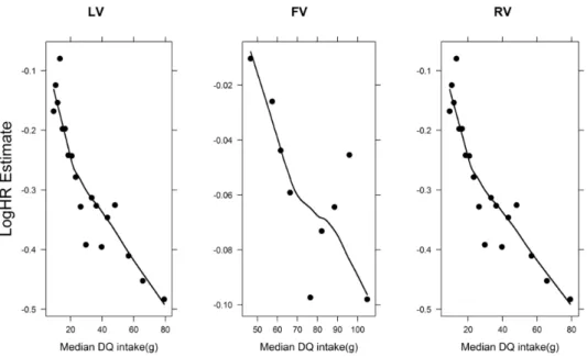
In each of these two forms of calibration models, we used the same set of covariates as in each part of the standard two-part calibration but with different parametric forms of the DQ intake as explained above. We conducted a backward elimination (α = 0.2) on each of these forms of regression calibration models to obtain their reduced forms. Subsequently, we used a Cox proportional hazard model in model (2.1) to study the association between usual intake of vegetable subgroups and all-cause mortality (Cox, 1972). The Cox proportional hazards model was stratified by centre and sex. To explore the form of relation between usual intake of each of the three vegetable subgroups and all-cause mortality in the Cox model, we plotted the log hazard ratio estimate against median intake in each DQ category (Sainani, 2009).
We used bootstrap procedure to compute correct standard error for the log hazard ratio estimate. The bootstrap approach accounts for the uncertainty in the calibration process. We used centre-stratified bootstrapping on the calibration sub-study. To each bootstrap sample, the main-study data was added and regression calibration model fitted to generate replicate versions of
E( |
R Q X
, )
for each subject in the entire EPIC cohort (Cassell, 2007). To each replicate data, the Cox model was fitted yielding an estimate of log hazard ratio with a standard error. The within-calibration and between-calibration variances were combined using Rubin’s formula to account for the uncertainty in the calibration process (Boshuizen et al., 2007; Geert Molenberghs, 2007; Rubin, 2004). The Rubin’s formula used to estimate the standard error for the log hazard ratio estimate is(
)
(
)
2 2 1 11
ˆ
1
1
ˆ
( )
SE(
)
1
1
m m i i i im
m
m
σ
2β
β
β β
Τ = =
=
+ +
−
−
∑
∑
, (2.6)29
where
σ
2Τ( )
β
is the total variance of the mean of log hazard ratio estimate from m calibrated samples,SE( )
β
ˆ
i is the within-calibration standard error, and(
)
2 11
ˆ
1
m i im
=β β
−
−
∑
is the between-calibration variance.We fitted a Cox proportional hazards model that ignores the measurement error in the DQ intake. This method is hereafter referred to as the naïve method. In the naïve method, the DQ intake measurements were used to study the association between usual intake of a vegetable subgroup and all-cause mortality.
2.3
Results
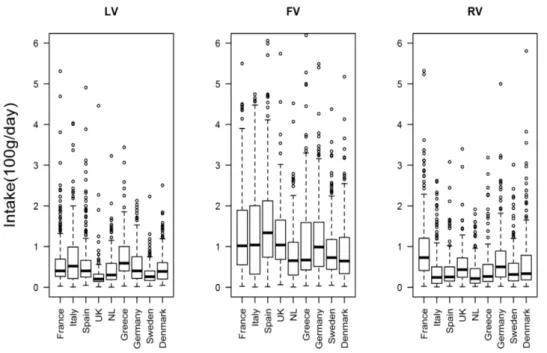
In Table 2.1, a high percentage of zeroes is shown in the 24-HDR intake for each of the three vegetable subgroups, especially for root vegetable subgroup in most of the participating countries. The rather high percentage of zeroes in the 24-HDR suggests that these subgroups of vegetables are not consumed daily by everyone. The Pearson correlation coefficient for each of the three vegetable subgroups in each of the participating countries, as measured with 24-HDR and DQ, were rather low but mostly statistically significant. The boxplots for the distribution of the consumed amount on consumption events as reported in the 24-HDR showed positive skewed distributions for these dietary intake variables (Figure 2.1). These exploratory findings suggested a need to properly handle the excess zeroes, to choose either a suitable distribution or a correct transformation for the consumed amount reported in the 24-HDR in building a calibration model.
30
Table 2.1: Country-specific summary measures for the percentage of zero intake
measurements reported on 24-HDR (% R=0, non-consumers) and Pearson Correlation (ρ) for intake as measured by 24-HDR and DQ for leafy vegetables, fruiting vegetables and root vegetables. EPIC Study, 1999-2000
Participating Countries Leafy vegetables Fruiting vegetables Root vegetables N % R=0 ρ % R=0 ρ % R=0 ρ France 4735 42.8 0.17 44.4 0.10 71.6 0.06 Italy 3961 59.3 0.16 37.6 0.15 79.6 0.11 Spain 3220 48.9 0.34 31.7 0.22 76.1 0.12 UK 1313 68.2 0.16 40.8 0.19 59.3 0.23 Netherlands 4545 70.5 0.10 48.7 0.21 82.0 0.14 Greece 2930 67.9 0.10 29.5 0.13 83.2 0.03ns Germany 4418 75.9 0.15 41.6 0.17 79.2 0.22 Sweden a 6132 70.5 0.19 34.9 0.24 67.2 0.17 Denmark 3918 77.4 0.09 41 0.21 61.8 0.40 Norway b1798 58.5 0.12
aN is 3132 instead of 6132 for leafy vegetables in Sweden because data from Umeå were
excluded from analysis based of the inclusion criteria in EPIC;
b
N refers to data for root vegetables only because data for Norway were excluded for leafy vegetable and fruit vegetable subgroups;
ns
means correlation is not statistically significant at α = 0.05, other correlation coefficients are highly significant with P < 0.0001.
31
Figure 2.1: The country-specific boxplots show the distribution of the consumed amount for those who reported consumption on the 24-HDR for leafy vegetables (LV), fruiting
vegetables (FV) and root vegetable (RV) subgroups in the EPIC study, 1992-2000.
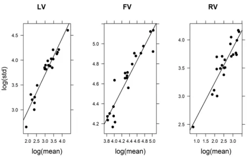
For each of the three vegetable subgroups, a linear trend is shown between the log of standard deviation and the log of the mean for the consumed amount reported in the 24-HDR (Figure 2.2). The linear trend is a clear evidence of a variance that increases with a mean (presence of heteroscedasticity). The slope (standard error) of least squares regression line fitted to the resulting scatterplots was estimated as 1.057 (0.085). For fruiting vegetables, the estimates were 0.994 (0.076). Likewise for root vegetables, the estimates were 1.021 (0.130). These slopes of the fitted lines were all close to the theoretical value of 1 for a GLM gamma model. Based on these exploratory findings, we chose a gamma GLM model for the consumed amount in part II of the two-part calibration model for each of the three vegetable subgroups.
The correlation between each of the three vegetable subgroups ranged from 0.06 to 0.12 with total energy and from -0.07 to 0.05 with alcohol, as measured with the DQ.
32
These low correlations suggest minimal contamination effect of measurement error on diet-disease association, hence justifying our choice not to adjust for measurement error also for these confounding variables.
Figure 2.2: Variance-mean relation for leafy vegetable intake (LV), fruiting vegetable intake (FV) and root vegetable intake (RV). The graph shows a least squares regression line fitted to the scatterplots of the logarithm of centre-specific standard deviation versus logarithm of centre-specific mean of the consumed amount for those who reported consumption on the 24HDR in the EPIC Study, 1992-2000. The approximately linear regression line suggests a variance that increases with the mean.
To explore the form of the DQ intake variable for the consumption probability part of the two-part calibration model, the loess curve fitted to the scatterplots of the empirical logit versus the mean intake in each DQ category showed a nonlinear relation between the logit of consumption as reported in the 24-HDR and the DQ intake (dotted lines in Figure 2.3). The GAM partial prediction plots showed similar behaviour. From the plausible set of parametric transformations for the DQ, here, square-root and logarithmic, we chose log-transformed DQ based on the AIC criterion for each model fitted to country-specific data. As a result, we fitted a logistic model with