Intergenerational
Risk Sharing in
Time-Consistent Funded
Pension Schemes
Ed Westerhout
CPB Discussion Paper
No 176
April 2011
Intergenerational Risk Sharing in
Time-Consistent Funded Pension Schemes
CPB Netherlands Bureau for Economic Policy Analysis Van Stolkweg 14
P.O. Box 80510
2508 GM The Hague, the Netherlands
Telephone +31 70 338 33 80
Telefax +31 70 338 33 50
Abstract in English
Intergenerational risk sharing by funded pension schemes may increase welfare in an ex ante sense. However, it also suffers from a time inconsistency problem. In particular, young generations may be unwilling to start participating in a pension scheme if this requires them to make huge transfers to older generations. This paper explores if limiting the transfers between generations can make a funded pension scheme time-consistent. The paper finds that this is possible indeed in a more or less realistic economic environment; it is not the case in general however. The form of the time-consistent scheme (how strong are the limits to transfers) is found to be very responsive to the economic environment. The time-consistent scheme offers lower welfare than the original time-inconsistent scheme, but higher welfare than a
defined-contribution scheme without any intergenerational risk sharing.
Key words: Public pensions, Time consistency, Optimal pension schemes
JEL code: H55
Abstract in Dutch
Intergenerationele risicodeling door pensioenfondsen kan welvaartsverhogend werken doordat risico's beter over generaties worden gespreid. Het creëert tegelijkertijd echter ook een tijdsconsistentieprobleem. Met name kunnen jonge generaties besluiten niet aan
pensioenregelingen deel te nemen als dit vereist dat ze hoge impliciete betalingen moeten doen aan oudere generaties. Dit paper onderzoekt of het mogelijk is pensioenregelingen
tijdsconsistent te maken door overdrachten tussen generaties te beperken. Het paper concludeert dat dit inderdaad mogelijk is in een meer of minder realistische omgeving; het is echter geen algemeen resultaat. De vorm van de tijdsconsistente regeling (hoe sterk zijn de beperkingen op overdrachten tussen generaties) blijkt sterk afhankelijk te zijn van de economische omgeving. Met de tijdsconsistente pensioenregeling wordt een minder hoog welvaartsniveau bereikt dan met de overeenkomstige tijdsinconsistente regeling. Het welvaartsniveau van de tijdsconsistente regeling is echter hoger dan dat van een individuele defined contribution regeling zonder enige vorm van risicodeling.
Intergenerational Risk Sharing in Time-Consistent Funded
Pension Schemes
Ed Westerhout
Abstract
Intergenerational risk sharing by funded pension schemes may increase welfare in an ex ante sense. However, it also suffers from a time inconsistency problem. In particular, young generations may be unwilling to start participating in a pension scheme if this requires them to make huge transfers to older generations. This paper explores if limiting the transfers between generations can make a funded pension scheme time-consistent. The paper finds that this is possible indeed in a more or less realistic economic environment; it is not the case in general however. The form of the time-consistent scheme (how strong are the limits to transfers) is found to be very responsive to the economic environment. The time-consistent scheme offers lower welfare than the original time-inconsistent scheme, but higher welfare than a
defined-contribution scheme without any intergenerational risk sharing.
Keywords: Public pensions, Time consistency, Optimal pension schemes
JEL Codes: H55
Affiliation: Ed Westerhout is affiliated with CPB Netherlands Bureau for Economic Policy Analysis and NETSPAR. The ideas expressed in this paper are strictly personal and do not necessarily reflect the views of CPB. Earlier versions of this paper were presented at the IIPF Conference, Cape Town, August 13-16 2009, at CPB, The Hague, January 12 2010, and at the
Netspar workshop, Amsterdam, January 27-29 2010. Thanks are due to Jan Bonenkamp, Lans Bovenberg, Casper van Ewijk, Hans Fehr, David Hollanders, Isidoro Mazza, Lex Meijdam, Ruud de Mooij, Peter Schotman and Siert-Jan Vos for useful comments and discussions. Thanks are due to André Nibbelink for excellent computational assistance.
1
Introduction
Defined benefit (DB) pension schemes share risks between generations. This raises aggregate welfare if households are risk averse (Gordon and Varian (1988), Shiller (1999), Ball and Mankiw (2007)) and if adverse general equilibrium effects on capital formation or labour supply do not dominate (Krueger and Kubler (2006), Sánchez-Marcos and Sánchez-Martín (2006), Bonenkamp and Westerhout (2010), Draperet al.(2011)).1Risk sharing schemes suffer from a time-consistency problem, however. Once a shock has materialized, some of the parties may find it unattractive to continue participation to the scheme. In particular, generations that are required to make transfers will in general not be willing to do so, even if they judged participation to the scheme as attractive before the uncertainty was resolved. If participation is voluntary, these generations will then decide to quit. If participation is obligatory, this route is blocked, but, in this case, these generations can vote with their feet. Indeed, they can reduce their labour market participation.2They can also emigrate to another firm, industry or country, depending on the coverage of the pension scheme in which they participate. They can also vote with their voice, for example by pleading for the introduction of an opting-out clause through the political process. As a consequence, it can be argued that, even if participation is mandatory, DB pension schemes are ultimately unsustainable.3
As such, the argument is incomplete, however. In particular, the opportunity costs of no longer being able to share the benefits from intergenerational risk sharing when they are old, may keep young generations from abandoning the contract. Hence, the welfare gain from risk sharing may act as a threshold for the transfers that can be imposed onto the younger
generations: only if these transfers exceed the money value of the threshold, will the young generations have an incentive to abandon the pension contract.4
The existence of a threshold has an important additional implication. In particular, it may be exploited to construct a scheme that avoids the discontinuity risk. The idea is to impose a limit to
1
Nishiyama and Smetters (2007) and Fehr and Habermann (2008) also focus on the tradeoff between the direct effects of risk sharing and the associated effects on economic behaviour. Different from our paper however, these papers focus on intragenerational rather than intergenerational risks.
2
This can be done in several ways. Workers can reduce their number of working hours or retire at some earlier date. Those who have not already entered the labour force can decide not to participate on the labour market or to postpone labour market entry. Moreover, workers and those outside the labour market can decide to become self-employed if the obligation to participate in the pension scheme does not apply to the self-employed. This is the case in the Netherlands, a country with which I am familiar.
3This result applies in case of a stable population structure. In the case of population ageing, which characterizes large parts of the western world, the risk that young generations opt out of the schemes may be larger.
4In general, there are several other reasons why young cohorts may favor a social security scheme. Examples are altruistic motives, dynamic efficiency and within-cohort redistribution. We will allow a role for these factors by introducing a catch-all variabledbelow. For a discussion of these motives, see Galasso and Profeta (2002).
the transfers from the young generations to the old generations that is equal to the money value of the threshold. This will then achieve that young generations will never find it beneficial to abandon the pension contract. In general, they will benefit from the contract; in the worst case, they will be indifferent between opting in and opting out. If we succeed to construct such a scheme, it may be expected to deliver lower welfare than the original scheme, but, unlike the original scheme, be time-consistent. If the scheme implies some risk sharing among generations, no matter how little, it will achieve higher welfare than the benchmark of an individual
defined-contribution scheme, in which there is no intergenerational risk sharing at all. However, a time-consistent scheme need not exist. The maximum transfer that young generations are required to make to the scheme determines not only the cost of participation, but also the benefit of participation upon changing the value of intergenerational risk sharing. In a rational expectations equilibrium, young generations are aware of the fact that limits to intergenerational transfers apply also when they have become old and will account for this in their decision-making. More specifically, if decreasing the maximum transfer that the young make to the old, reduces the future benefit from risk sharing more than the current cost, no time-consistent scheme will be found for which future benefit and current cost are equal for some level of maximum transfer.5Below, we will indeed encounter an example for which a non-trivial time-consistent scheme cannot be found.
We argue that the time-consistent scheme needs to obey a participation constraint for the young, but not for the old. The reason why is that opting out by the old differs on a crucial point with opting out by the young. Opting out by the old would mean that they abandon a (implicit) contract which they signed at some earlier date. Opting out by the young however means that they do not sign a contract that they consider unattractive in the first place. Supervisory policies suffice to achieve that signed contracts are respected, which means in this context that only the young will be allowed to opt out of the pension scheme.6
Can the old prevent a breakdown of the scheme through the political process (Gordon and Varian (1988))? This question relates to a large political-economy literature in which decisions on the contents of the pension scheme (and its continuation) are made in a voting process (Cooley and Soares (1999), Razinet al.(2002), Casamattaet al.(2005) and Cremeret al.
5
This may explain why Van Hemert (2005) fails to find a second-best scheme with positive transfers. In his analysis, transfers are one-sided, from the young to the old. An increase of the threshold rate of return below which no additional risk sharing will take place, may then reduce the gains from risk sharing in the retirement period more strongly than in our case, in which an increase of the threshold rate of return reduces both the transfers to and the transfers from the then young generation in the retirement period. The same may be true for Beetsmaet al.(2011), which also studies one-sided contracts.
6This restriction is also a necessary condition for an insurance contract. For if the old would have the possibility to opt out, no viable insurance contract would be possible: in all circumstances would one of the cohorts have an incentive not to respect the contract once the shock has materialized.
(2007)). Then, the weights attached to the interests of the young and the old determine what will be the final result. This paper argues that opting out can be achieved through other means as well, think of reducing labour market participation, shifting to some other industry or moving abroad. Therefore, we think that the incentives for young cohorts to leave the scheme should be given a larger weight than those for old cohorts. We take this to the extreme by disregarding completely the interests of the old in the process that describes the continuation of the scheme.
In the field of pensions, there is some earlier literature on the issue of discontinuity risk. Teulings and De Vries (2006) and Bovenberget al.(2007)reportthe discontinuity risk that corresponds with several degrees of intergenerational risk sharing. Gollier (2008) makes a step further: this paper explores a second-best scheme thatreducesthe discontinuity risk by a combination of investment policies, benefit policies and shareholder dividend policies. Beetsma
et al.(2011) explore pension contracts that limit the transfers from young to old generations in order to reduce the discontinuity risk. None of these paperseliminatesthe discontinuity risk completely however as the present paper does. In other parts of the economic literature, contracts that fully eliminate discontinuity risk have been studied before. Indeed, Thomas and Worrall (1988) studies wage contracts between workers and firms, Atkeson (1991) studies contracts between lenders and borrowers and Kocherlakota (1996) studies risk sharing contracts between different consumers.7
Our results are relevant for the current policy debate. Many countries consider to reform their pension schemes away from collective schemes with more defined benefit features towards individual schemes with more defined contribution features. Such a reform implies that the benefits from risk sharing will be lost. This paper points out that pension schemes can be reformed such that part of the intergenerational risk sharing and the associated benefits can be maintained. The proposed reform implies a reduction of risk sharing rather than a complete elimination of it.
The structure of the rest of the paper is as follows. Section 2 discusses the issue in general terms. It constructs a model in which households have 2-period lifes and in which a pension scheme shares risks between the two generations that overlap. Section 3 offers a numerical analysis to illustrate our findings. Section 4 presents a sensitivity analysis that shows the role of key parameters. Section 5 concludes.
7Each study has its own terminology. Thomas and Worrall (1988) talks about self-enforcing contracts, Atkeson (1991) talks about contracts that are individually rational and Kocherlakota (1996) talks about subgame-perfect allocations.
2
A model of risk sharing
Our model features overlapping generations of households and a pension fund. We describe them in turn. Before doing so however, we discuss the general properties of the model.
2.1
Outline of the model
We specify a model that contains only what is necessary to discuss our ideas. We thus adopt a small open economy framework with exogenous labor supply.8This leaves aside general equilibrium effects on labor and capital markets that are not crucial for a discussion of the time-consistency argument. There is only one risk factor, which is the return on a risky asset, the only financial asset that is available. We thus leave aside portfolio (re-)allocation effects and other risk factors, like labor productivity risk or demographic risk. Furthermore, we allow for only two generations in each period of time and include only two generations in our risk sharing scheme.
This modeling of the risk sharing scheme determines the nature of the model, which we consider to be static. Indeed, it implies that the model is without history. Immediately upon introducing a pension scheme, a new steady state is achieved. Our modeling of the risk sharing scheme also implies that it is suboptimal. Indeed, a scheme that would be chosen by a social planner would include all current and future generations into the risk sharing scheme (Ball and Mankiw (2007)). We have refrained from adopting such a first-best approach. Apart from changing the nature of the model from a static to a dynamic one, we doubt whether this approach would yield realistic results. Risk sharing would take an infinite number of years and current policies would still reflect shocks from many decades ago. Our model absorbs shocks within the unit period of the model, which we take to be about 30 years (each generation lives for two periods). Actually, we think 30 years may be unrealistically high, but surely not unrealistically low.
2.2
Households
Preferences are defined over consumption when young and when old,c1andc2. The rate of return on the only financial asset available,r, is stochastic and is drawn from an identical and independent distribution. The gross rate of return, 1+r, is strictly positive, thus the net rate of
8Bohn (2010) discusses the role of competitive labour markets in case of company pension funds. The pension scheme in our model should be interpreted as an institute that operates on a national scale, so that workers cannot escape increments in pension contributions by moving to a different firm.
return is strictly larger than -1. Hence, we assume the following:
Ut=u[c1,t,E˜t(c2,t+1)] +d (2.1)
c1,t=y−st−Π[(rt−Et−1(rt))st−1] (2.2)
c2,t+1=st(1+rt+1) +Π[(rt+1−Et(rt+1))st] (2.3) Equation (2.1) defines intertemporal utility for the generation born in periodt, which is assumed to be well-behaved. Period-tand earlier shocks have materialized before birth; period-t+1 shocks are unknown at that time. Therefore, equation (2.1) makes use of the expectations operator, dated in periodt. The expectations operator in (2.1) refers to a certainty-equivalent expectation (Epstein and Zin (1989)), which we will elaborate below. We use a tilde to distinguish this expectations operator from the standard expectations operator. Equations (2.2) and (2.3) make up the budget constraint. Here,ydenotes exogenous labour income ands
denotes savings.
Equations (2.2) and (2.3) include a risk sharing functionΠ, which describes the transfer from the young to the old generation through the pension scheme. The risk sharing function has as argument(rt−Et−1(rt))st−1, which is the unexpected part of the return on saving times the amount of saving, or, more compactly, the unexpected capital income of the old. Given that we assume the rate of return on savings to be i.i.d., we will useE(r)as a shorthand notation for
Et−1(rt)in the following. The risk sharing function differs for the three cases that this paper will explore: the defined-contribution case, the time-inconsistent hybrid case and the time-consistent hybrid case. We will discuss the function in detail below.
The variabledin equation (2.1) denotes the value of participation in a pension scheme that shares risks between generations. Indeed,d takes a zero or positive value in the two public schemes, whereas it has zero value in the individual DC scheme. The variabled reflects a preference for solidarity. It assumes that people are happy to participate in a public pension scheme that features solidarity between generations by transferring risks borne initially by some generation to other generations. This may be interpreted as altruism or inequity aversion, aspects that are strongly supported by empirical evidence (Fehr and Schmidt (1999).
Should we interpret the individual DC scheme as individual savings held in the form of bank accounts,dcould be given a wider interpretation. For example, it could reflect the assumption that pension funds are better investors than individual households in the sense that the former reap higher average returns or less variable returns on their savings. Henceforth, we will adhere to the interpretation of the individual DC scheme as a pension scheme that invests solely for the purposes of a specific generation and that does not engage in intergenerational transfers however.
2.3
Pension transfer schemes
We distinguish between three different types of pension schemes: a pure defined-contribution (DC) scheme and two types of hybrid schemes, a time-inconsistent one and a time-consistent one. The latter two schemes are hybrid in the sense that they are in between pure defined-benefit (DB) and pure DC schemes. To make the three schemes comparable, we assume that they levy the same average premiums upon working households. They differ only in the corresponding risk sharing schemes that apply to pension contributions and benefits.
The level of pension premiums can be pinned down at several levels. A natural option is to set premiums at the level that maximizes household welfare in the DC scheme. Formally,stis then determined by the first-order condition∂E˜t−1(Ut,dc)/∂st=0, where we use subscriptdcto refer to the DC case. Note that a period-tshock in the rate of return does not affect welfare of the household born in periodt: not directly, as households enter economic life without financial wealth, nor indirectly, as the DC scheme does not feature any intergenerational transfers with the generation born in periodt−1. Hence, the above first-order condition is equivalent to
∂Ut,dc/∂st=0.
The DC scheme is defined as the scheme without any intergenerational transfers:
Πdc[(rt−E(r))st−1] =0 (2.4)
In the case of a time-inconsistent hybrid scheme, we specify redistributive transfers as proportional to the deviation of the contemporaneous rate of return from its expected value,
Πti[(rt−E(r))st−1] =π(rt−E(r))st−1 (2.5) where subscripttiis used to refer to the time-inconsistent hybrid scheme.
Combining this equation with that for period-2 consumption, equation (2.3), gives an expression for the rate of return on pension saving in the time-inconsistent hybrid scheme: 1+rt+1+π(rt+1−E(r)). The value of the risk sharing parameterπ determines the nature of the
pension scheme. Ifπ equals -1, we have that the rate of return on pension saving is
non-stochastic. We then have a pure DB scheme, in which the pension benefit is completely unrelated to the capital market rate of return. Ifπ equals 0, the scheme coincides with the DC
scheme. If−1<π<0, the pension scheme is a hybrid case, in between the cases of a pure DB
and a pure DC scheme.
In the time-consistent case, the redistributive function is more complex:
Πtc[(rt−E(r))st−1] =π(max[rˆt,min[rt,r¯t]]−E(r))st−1 (2.6) where subscripttcis used to refer to the time-consistent hybrid scheme.
The latter formula includes a max-min function of the contemporaneous rate of return on savings and threshold returns ˆrtand ¯rt, to be defined later, rather than the contemporaneous rate of return itself. This limits the redistributive transfers between the young and the old: transfers from the young to the old cannot exceedπ(E(r)−rˆt)st−1; transfers to the young cannot exceed
π(r¯t−E(r))st−1.
The static nature of our model implies that not onlyE(r)is time-invariant. Also, the level of saving and the two threshold rates of return are constant through time. Hence, we will denote these ass, ˆrand ¯rrespectively, thus omitting the time index, in the following.
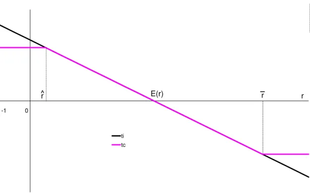
Figure 2.1 illustrates. It depicts the transfers from the young to the old through the pension scheme in the case of a time-inconsistent and time-consistent pension scheme. The
time-inconsistent pension scheme implies intergenerational transfers that are proportional with
rt−E(r). The time-consistent pension scheme restricts the size of intergenerational transfers both on the downside and the upside. Figure 2.2 displays the consequences for second-period consumption. The curve that refers to the time-inconsistent case is flatter than that corresponding to the DC case, reflecting the risk sharing in the former case. This assumes−1<π <0. If π =−1, the consumption curve for the time-inconsistent scheme would be flat and ifπ=0, it
would have the same slope as the conusmption curve for the individual DC scheme. In the time-consistent case, the curve is also flatter, but only on the domain ˆr<rt<r¯. Outside this domain, the curves of the time-consistent scheme and of the DC scheme move parallel to one another. This reflects that forrt<rˆandrt>r¯, the time-consistent pension scheme provides no risk sharing at the margin.
The max-min function in equation (2.6) truncates the distribution of the rate of return twice: atrt=rˆand atrt=r¯. In our discussion of the time-consistent pension scheme below, we will explain that the participation decision of the young cohort determines the value of ˆr. The value of ¯rrelates to the value of ˆr: ¯rwill be chosen such that expected transfers between the young and the old are zero.
Note that any scheme with−1≤π<0 achieves risk sharing between the young and old
generation. We let the pension fund chooseπ such that it maximizes the expected lifetime utility
of the generation that is born at the time at which the pension scheme is introduced. This approach differs somewhat from the approach of maximizing a social welfare function, as pursued by for example Gollier (2008) and Bohn (2009). The advantage of our approach is that it allows us to establish whether the introduction of a pension scheme is Pareto improving. This criterion is stronger than that of a potential Pareto improvement, which results from adopting a social welfare approach.
Our approach is not necessarily the most realistic one, as it neglects the political
Figure 2.1 Risk-sharing transfers in the time-inconsistent and time-consistent pension scheme ti tc r E(r) r r -1 0 Δ
benchmark that can be used to illustrate the effects of discontinuity risk. Moreover, it is sufficiently general to capture a large number of real-world pension schemes in between pure defined-benefit and defined-contribution.
Intertemporal utility as defined in equation (2.1) is an ex post measure. For welfare analysis, we also define its ex ante counterpart, which is the (certainty-equivalent) expectation of
intertemporal utility over all possible realizations ofrt:
Vt=E˜t−1(Ut) (2.7)
It is now time to characterize the time-inconsistent and time-consistent scheme. We start with the former.
2.4
The optimal time-inconsistent hybrid scheme
We define the optimal time-inconsistent scheme as the scheme with that value ofπ, denotedπ∗,
that maximizes welfareVas defined in equation (2.7).π∗follows from elaborating the
corresponding first-order condition,
Figure 2.2 Period-2 consumption in the three equilibria dc ti tc r -1 0 ƌ Δ ;ƌͿ ͺƌ
Substitution ofπ∗into the expression forVt,tiyieldsVt∗,ti,i.e.welfare under the optimal time-inconsistent hybrid scheme.
2.5
The optimal time-consistent hybrid scheme
The optimal time-inconsistent scheme takes over the slope of its risk sharing scheme from the optimal time-consistent scheme. This may be suboptimal. Numerical problems hinder an extension to different slopes, however. Moreover, such an extension is not really necessary for our purpose of showing that a pension scheme can be made time-consistent.
Specific to the time-consistent scheme is that it truncates the transfer function. It does so at two sides, at rates of return ˆrand ¯r. The truncation at the downside of the rate-of-return distribution is due to the participation constraint which we will elaborate below. Restricting risk sharing at the upside goes along with risk sharing at the downside such as to ensure that average transfers in the time-consistent scheme are zero. Allowing non-zero average transfers would imply ex ante redistribution between the two generations.9This would bring in a PAYG element in the time-consistent scheme and would make it impossible to attribute differences between the
9The difference between ex ante redistribution and risk sharing is that risk sharing between generations is conditional on the occurrence of a shock. Ex ante redistribution occurs irrespective the occurrence of a shock.
time-inconsistent scheme and the time-consistent scheme solely to their risk characteristics. Formally,
E(max[rˆ,min[r,r¯]]) =E(r) (2.9)
This equation implicity solves for ¯ras a function of ˆr.
The participation constraint specifies ˆr, the rate of return at which the rate-of-return distribution will be truncated at the downside. We find the value of ˆrby specifying that the participant will be indifferent between participating in the pension scheme and staying out of the scheme ifrt=rˆ, recognizing that the same truncation will apply to the rate-of-return distribution in periodt+1. Forrtlower than ˆr, transfers are at their maximum andUt,tc=Ut,dc. Forrt higher than ˆr, transfers to the old cohort are lower (and possibly negative) andUt,tc>Ut,dc. This scheme is time-consistent as the participation constraint is obeyed in all states of nature (all values ofrt): putting ˆrat a lower value would violate the constraint for at least some values ofrt. The scheme is optimal as it minimizes the probability that the constraint is binding: puttingrtat a higher value would restrict intergenerational risk sharing too much and therefore yield lower ex ante utility. In the general case in which -1< ˆr<E(r), both the case in which the participation constraint is binding and the case in which it is not have strictly positive probability.
Formally, the participation constraint gives the value of ˆrthat ensures that participation in the time-consistent scheme delivers as much utility as staying out of the pension scheme if the period-trate of return on saving equals ˆr,
Ut,tc(rt,rˆ,r¯(rˆ)) =Ut,dc rt=rˆ (2.10) where I have made explicit thatUt,tcis a function ofrt, the realization of the period-trate of return on savings, and ˆrand ¯r, the threshold rates of return.
Having solved for ˆr, we can substitute it into the expression forVt,tc, which gives usVt∗,tc. We assume thatUt,ti−Ut,dc<0 forrt=-1, the worst possible state. If this were not true, participation in the time-inconsistent pension scheme would be beneficial for all values ofrtand the time-inconsistent scheme would be viable. Second, we assume thatUt,ti−Ut,dc>0 for
rt=E(r). This is a quite weak assumption, which reflects the gains from intergenerational risk sharing.
Despite these assumptions, a solution to the participation equation may not exist. As the participant is rational, he recognizes that changing the maximum of transfers to the old generation affects not only the current cost of participation, but also the future benefit of participation upon changing the value of intergenerational risk sharing. If, starting at a rate of return for which participation in the pension scheme gives lower utility than the fall back of staying out, decreasing the maximum transfer that the young make to the old reduces the future benefit more than the current cost, no time-consistent scheme will be found.
In the simulations presented in this paper that do find a solution for the optimal
time-consistent scheme, the rate-of-return distribution is separated in three different regions, one in which the participation constraint is binding and transfers by the young are at their maximum, one in which transfers by the young are at their (negative) minimum and one in which transfers are in between their minimum and maximum (see also Figure 2.1).
2.6
Welfare assessment
Our policy experiment is extremely simple. Initially, we have an individual DC scheme. At time
tthen, nothing changes (the DC scheme continues) or a time-inconsistent hybrid scheme is introduced or a time-consistent hybrid scheme is introduced. Furthermore, from now on we will use the term time-(in-)consistent hybrid scheme to denote the optimal time-(in-)consistent hybrid scheme; suboptimal hybrid schemes will not be studied. In case a time-(in-)consistent hybrid scheme is introduced, the policy change was not announced before, which rules out any anticipation effects. The model is such that it reaches a steady state immediately upon changing the pension scheme. Periodst+i i=1,2, ..are thus equivalent with periodt. Generations affected by the policy change are the generation that is old at the time of the policy change, the generation who is young at the time of the policy change and the generations born in later time periods. We call the former generation the transitional generation and all other generations steady-state generations.
We rank the DC scheme, the optimal time-inconsistent hybrid scheme and the optimal time-consistent hybrid scheme by their (ex ante) welfare measures,i.e. Vt−j,dc,Vt∗−j,tiand
Vt∗−j,tc. Here, j=0,1, withj=0 referring to steady-state generations and j=1 referring to the transitional generation. To enable a meaningful interpretation, we also calculate the
corresponding consumption-equivalent welfare changes. The consumption-equivalent welfare change measures by how much percent a generation’s consumption (in both periods and in all states of the world) in the DC case would need to change to obtain the same level of welfare as in the (time-inconsistent or time-consistent) case with a pension scheme. We will denote the consumption-equivalent welfare change asCVt−j,tiandCVt−j,tc j=0,1 for the
time-inconsistent and time-consistent case respectively.
A complicating factor arises in case of a non-zero preference for public schemes (d=0). The calculated welfare effects then mix two things: the gains from risk sharing and the utility value of the preference for public schemes. In order to extract the welfare gain that is due to intergenerational risk sharing only, we also calculate consumption-equivalent welfare changes relative to a hypothetical DC scheme in which households attach the same utility to participation as they do in the two public schemes. We use tildes to denote the corresponding
consumption-equivalent welfare changes: ˜CVt−j,tiand ˜CVt−j,tc j=0,1. Obviously, in case
d=0, the latter coincide with the original welfare measuresCVt−j,tiandCVt−j,tc. Importantly, the welfare effect of the transitional generation dominates that of the
steady-state generations. Indeed, the steady-state generations share risks both when young and when old with the other generation that is alive at that time. The transitional generation,i.e.the generation who is old at the time the pension scheme is introduced, will engage in
intergenerational risk sharing only when old. Hence, the transitional generation will always be more positively affected by the introduction of the pension scheme than the steady-state generations. Indeed, like the steady-state generations, the transitional generation benefits from more stable old-age consumption, but, unlike the steady-state generations, does not suffer from less stable working-age consumption. To evaluate whether the introduction of a pension scheme will constitute a Pareto improvement, we can therefore abstract from the welfare effect upon the transitional generation. Indeed, if the introduction of the pension scheme increases the welfare of the generation born att, all generations enjoy a welfare gain and the policy change constitutes a Pareto improvement.
3
A numerical assessment of the gains from risk sharing
This section presents a benchmark simulation that illustrates the ideas developed in the previous section and that provides insight into the order of magnitude of likely effects. Subsection 3.1 lists the assumptions we make on preferences, the economic environment and parameter values. Section 3.2 discusses the results for the benchmark case.
3.1
Assumptions for the benchmark case
There is one risk factor: the rate of return on savings. Preferences, defined over consumption, are of the recursive utility type: they feature an elasticity of intertemporal substitution and a
coefficient of relative risk aversion that are both constant but not necessarily each other’s reciprocal (Epstein and Zin (1989)). Hence, we assume the following:
u[c1,t,c2,t+1] = c1−θ 1,t + 1 1+δ c1−θ 2,t+1 1−1 θ (3.1) Ut=u[c1,t,E˜t(c2,t+1)] +d= c1−θ 1,t + 1 1+δ [Et(c12−,t+σ1)] 1−θ 1−σ 1−1θ +d (3.2) Vt=E˜t−1(Ut) = Et−1 c1−θ 1,t + 1 1+δ [Et(c12−,t+σ1)] 1−θ 1−σ 1−1 θ +d !1−σ 1 1−σ (3.3)
where 1/θdenotes the elasticity of intertemporal substitution,σ denotes the coefficient of
relative risk aversion andδdenotes the rate of time preference.
We adopt Epstein-Zin preferences since they allow us to disentangle the aversion of the consumer for risk and for intertemporal fluctuations; these two aspects of consumer preferences are described by two different parameters,σandθrespectively. The case where preferences are
additively separable is a special case of these more general preferences; it results when we imposeσ=θ(in this special case, the general expectations operator ˜Ecoincides with the
standard expectations operatorE).
Our benchmark calculation puts the intertemporal elasticity of substitution to 0.5 and the coefficient of relative risk aversion to 10. This is in line with the literature that finds the intertemporal elasticity of substitution to be close to zero and the coefficient of relative risk aversion to be much larger than one. Estimates of both parameters exhibit a large variety in the literature however, so we will perform a sensitivity analysis to find out how important are the values of these parameters for our results.
The rate of time preference is taken to be 4.74. This implies an annual rate of 6%. Sensitivity simulations reported on below show that the relevance of the numerical value of this parameter is quite small. Altruism is absent in our benchmark simulation:d=0. Finally, labour income,y, a scaling variable, takes a value of 100.
We assume that the return on savings is lognormally distributed. This assumption is quite common, although a distribution with thicker tails would provide a better match with the data.10 The lognormal distribution is quite handy when it comes to transforming an annual distribution into the 30-year distribution that we use in our analysis. It is also handy to relate the two threshold rates of return to one another.11
In particular, the log of the gross rate of return on savings follows a normal distribution with mean 1.202 and variance 0.225. This corresponds to the assumption that the annual rate of return on savings has a mean of 4.48% and a standard deviation of 9.06%, that the unit period of our model covers 30 years and that the return on savings follows a lognormal distribution that does not change over time. The figure for the standard deviation is taken from Campbell and Viceira (2002), after correction for the fact that we assume savings to consist of riskless bonds and risky equity in equal amounts. The figure for the mean is also based on Campbell and Viceira (2002), but corrects for the fact that in general the historical excess return can deviate strongly from the
10One reason for this may be rare disasters (Barro (2006)).
11Equation (2.9) specifies the condition that average transfers are zero in the time-consistent scheme:
E(max[rˆ,min[r,r¯]]) =E(r). If the rate of return on savings is lognormally distributed, this condition can be elaborated as
F((log(1+r¯)−µr)/σr)−F((log(1+rˆ)−µr)/σr) =F(((log(1+r¯)−µr)/σr)−σr)−F(((log(1+rˆ)−µr)/σr)−σr),
whereF(.)denotes the standard normal distribution function andµrandσrrefer to the mean and standard deviation of log(1+r)respectively.
equity premium. Fama and French (2002) present two calculations of the difference between the two concepts. The average of their estimates of the difference between the historical excess return and the equity premium is 4%-point. In order to give equal support to the two strands, we reduce Campbell and Viceira’s (2002) estimate with half the difference as calculated by Fama and French. Hence, we reduce Campbell and Viceira’s (2002) average rate of return on equity, 8.85%, with 2%-points, giving an estimate equal to 6.85%. Recalling that the riskless rate of return equals 2.11% and that savings are made up of riskless bonds and risky equity in equal amounts, we calculate the average annual portfolio rate of return to be
1/2*(2.11%+6.85%)=4.48%.
Our stochastic simulation takes 200 draws for each of the two stochastic variables, giving 40,000 runs in total. In order to reduce sample bias, we make two corrections to the draws. First, we add a factor to all sample elements such that the sample mean becomes equal to the
theoretical mean, which coincides with the sample mean in an asymptotically large sample. Second, we multiply all sample elements in deviation from their theoretical mean with a factor that brings equality between the sample variance and the theoretical variance, which, similar to the theoretical mean, applies in the asymptotic case. As sample elements we take the log return realizations to avoid that these corrections would render one or more rate of return data negative (see Poterba (2004) for a similar procedure).
3.2
Results for the benchmark case
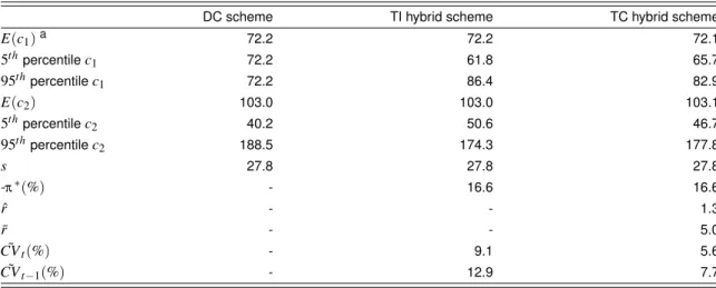
Table 3.1 summarizes our results for the benchmark case. The first column shows results for the DC scheme. Pension savings equal 27.8 (27.8 percent of a wage income of 100), so that first-period consumption has a value of 72.2. Second-period consumption in the defined-contribution scheme is stochastic. On average, it equals 103.0, but there is huge variation around this average value. Indeed, Table 3.1 shows that the 5th and 95th percentiles deviate strongly from the average value (40.2 and 188.5 respectively).
The second column of Table 3.1 displays the time-inconsistent (TI) hybrid scheme. This scheme features risk sharing between the young and old generation. Indeed, the
time-inconsistent hybrid pension scheme shifts risk away from the period of retirement towards the period of labor market participation. This is seen in the figures for the 5thpercentile and 95th percentile of first-period consumption; equal in the DC scheme and strongly different in the TI scheme. It is also seen in the corresponding figures for second-period consumption; the 5thand 95thpercentiles of second-period consumption deviate substantially less from the mean of the distribution in the TI case.
Table 3.1 The three pension schemes in the benchmark case
DC scheme TI hybrid scheme TC hybrid scheme
E(c1)a 72.2 72.2 72.1 5thpercentilec1 72.2 61.8 65.7 95thpercentilec1 72.2 86.4 82.9 E(c2) 103.0 103.0 103.1 5thpercentilec2 40.2 50.6 46.7 95thpercentilec2 188.5 174.3 177.8 s 27.8 27.8 27.8 -π∗(%) - 16.6 16.6 ˆ r - - 1.3 ¯ r - - 5.0 ˜ CVt(%) - 9.1 5.6 ˜ CVt−1(%) - 12.9 7.7
a We omit the time subscript unless this could be confusing.
the TI scheme shifts about a sixth of the capital income risk for the old in the DC scheme towards the younger cohort. Even in the TI scheme, the elderly thus bear more risk than the youngsters. That the two do not share equally the capital income risk in the economy is due to the fact that in our model, risk aversion with regard to second-period consumption is lower than that with regard to first-period consumption on account of time preference.
The consumption equivalent of the welfare gain from a move from the DC scheme to the time-inconsistent hybrid scheme equals 9.1%. The welfare gain for the transitional generation is higher, as explained above: it is calculated as 12.9%.
As will be clear by now, the problem with the time-inconsistent scheme is that utility from an ex post perspective may be lower than utility in the fall-back option, which here is the DC scheme. We can calculate a threshold rate of return at which the time-inconsistent scheme and the DC scheme are equivalent from an ex post perspective. We now writeUt,tiexplicitly as a function ofrt, note thatUt,dcis independent ofrt and denote the threshold rate of return as ˚r. We can then derive a value for ˚rfrom the following condition:
Ut,dc=Ut,ti(r˚) (3.4)
For the benchmark case, we can calculate that ˚r=0.6. To this corresponds a probability of 5.6%. Can we now find a time-consistent scheme that eliminates this discontinuity risk?
The third column of Table 3.1 answers this question in the affirmative. It indicates that the optimal time-consistent scheme features threshold rates of return, ˆrand ¯r, that equal 1.3 and 5.0 respectively. Note that ˆris higher than ˚r. This is intuitive. Atrt=r˚,Ut,tcwill be less thanUt,ti (andUt,dc, asUt,tiandUt,dcare equal by definition) as the time-consistent scheme yields less risk sharing than the time-inconsistent scheme in the second period of life. ˆris defined as the value
ofrtfor whichUt,tcequalsUt,dc. Thus,Ut,tcmust be raised and this is achieved by restricting further the maximum transfer imposed on the young generation. Hence, ˆrmust be higher than ˚r.
Hence, the transfer scheme of the time-consistent pension scheme is flat for rates of return in between -1.0 and 1.3 and for rates of return higher than 5.0. To ease interpretation, this
corresponds with annual rates of return of 2.8%((1+1.3)1/30−1)and 6.2%((1+5.0)1/30−1) respectively.
One may recall that we have chosen to construct our time-consistent pension scheme such that it does not entail ex ante redistribution between the generations. Hence, average
consumption in the two periods should be equal for the two types of hybrid pension schemes. Table 3.1 shows that this is not completely true in the case of the TC hybrid scheme, although the differences are small. The reason for this is small sample size. The differences are such small that we consider our sample as sufficiently large.
The TC case compromises the DC case and the TI case in terms of the spread of first- and second-period consumption. The 5th and 95thpercentiles of first-period consumption are in between their counterparts of the DC case and the TI case; the same holds true with respect to the corresponding percentiles of second-period consumption. The frequency distributions of
c2,t+1have a similar shape in the three schemes, with the DC scheme featuring the highest degree of dispersion and the TI scheme the lowest. As regardsc1,t, the frequency distributions are different however. In the DC case, the frequency distribution boils down to one spike; absent intergenerational transfers,c1,tis non-stochastic. The time-inconsistent case features a sort of continuous distribution. As a result,c1,tin the time-consistent case features a distribution that combines two spikes with a sort of continuous distribution in between. This reflects thatc1,twill deviate from its mean because of intergenerational transfers and that these transfers feature a lower and upper bound. The two spikes reflect the bounds and the distribution in between the spikes reflects the unbounded transfers.
The time-consistent scheme adds less to welfare than the time-inconsistent scheme. Indeed, the consumption equivalent of the welfare gain (corrected for the participation preferenced) is now 5.6%, compared with 9.1% in the time-inconsistent case. Similarly, the consumption equivalent of the welfare gain for the transitional generation is now 7.7% and 12.9% in the time-inconsistent case.
How do the calculated welfare gains in the time-inconsistent case relate to those of earlier research? A number of papers have reported effects for steady-state generations. Cuiet al.
(2011) presents calculations of the welfare gain due to intergenerational risk sharing in the range 2-4%. Bonenkamp and Westerhout (2010) assess the welfare gain from risk sharing to be an order of magnitude higher: 7.1%. Similarly, Bovenberget al.(2007) calculates a welfare gain of 8.3%. Gollier (2008) presents a much larger effect: 19%. The differences in the results of the
different papers seem to be due to different modelling assumptions (two-period versus multi-period lives, risk sharing between two versus an infinite number of generations, consumption versus terminal wealth as argument of the utility function, two financial assets versus one financial asset), different parameter values (as regards the coefficient of risk aversion, the mean and standard deviation of the equity rate of return) and the approach to calculate welfare effects (an overlapping-generations approach versus a representative-agent approach). The range of results is thus fairly wide; our results are somewhere in the middle of this range. The consumption equivalents of the utility gains in the time-consistent case are little smaller than their counterparts in the time-inconsistent case: 5.6% compared with 9.1% for the
steady-state generations and 7.7% compared with 12.9% for the transitional generation. The elimination of discontinuity risk thus reduces the scope for intergenerational risk sharing, but does not eliminate it. The effects in Gollier (2008) are more outspoken: there, the move from a first-best scheme to a second-best scheme about halves the welfare gain from intergenerational risk sharing.
4
Alternative simulations
This section presents two sets of alternative simulations. The first set varies the value ofd. The second set of alternative simulations explores the role of values of parameters that describe preferences and parameters that describe the economic environment.
4.1
The role of altruism
In order to find out the role of altruism, we run simulations with different values ford. The other parameters take the same values as in the benchmark case.
Table 4.1 Analysis of the effect of altruism
Number d -π∗(%) CV˜ t,ti(%) CV˜ t−1,ti(%) rˆ r¯ CV˜ t,tc(%) CV˜ t−1,tc(%)
BM 0.0 16.6 9.1 12.9 1.3 5.0 5.6 7.7
1 1.0 16.6 9.1 12.9 0.6 7.9 7.2 10.5
2 3.0 16.6 9.1 12.9 -0.4 20.6 9.1 12.9
The pattern that emerges from the simulations is clear. Increasing the value fordmakes the public pension scheme more attractive and thus decreases the discontinuity risk. As a
consequence, the time-consistent pension scheme can decrease the value for ˆrand increase that of ¯r, thus enlarging the scope for risk sharing. This increases the welfare gains that the
time-consistent scheme achieves as compared with the individual DC scheme, both for steady-state and transitional generations.
A value fordof 3.0 is already sufficient to let the problem of discontinuity risk disappear. Indeed, ˆris chosen extremely low and ¯rextremely high. The welfare gains to steady-state and transitional generations are approximately the same as the welfare gains in the time-inconsistent case.
4.2
Sensitivity analysis
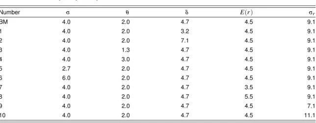
In order to find out how the results of the previous section relate to our assumptions on the values of key parameters, we conduct a sensitivity analysis. In particular, we simulate economies with higher and lower values for the parameters that describe preferences (the coefficient of relative risk aversion, the elasticity of intertemporal substitution and the rate of time preference) and for the parameters that describe the economic environment (the mean and the volatility of the rate of return on saving). Table 4.1 reports on the input of the simulations, Table 4.2 on the output.
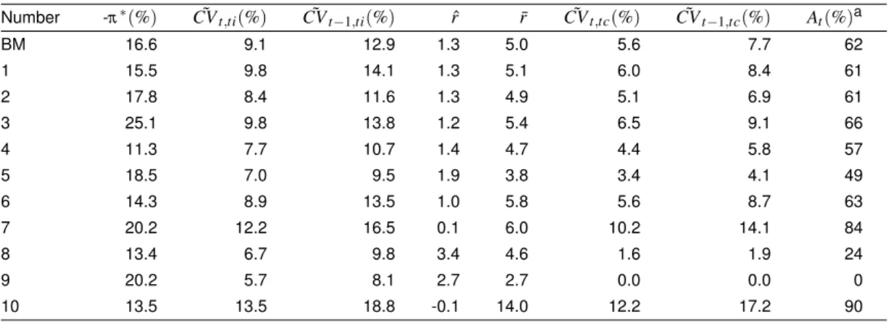
A few observations can be made. First, the range of welfare gains is large, both for the time-inconsistent case and the time-consistent case. In case of the time-consistent pension scheme, the welfare effects for steady-state generations range from zero to 12.2%. Second, the welfare gain achieved by a time-consistent scheme is a sizeable fraction of the gain that the corresponding time-inconsistent scheme brings about: for steady-state generations, this fraction amounts to 62% in the benchmark case with much lower and higher values in some of the other simulations.
Thirdly, variations in the coefficient of relative risk aversion exercise substantial effects. The simulations that adopt values for the coefficient of relative risk aversion of 6.7 and 15 achieve corrected consumption-equivalent welfare gains for steady-state generations that equal 3.4% and 5.6% respectively. The relation between risk aversion and the welfare gain from a
time-consistent pension scheme is clearly positive on two accounts. First, a higher degree of risk aversion directly increases the utility gain from a better risk allocation. Second, an indirect effect reinforces this direct effect: a higher risk aversion softens the participation constraint, which induces the pension fund to organize more risk sharing in the time-consistent scheme. Krueger and Kubler (2006) also derive that the welfare gain from pension schemes relates positively to the degree of risk aversion. Yet, the result is not general however. In particular, in a model with an endogenous portfolio choice, higher risk aversion may induce households to choose more conservative portfolios, thereby reducing the welfare gains from risk sharing (Gollier (2008), Bonenkamp and Westerhout (2010) and Cuiet al.(2011)).
larger effects than those of variations in the degree of risk aversion. A higher mean rate of return on savings reduces the welfare gain from a pension scheme. A higher mean rate of return raises consumption in the case of a DC scheme; a given gain in consumption in absolute terms then counts less in relative terms. A higher standard deviation of the rate of return on savings has the opposite effect. It reduces consumption in the case of a DC scheme. A given gain in
consumption in absolute terms then counts more in relative terms. Interestingly, the case of a lower volatility is extreme in the sense that no non-trivial time-consistent pension scheme can be found. Intuitively, the gains from risk sharing are too small to compensate young generations for potentially large payments in the first period of their lives. The only scheme that obeys the participation constraint is then one that coincides with a DC scheme and which offers no risk sharing at all ( ˆrand ¯rhave converged to a single value). Simulations (not shown) in which we took a much more conservative value for the coefficient of risk aversion, namely 4, yielded the same result. Hence, the result that a time-consistent scheme may not exist is robust and will arise when the gains from risk sharing are large, on account of low volatility or low risk aversion.
Fifthly, the effects of variations in the rate of time preference and the elasticity of
intertemporal substitution are small. Although the effects are clearly non-zero, they are an order of magnitude smaller than the effects that are due to changing risk aversion or the mean or standard deviation of the rate of return on savings.
Table 4.2 Sensitivity analysis: input
Number σ θ δ E(r) σr BM 4.0 2.0 4.7 4.5 9.1 1 4.0 2.0 3.2 4.5 9.1 2 4.0 2.0 7.1 4.5 9.1 3 4.0 1.3 4.7 4.5 9.1 4 4.0 3.0 4.7 4.5 9.1 5 2.7 2.0 4.7 4.5 9.1 6 6.0 2.0 4.7 4.5 9.1 7 4.0 2.0 4.7 3.5 9.1 8 4.0 2.0 4.7 5.5 9.1 9 4.0 2.0 4.7 4.5 7.1 10 4.0 2.0 4.7 4.5 11.1
5
Concluding remarks
This paper started from the observation that participation in a pension scheme that shares risks between generations may be unattractive, even if the scheme increases efficiency in an ex ante sense. Indeed, welfare of some future generation may decrease in states of nature that are bad as
Table 4.3 Sensitivity analysis: output Number -π∗(%) CV˜ t,ti(%) CV˜ t−1,ti(%) rˆ r¯ CV˜ t,tc(%) CV˜ t−1,tc(%) At(%)a BM 16.6 9.1 12.9 1.3 5.0 5.6 7.7 62 1 15.5 9.8 14.1 1.3 5.1 6.0 8.4 61 2 17.8 8.4 11.6 1.3 4.9 5.1 6.9 61 3 25.1 9.8 13.8 1.2 5.4 6.5 9.1 66 4 11.3 7.7 10.7 1.4 4.7 4.4 5.8 57 5 18.5 7.0 9.5 1.9 3.8 3.4 4.1 49 6 14.3 8.9 13.5 1.0 5.8 5.6 8.7 63 7 20.2 12.2 16.5 0.1 6.0 10.2 14.1 84 8 13.4 6.7 9.8 3.4 4.6 1.6 1.9 24 9 20.2 5.7 8.1 2.7 2.7 0.0 0.0 0 10 13.5 13.5 18.8 -0.1 14.0 12.2 17.2 90 aA tdenotesCV˜ t,tc/CV˜ t,ti.
seen from an ex post perspective. The central result of this paper is that generally such welfare losses can be eliminated by limiting the transfers between generations. As some risk sharing between generations is maintained, the introduction of a time-consistent scheme that avoids ex post welfare losses entails a Pareto improvement.
As a consequence, the government does not need to oblige people to participate in the pension scheme. It is important to provide two caveats in this respect, however. First, our paper has assumed like most of the literature that people are forward looking and do not suffer from short-sightedness. If people are myopic however, they may fail to recognize the benefits from future risk sharing and hence decide not to participate in the scheme. Second, we have embraced the standard assumption that preferences are constant across generations. Theoretically, one cannot exclude that somewhere in the future cohorts will have different preferences, for example a different degree of risk aversion, however. If they have lower risk aversion, future generations may attach so much lower value to intergenerational risk sharing that it will be optimal for them to terminate the implicit pension contract. This has immediate consequences however. The expectation of a collapse of the system somewhere in the future will imply the collapse of the system today if people are sufficiently forward-looking.
Our paper has chosen to model only what is necessary to make our point. Hence, the analysis can be extended in several directions. One extension is to include multi-period life cycles in order to increase the realism of the model. If cohorts are allowed to opt out at any stage in their life, the set of participation constraints will expand considerably. Whether then still a
time-consistent scheme can be found, is an open question. Secondly, the model can be modified such as to describe the case of a PAYG scheme. Indeed, both PAYG pension schemes and funded pension schemes can and do provide intergenerational risk sharing and the issue of time
consistency holds in the case of a PAYG-financed pension scheme as well. Finally, the model can be generalized to account for demographic changes over time. This would allow to study the consequences of population ageing, which is a major issue in large parts of the world.
References
Atkeson, A., 1991, International Lending with Moral Hazard and Risk of Repudiation, 1991,
Econometrica59, pp. 1069-1089.
Ball, L. and N.G. Mankiw, 2007, Intergenerational Risk Sharing in the Spirit of Arrow, Debreu, and Rawls, with Applications to Social Security Design,Journal of Political Economy
115, pp. 523-547.
Barro, R.J., 2006, Rare Disasters and Asset Markets in the Twentieth Century,Quarterly Journal of Economics121, pp. 823-866.
Beetsma, R.M.W.J., W.E. Romp and S.J. Vos, 2011, Voluntary participation and intergenerational risk sharing in a funded pension system, mimeo.
Bohn, H., 2009, Intergenerational Risk Sharing and Fiscal Policy,Journal of Monetary Economics56, pp. 805-816.
Bohn, H., 2010, Private versus public risk sharing: Should governments provide reinsurance?, mimeo.
Bonenkamp, J. and E.W.M.T. Westerhout, 2010, Intergenerational Risk Sharing and Labour Supply in Funded Pension Schemes with Defined Benefits, CPB Discussion Paper 151.
Bovenberg, A.L., R. Koijen, T. Nijman and C. Teulings, 2007, Saving and Investing over the Life Cycle and the Role of Collective Pension Funds,De Economist155, pp. 347-415.
Campbell, J.Y. and L.M. Viceira, 2002,Strategic Asset Allocation, Oxford University Press, Oxford.
Casamatta, G., H. Cremer and P. Pestieau, 2005, Voting on Pensions with Endogenous Retirement Age,International Tax and Public Finance12, pp. 7-28.
Cooley, T.F. and J. Soares, 1999, A Positive Theory of Social Security Based on Reputation,
Journal of Political Economy107, pp. 135-160.
Cremer, H., P. de Donder, D. Maldonado and P. Pestieau, 2007, Voting over type and generosity of a pension system when some individuals are myopic,Journal of Public Economics
91, pp. 2041-2061.
Cui, J., F. de Jong and E. Ponds, 2011, Intergenerational Risk Sharing within Funded Pension Schemes,Journal of Pension Economics and Finance, 10, 1-29.
D’Amato, M. and V. Galasso, 2010, Political Intergenerational Risk Sharing,Journal of Public Economics94, pp. 628-637.
Draper, D.A.G., E.W.M.T. Westerhout and A.G.H. Nibbelink, 2011, Defined Benefit Pension Schemes: A Welfare Analysis of Risk Sharing and Labour Market Distortions, CPB Discussion Paper (to be published).
Consumption and Asset Returns: A Theoretical Framework,Econometrica57, pp. 937-969. Fama, E.F. and K.R. French, 2002, The Equity Premium,Journal of Finance57, pp. 637-659. Fehr, E. and K.M. Schmidt, 1999, A Theory of Fairness, Competition, and Cooperation,
Quarterly Journal of Economics114, pp. 817-868.
Fehr, H. and C. Habermann, 2008, Risk Sharing and Efficiency Implications of Progressive Pension Arrangements,Scandinavian Journal of Economics110, pp. 419-443.
Galasso, V. and P. Profeta, 2002, The Political Economy of Social Security: A Survey,
European Journal of Political Economy18, pp. 1-29.
Gollier, C., 2008, Intergenerational Risk-Sharing and Risk-Taking of a Pension Fund,
Journal of Public Economics92, pp. 1463-1485.
Gordon, R.H. and H.R. Varian, 1988, Intergenerational Risk Sharing,Journal of Public Economics3, pp. 185-202.
Hemert, O. van, 2005, Optimal Intergenerational Risk Sharing, University of Amsterdam, mimeo.
Kocherlakota, N. R., 1996, Implications of Efficient Risk Sharing without Commitment,
Review of Economic Studies63, pp. 595-609.
Krueger, D. and F. Kubler, 2006, Pareto-improving Social Security Reform when Financial Markets are Incomplete!?,American Economic Review96, pp. 737-755.
Nishiyama, S. and K. Smetters, 2007, Does Social Security Privatization Produce Efficiency Gains?,Quarterly Journal of Economics122, pp. 1677-1719.
Poterba, J.M., 2004, Portfolio Risk and Self-Directed Retirement Saving Programmes,
Economic Journal114, pp. C26-C51.
Razin, A., E. Sadka and Ph. Swagel, 2002, The Aging Population and the Size of the Welfare State,Journal of Political Economy110, pp. 900-918.
Sánchez-Marcos, V. and A.R. Sánchez-Martín, 2006, Can Social Security be Welfare Improving When There is Demographic Uncertainty?,Journal of Economic Dynamics and Control30, pp. 1615-1646.
Shiller, R.J., 1999, Social Security and Institutions for Intergenerational, Intragenerational and International Risk-Sharing,Carnegie-Rochester Conference Series on Public Policy50, pp. 165-204.
Teulings, C.N. and C.G. de Vries, 2006, Generational Accounting, Solidarity and Pension Losses,De Economist, 154, pp. 63-83.
Thomas, J, and T. Worrall, 1988, Self-Enforcing Wage Contracts,Review of Economic Studies55, pp. 541-553.
Publisher:
CPB Netherlands Bureau for Economic Policy Analysis P.O. Box 80510 | 2508 GM The Hague
t (070) 3383 380