MiSA AS, 07.10.2009 Page 1
Documentation of Klimakost
An environmental assessment tool designed for the calculation of life cycle
emissions from companies, municipalities and organizations
Authors: Christian Solli, Hogne Nersund Larsen and Johan Pettersen. Contact: [email protected], [email protected], [email protected] Web: www.misa.no, www.klimakost.no
Address: MiSA AS
Innovasjonssenter Gløshaugen Richard Birkelands veg 2B NO-7491 Trondheim Norway
Foreword
This document describes the methodology behind the environmental management tool Klimakost and the practical implementation of these methods in the tool.
The document is aimed at the customers of Klimakost assessments and is distributed with the more to-the-point reports from the tool. We provide the report in order to give a transparent and trustworthy documentation of the method and the methodological approaches behind it. The report requires a basic level of knowledge about environmental impacts and how they occur as well as basic mathematics skills for some of the sections.
MiSA AS, 07.10.2009 Page 2
Content
Foreword ... 1
List of Figures ... 4
Introduction ... 5
Growing concern about indirect emissions ... 5
Klimakost ... 6
Road ahead ... 7
Intented use in the process of environmental management ... 7
Limitations of Klimakost ... 8
Methodology ... 8
Life-cycle assessment ... 8
General framework ... 9
Environmentally extended input-output analysis ... 11
Hybrid life cycle assessment ... 12
Computational structure ... 12
The background model ... 14
Capital ... 14
Imports ... 15
Hybridization ... 15
Included emissions and impact categories ... 15
Preparations for use ... 16
Klimakost ... 16
Municipalities ... 16
Emission footprint of the households in a municipality ... 18
Businesses ... 19
The household calculator ... 19
Uncertainties ... 19
Different responsibility perspectives and some results for the Norwegian economy ... 20
Production perspectives ... 20
Geographic/Kyoto perspective ... 20
National account perspective ... 20
MiSA AS, 07.10.2009 Page 3
Allocated to consumption categories ... 21
Household emissions allocated to producing sectors ... 24
Further breakdown of results ... 25
Structural path analysis – unraveling the cause-effect chains of demand and production ... 26
Responsibility sharing ... 27
Extended producer responsibility ... 27
Some aggregated (3 digit) results from an analysis of all Norwegian municipalities ... 29
Some results from Lier (3-digit analysis) ... 30
Some results from Tromsø (In depth 5-digit- KOSTRA analysis) ... 31
References ... 34
MiSA AS, 07.10.2009 Page 4
List
of
Figures
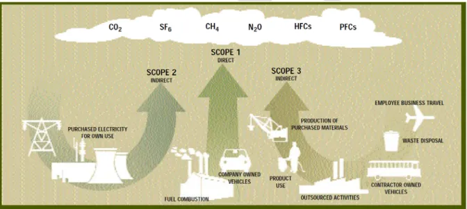
Figure 1: Different scopes of emissions accounting as described by the Greenhouse Gas
Protocol (2008). ... 6
Figure 2: The intended role of Klimakost in management and improvement of environmental impacts for companies and municipalities. ... 8
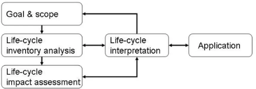
Figure 3: Outline of the stages and iterative approach of life cycle assessment (Adapted from ISO (2006a)) ... 10
Figure 4: Sensitivity analysis of different electricity mixes, Tromsø 2007 ... 18
Figure 5: Consumption based inventory for Norway ... 22
Figure 6: Consumption based inventory for Norway excluding exports ... 23
Figure 7: Impacts from household demand, allocated to consumption categories ... 24
Figure 8: Impacts from household demand, allocated to producing sectors ... 25
Figure 9: Municipal CF (map by Statens kartverk) ... 29
Figure 10: Relating municipal CF to population size and available funds ... 29
Figure 11: Carbon Footprint of different activities/purchases, Lier 2007 ... 30
Figure 12: Carbon Footprint of different areas of responsibility, Lier 2007 ... 31
Figure 13: CF of primary and secondary schools in Tromsø ... 33
MiSA AS, 07.10.2009 Page 5
Introduction
Klimakost1 is a model for calculating life cycle (direct and indirect) emissions for companies, organizations and municipalities in a cost-effective, yet still methodologically concise, manner. The tool is directed towards municipalities and businesses who want to analyze the amount of
direct and indirect emissions from their consumption of goods and services. This type of
perspective is normally referred to as life cycle assessment (LCA), since it aims at tracing all emissions occurring from consumption, all the way back to extraction of raw materials and fuels. The tool has been developed by MiSA AS2, a start-up consultancy in Trondheim, Norway. The founders of MiSA all share a background from the Norwegian university of Science and
Technology, more specifically the Industrial Ecology Program3. This program is well recognized internationally for its development and application of LCA and input-output based methods, and numerous publications in international peer-reviewed journals strengthen its position on a national and international level.
Klimakost is specifically targeted and streamlined towards municipalities and green procurement in the public sector. This is a consequence of the evolutionary process of the tool, and does not exclude use within other segments, but there is still some work needed in streamlining the application in businesses. Innovation Norway4 has supported the development of the tool, facilitating a more updated calculation model and web pages.
Growing concern about indirect emissions
Currently almost all emission statistics focus on direct emission from the studied organization, company, nation or industry. There is, however, a shift in trends to include life cycle
considerations so that supply chain effects are included and accounted for. These effects are often referred to as indirect effects. In this way the consumer is allocated more of the responsibility for emissions, and focus is pointed toward the intricate cause-effect chains between
consumption and production.
Early focus on indirect emissions includes works within input-output analysis and early process based life cycle assessment (Leontief 1970b; Bullard, Clark et al. 1975; Bullard, Penner et al. 1978; Nunn 1980). These studies paved the ground for the later interest in indirect emissions and cause effect chains of energy demand.
During the 1990’s the concept took off and the number of approaches and studies within the field exploded. At present there is a continuous rapid development of the methods used in calculating indirect emissions (see section Methodology on page 8).
International trade studies now demonstrate clearer and clearer the global nature of especially the climate issue, where it is shown how emissions embodied in international trade is significant, and
1 www.klimakost.no 2 www.misa.no 3 www.ntnu.no/oko 4 www.invanor.no
MiSA AS, 07.10.2009 Page 6
that the existence of “pollution havens” may seriously affect initiatives on reducing emissions if these indirect effects are not accounted for. For global data for 2001 see Hertwich and Peters (2009), or visit www.carbonfootprintofnations.com.
For single products the life cycle perspective is included in so-called environmental product declarations of type III (ISO 2000) and other initiatives (British Standards 2008). The ISO standard builds upon the more general standards for life cycle assessment (ISO 2006a; ISO 2006b). The latter however, only includes greenhouse gases, excluding numerous other important pollutants.
The last few years there has been an increasing focus on the same perspective for organizations and companies for instance the Greenhouse Gas Protocol (2009), which was used as background for the new standard for organizational carbon accounts ISO14064-1 (ISO 2006c).
Figure 1: Different scopes of emissions accounting as described by the Greenhouse Gas Protocol (2008).
It is our claim that any serious assessment needs to include scope 1,2 and 3 in a consistent manner. Emissions other than greenhouse gases should also be included; this can be done without significant additional effort. If there is a need to avoid double counting, a consistent procedure to distribute burdens should be used (see section Responsibility sharing at page 27). Several other standards have followed, describing various offsetting schemes, and validation of projects (ISO 2006d; ISO 2006e; ISO 2006f).
Klimakost
As mentioned earlier the development of Klimakost started with a focus on municipalities and the production of municipal public services.
MiSA AS, 07.10.2009 Page 7
The municipalities in Norway can get state funding for developing climate action plans. The requirements for this funding, as defined by state organ ENOVA, now also include mention of indirect emissions:
“Planen bør også omfatte tiltak knyttet til redusert klimagassutslipp fra annen aktivitet i kommunen som kommunen kan påvirke. Det kan være direkte utslipp fra transport, avfallsbehandling og landbruk, og
indirekte utslipp fra innkjøp” 5
EN:”The plan should also include actions aimed at reducing other activities the municipality can affect. It can be direct emissions from transportation, waste treatment or agriculture, as well as indirect emissions from procurement.”
Including indirect emissions consistently for an entire organization is something that currently is not offered by any other Norwegian company than MiSA.
Road ahead
The road ahead for the tool includes further methodological development and improvement, adaptation to new market segments, and last, but not least, the acceptance and approval by authorities that tools exist for calculating scope 3 emissions and that these should be used. Klimakost has received some media attention domestically6 and is also included in Statistics Norway survey of ongoing initiatives for improving municipal statistics (Hoem 2009).
We will also seek to internationalize the tool. Currently there are ongoing initiatives together with partners in Denmark and Sweden.
Intented use in the process of environmental management
Klimakost has an intended use in the mitigation strategy of an organization or company. This is indicated in Figure 2.
It is extremely important to base actions on trustworthy facts, so that resources are not spent on less important parts of the system. To some degree there is a tendency of that today, sine a major part of emissions are overlooked when not employing a full life cycle perspective (i.e. full
implementation of scope 3 in the greenhouse gas protocol). By employing the top-down procedure the figure indicates, such poor prioritizations are minimized.
5http://naring.enova.no/sitepageview.aspx?sitePageID=1301
MiSA AS, 07.10.2009 Page 8
Figure 2: The intended role of Klimakost in management and improvement of environmental impacts for companies and municipalities.
Limitations of Klimakost
Klimakost is very well suited to make first time estimates of emissions on an aggregate level (e.g. identify food purchases as an important contributor to emissions). However, it is not well suited to make detailed prioritizations, such as choosing whether to buy corn or wheat and analyze the effect of this. More detailed studies are needed for such in-depth analyses. This can easily be integrated by hybridizing the model with LCA-data as more focus on certain commodities is required.
Methodology
Klimakost is based on state-of-the-art developments within the field of environmental systems analysis. It is therefore necessary with an understanding of the toolbox presently available within the field. All the methods presented here may be used both to analyze single products and to analyze organizations as a whole, although for all applications special attention must be given to functional differences and the goal and scope of the assessment, to ensure consistency.
Lifecycle assessment
Life-cycle assessment (LCA) is the assessment of environmental impact through the life-cycle of product systems. Cornerstone to the life-cycle approach is the understanding that environmental impacts are not restricted to localities or single processes, but rather are consequences of the
life-MiSA AS, 07.10.2009 Page 9
cycle design of products and services. The product life-cycle covers all processes from extraction of raw material, via production, use, and final treatment or reuse (Wenzel, Hauschild et al. 1997; Guinée 2001; Baumann and Tillman 2004; ISO 2006a). The combination of a quantitative approach and a holistic perspective leads to trade-offs being clearly stated in LCA. It is a systems tool well-suited for environment decision making.
Referred to by many names through its development (Baumann and Tillman 2004), LCA has in the last four decades evolved from the idea of cumulative resource requirements into a scientific field that includes emission inventory methods (Heijungs and Suh 2002) and environmental cause-consequence modeling (Udo de Haes, Finnveden et al. 2002). Many of the first applications, including the first Norwegian use of the life-cycle concept (Nunn 1980), were related to beverage packaging, although early reviews show a large span in the products that were assessed with life-cycle approaches (Nord 1992).
The problem of including all significant processes in life-cycle inventories is a well known in LCA (Norris 2002). Hybrid approaches have been proposed as a method to identify the largest contributing paths and to ensure that all processes are included within the system boundaries (Suh 2004; Suh, Lenzen et al. 2004). Hybrid approaches link process information collected in physical life-cycle inventories with monetary flows in economic models. The combination of LCA and input-output models has shown value as a complementary tool to traditional inventory methods in LCA (Heijungs and Suh 2002; Strømman 2005; Strømman, Solli et al. 2006).
Standardization of LCA methodology has been achieved step by step. The SETAC working groups (e.g., Consoli, Allen et al. 1993; Barnthouse, Fava et al. 1997; Udo de Haes, Finnveden et al. 2002) and other institutions have been vital in this process (e.g., Nord 1992; Nord 1995). The development of international standards has been an important driver for defining the methods of LCA. The first set of standards were published by the International Organization for
Standardization in 1997 (ISO 1997), with a revised version complete in 2006 (ISO 2006a). For a more thorough description of the historical development of LCA, see Ayres (1995) and
Baumann and Tillman (2004).
General framework
The standardized framework for LCA states four consecutive stages, as illustrated in Figure 3 (ISO 2006a). The stages are described in some detail here, but the reader is referred to guidelines and textbooks for a thorough introduction (e.g., Wenzel, Hauschild et al. 1997; Hauschild and Wenzel 1998; Guinée 2001; Heijungs and Suh 2002; Baumann and Tillman 2004; ISO 2006a). Goal and scope
The first stage of LCA consists of defining the aim and boundaries for the assessment, and the choice of methods for inventory and impact assessment.
The goal and scope stage includes defining the functional unit (FU). The functional unit is a quantitative measure of the functional requirement(s) that the product or service is designed to
MiSA AS, 07.10.2009 Page 10
fulfill. It is the basis for comparison in LCA, used to evaluate the relative performance of alternative product systems.
Figure 3: Outline of the stages and iterative approach of life cycle assessment (Adapted from ISO (2006a))
Examples of FUs are 15 years of person transport for transportation systems, 100m2·years for paints
and other surface protectors, and 1 GJ at consumer for energy supply and distribution systems. Life-cycle assessment may be applied for various purposes, such as product benchmarking, product declaration, process development and policy support. Study designs set important limitations on the applicability of the study to provide answers. An important issue in this respect is the functional unit. Other issues include the level of inventory completeness, temporal and spatial considerations, and impact and inventory assessment approaches.
Limitations in scope may be caused by resource constraints. Spatial and temporal limitations may be applied to suit policy perspectives. Similarly, a study may be undertaken to investigate a few issues of concern, such as energy efficiency rates or CO2-equivalents, or it may aim at a broad impact assessment. While limitation of the scope is a necessary step towards completing any study, it is vital that the principle of reproducibility is maintained; i.e., that the eventual limitations do not exclude information that may alter the conclusions.
Life-cycle inventory analysis (LCI)
The second stage consists of establishing an inventory that describes the environmental interventions that arise from the product system. Environmental interventions are inputs of resources from the environment to the product system (i.e., energy and material resources), and outputs to the environmental of adverse effect that the product system produces (i.e., emissions). The inventory is balanced to the functional unit.
Life-cycle impact assessment (LCIA)
Once the inventory of environmental interventions is established, the interventions are translated to environmental impact indicators in the third stage of LCA.
The ultimate purpose of LCA is to provide indication of environmental impact potential. Quantitative scores are achieved by application of characterization factors that describe the
MiSA AS, 07.10.2009 Page 11
relative potential of each intervention to adversely affect safeguard objects through defined impact mechanisms. An example is CO2-equivalents which are used to aggregate the global warming potential of various emissions to air. Each substance is characterized by its potential relative to the global warming potential of CO2.
The life-cycle impact assessment stage is divided into three consecutive steps. First,
environmental interventions are separated according to their cause-and-effect chains, termed impact chains or impact categories in LCA. Interventions may be input-related; i.e., energy and material extracted from the environment, or they may be output-related; i.e., emissions made to the environment. Second, impact scores are aggregated for each impact category by multiplying inventory mass flows with their respective characterization factors and summarizing for each of the impact chains. The last step of life-cycle impact assessment is the weighting of impact scores relative to each other. Weighting requires relative comparison of different environmental issues; such as comparison of acidifying air-emissions with consumption of material resources. An inherently subjective process, and a voluntary step in life-cycle impact assessment, weighting is not often applied in the scientific literature.
Weighting methods and the selection of impact categories to be considered in an LCA depend on the stakeholders to the study. Identification of stakeholder attributes, and the matching of these with the results produced by the study, is vital to ensure the relevance of any LCA. Life-cycle interpretation
The final stage of LCA is the interpretation of results. Vital in the interpretation stage is the consideration of uncertainty. Other aspects include the effect and validity of the selected impact assessment methods to fulfill the stated purpose of the study, and the potential bias introduced by inventory sources and approach. The re-visitation of methodological choices validates the outcome of LCA and increases the relevance of LCA for decision support.
Environmentally extended input-output analysis
Input-output analysis (IOA) was initially developed by Leontief (1936) as a method to study the interrelations between the sectors in an economy. In the beginning of the seventies he
formulated a framework to extend the analysis with environmental information (Leontief 1970a). The basic idea is to utilize the information contained in national economic statistics, in
combination with data on emissions from the various sectors in the economy, to calculate all the (direct and indirect) emissions occurring from an arbitrary final demand placed upon the system. The economic consequences of spending 1 NOK on, say, gasoline, may be calculated and traced through all the interconnected sectors of the economy in an infinite (but converging) series of demands between the sectors. Once the economic outputs required to support the production of this 1 NOK purchase of gasoline have been calculated, the resulting vector of economic activity in each sector may then be multiplied with emissions intensities for each sector to give the total (life cycle) amount of emissions occurring in the production of 1 NOK worth of gasoline.
MiSA AS, 07.10.2009 Page 12
When the emissions are calculated, the procedure that follows may be equal to that of LCA. The approach has been developed significantly developed since Leontief, both for standalone use (Suh and Huppes 2002), multiregional analyses (Peters and Hertwich 2006a; Peters and Hertwich 2008) and structural studies (Peters and Hertwich 2006b; Guan, Hubacek et al. 2008; Guan, Peters et al. 2009).
The structure and compilation of input-output tables for an economy is described in detail in United Nations (1999).
Hybrid life cycle assessment
While process based LCA7 is relatively specific in the type of data used, it has been criticized for leaving out significant portions of the emissions that occur in the system (Lenzen 2001; Norris 2002; Strømman, Solli et al. 2006). This is referred to as cut-off and is particularly true for far upstream processes and service based activities.
On the other hand input-output analysis is good for including emissions from all types of activities without any cut-offs, since it is based on an aggregated model of all existing sectors of the economy. However, it lacks the detail provided by LCA, so that it may be good for
estimating e.g. total emissions from household food consumption, but is not able to distinguish between bread and bananas.
Several authors describe the use of LCA and IOA in a hybrid approach, trying to utilize the benefits of both approaches, both obtaining the completeness associated with input-output analysis, as well as the specificity offered by process based LCA.. Various variants of these approaches are described by several authors (Treloar 1997; Nakamura and Kondo 2002; Suh, Lenzen et al. 2004; Suh and Huppes 2005; Strømman and Solli 2008) and applied to different case studies (Marheineke, Friedrich et al. 1999; Treloar, Love et al. 2000; Lenzen 2002; Solli, Stromman et al. 2006; Strømman, Solli et al. 2006; Michelsen, Solli et al. 2008; Larsen and Hertwich 2009).
Computational structure
The computational structure of life cycle assessment, input-output analysis and hybrid LCA is more or less identical. The idea is to calculate emissions occurring as interconnected processes are instigated by a final demand. Several authors give detailed descriptions on the computational structure of LCA (Heijungs and Suh 2002; Peters 2007) . We will give a short description of the computational framework in the following. Beware that notation may differ from other sources as there is no general agreed-upon nomenclature that apply to all methods.
We start by defining our system of production processes, economic sectors, or both (in hybrid analyses) as a matrix Z, containing the flows of energy, materials, money etc. between the different entities (from now on referred to as “nodes”).
7 The standard/”old fashion” LCA is often described as ”process based LCA” to distinguish it from approaches
MiSA AS, 07.10.2009 Page 13
,
Each element zij of the matrix denotes the flow of the product from node i into the production of output from node i. In addition we have information on the total output from the system, x. If the total output from each node is described by the vector x, a normalized system may be constructed by dividing each column in Z by the corresponding total outputs. The result is a matrix A containing the “cookbook recipe” to produce one unit output from node each node in the system.
Say we want to calculate the total output from each node due to some final demand by an end consumer, for instance a household. The final demand from the various nodes can then be described by the vector y.
Setting up a balance we know that the total output of the nodes subtracted the amounts consumed by the nodes themselves, should equal the final demand y.
The total output x from each node needed to fulfill the demand of the household, in addition to all the intermediate demand from other nodes, can then be calculated by
The Leontief inverse, L, is a matrix describing multipliers for all nodes in the system, so that a column j in L gives the total direct and indirect outputs in all other nodes in order to deliver a unit final demand from j.
Similarly emissions can be treated the same way where the matrix S is total emissions and where an element skj contains the emissions of substance k from node j.
Normalization by dividing of total node output gives a matrix F of emission intensities per unit output from each node.
MiSA AS, 07.10.2009 Page 14
The total emissions e occurring due to an arbitrary final demand from the nodes can now be calculated by
Introducing characterization factors according to the description in section Life-cycle impact
assessment (LCIA) at page 10 gives the opportunity to translate the emissions data into more
understandable environmental impact potentials d. The characterization factors are contained in the matrix C, where an element clk describes the contribution of emission type k to impact category l. the calculation of d then becomes
This is as far as we go in this presentation of computations in life cycle assessment, but the well defined structure of the system enables easy calculation of the contribution of final demands, nodes and/or emissions to the different impacts. This is plain linear algebra and may easily be performed in any mathematical software or in specialized LCA software, such as Simapro8. Further breakdowns and analyses are also possible through structural path analysis, monte-carlo simulations and linear programming techniques. These require more advanced modeling and will not described here.
The background model
Although life cycle assessment is often targeted towards analyzing product or functions, the very same techniques may just as well be used to analyze the impact of entire organizations or
businesses. Klimakost utilized both process-LCA techniques in combination with IOA for its calculations. In addition there are a number of adaptations done for each of the market segments where we utilize the model; municipalities, businesses and households.
A main requirement for Klimakost is an input-output model of the economy which is in the background of the studied entity. We have constructed a model for Norway following the procedure described in section Computational structure at page 12, using national accounts data for Norway from 2005 (Statistics Norway 2009b), and emissions data for the same year (Statistics Norway 2009a).
Capital
The consumption of fixed capital is internalized in the model by assuming this to follow the average structure of the fixed capital formation in the given year. The practical meaning of this is that we allocate the depreciation of fixed capital in 2005 to the production that year, and the difference between fixed capital formation and depreciation is treated as a final demand and may be allocated to the production of tomorrow. This way of internalizing capital is somewhere
MiSA AS, 07.10.2009 Page 15
inbetween the flow-matrix method and the augmentation method described in Lenzen and Treolar (2005)
There is an error introduced by the assumption that the consumption of capital is only
subtracted from the fixed capital formation domestically9. This only affects studies involving the capital formation directly, such as in Figure 5, where the final demand category net capital build-up
is probably overestimated due to a higher share of imports that what is realistic. Imports
Ideally a true multiregional input-output model10 (Peters and Hertwich 2006a; Peters and
Hertwich 2008; Hertwich and Peters 2009) should be used in combination with trade statistics in order to estimate the economic activity and emissions occurring abroad in order to supply domestic demand. These models are hard to come by, and usually suffer from issues regarding lack of data and recency.
We have chosen, so far, to treat imports as if they were produced with domestic technology, except for the electricity generation used to produce imports, where we make changes to the emission factors for the electricity generation sector using data adapted from Dones et al. (2007). Future versions of Klimakost will seek to include true multiregional models when these become available.
UPDATE August 2009: Klimakost is now available with Germany as import country. The number of pollutants is, however, fewer than in the previous model.
Hybridization
More in the detailed adaptations sections.
Included emissions and impact categories
The following pollutants are currently available in Klimakost: CO2 CH4 N2O CO HFCs PFCs SF6 NOx SOx NH3
9 There are a few practical reasons for this. It may change in future versions of Klimakost.
MiSA AS, 07.10.2009 Page 16
NMVOC
PM10
We are currently working on including more types of emissions, but perhaps more important, primary energy use, in the model.
For the characterization of the emission, we use factors from the well-recognized method CML 2 Baseline 2000 v.2.04 (CML 2004) to calculate impact potentials within global warming
(expressed as CO2-equivalents), acidification (expressed as SO2-equivalents), human toxicity (expressed as 1,4-di-chloro-benzene-equivalents), photochemical oxidation (smog) (expressed as C2-H2-equivalents). In addition we report particulate emissions (PM10) as a separate category. Preparations for use
The model is in basic prices, which means that for any use with data in purchaser prices, we need to know or estimate the trade and transport margins, as well as the taxes. In addition we must perform inflation adjustments to the base year of the input output model. These steps are vital
in order to produce a model that can be used in Klimakost assessments. The price adjustments are all performed one an industry specific level, using appropriate data from Statistics Norway. The procedure involves a certain degree of subjective judgment and craftsmanship and the details are not explained here.
Klimakost
The computational structure in Klimakost follows the approach described in section
Computational structure at page 12. There are however, some additional modification related to
the coupling of the hybrid LCA model and the data from the municipalities or businesses. Municipalities
One key feature of the municipalities is their common reporting format KOSTRA11. This ensures consistent reporting from the municipalities to the central government and statistics office at a certain level. This is what initially started the work with Klimakost, the fact that all this information in standardized form is available for use, if there is an appropriate model to connect it to.
The municipal accounting system uses a set of pre-defined 3-digit commodity categories defined in KOSTRA. In addition, most municipalities define sub-categories to these on a 3,4 or 5-digit level. They also report according to function (to be interpreted as municipal departments/areas of responsibility) in the 3-digit standard form defined by KOSTRA, but may have internal categorizations in an even more detailed level (e.g single schools).
This enables two types of analyses based on municipal accounts; one using as basis the standardized 3-digit commodity categories, as well as the function categories. This analysis is
MiSA AS, 07.10.2009 Page 17
extremely cost-effective to perform, as virtually no manual labor is needed once the model has been made. Interpretation, quality check and reporting of results, however, still require input of expert labor.
A more comprehensive and accurate approach is to use the municipalities internal
categorizations on both commodities and departments to produce results. This is a semi-tailor-made approach, as the categories vary across municipalities. More labor is needed to use this data and connect it to the background model, but the results are also more accurate and may be more policy relevant in deciding e.g. commodities that deserve a stronger focus in procurement or use. Connecting the municipal account data with the background model consists of several steps. The first is to create a correspondence matrix H between municipal commodities and the economic sectors in the background model. As described earlier this can be done on the standardized 3-digit level or on the more detailed internal level. The allocation of 3-3-digit commodities to
economic sectors can also be further refined by using more detailed data from the study of other municipalities as the basis for the correspondence matrix H. The rows of H are the economic sectors in the input-output model, and the columns the KOSTRA-classification used. All elements in H range from 0 to 1. The column sum of H must be equal to 1.
Second the prices must be adjusted to the correct base-year and basic prices. The latter involves correcting for taxes in addition to allocating a certain share of all purchases to trade and
transport margins. Both these adjustments are performed on a commodity level using price data from statistics Norway. There is, inevitably, a certain degree of subjective judgment and
craftsmanship involved. The price adjustment data is contained in a vector P, and the allocation of trade and transport margins is contained in the matrix TTM. TTM simply allocates a certain share of each price adjusted purchase to trade and transport margins. Following the approach outlined in the chapter “Computational structure”, the total indirect impacts from a final demand y (y can here be the demand of the entire municipality or some sub-department of the
municipality) can then be calculated by
·
The ” ·” indicates element-wise multiplication as opposed to matrix multiplication.
In addition we have to add the direct impacts (combustion of heating oil, transportation fuels and so on) occurring in the municipality to obtain the total footprint from y.
Some special adjustments are made with respect to the production of electricity and use of liquid fuels. These items are fairly easy to obtain physical data for, and contribute significantly to the emissions from the municipalities. The model is hence hybridized with process based data on these items. In addition specific commodities identified in initial analyses can be further investigated by hybridizing the model with process based LCA data.
MiSA AS, 07.10.2009 Page 18
The model is also constructed so that the electricity mix used can be changed on three levels, depending on assumptions regarding the real (marginal) emissions from electricity consumption. These levels are:
1. Direct electricity use in the municipalities
2. Electricity used to produce products and services in Norway 3. Electricity used to produce products and services abroad The choices of electricity for all levels are:
Norwegian (NO) mix Nordic (N) mix
European (UCTE) mix
UPDATE August 2009. We now have a model with Germany as import nation in addition.
In Figure 4, a sensitivity analysis is performed on different set of choices regarding the production of electricity to the three levels, 1 - 2 - 3, respectively. The sensitivity analysis was applied to the GHG accounting of Tromsø. We see that there is about a factor 2 difference
between the situation where we assume Norwegian electricity mix for all, and when we assume Nordic mix for direct input to the municipality as well as production of goods and services in Norway, and UCTE mix for production of goods and services imported to industry or directly to the municipality.
Emission footprint of the households in a municipality
Several municipalities have approached us asking for footprint calculations for the households within the municipality. These emissions can be calculated with the model (see for instance Figure 7). However, contrary to the municipal accounts, which supply us with large amounts of data on the purchases of that specific municipality, the data basis of household in each
0 5 10 15 20 25 30 35 40 45 50
NO-NO-NO NO-NO-UCTE N-NO-UCTE N-N-UCTE
Carbon Footprint of Tromsø [1000 tonnes CO2 equivalents]
Direct GHG emissions Indirect GHG, Tromsø Purchase of electricity by municipality Indirect GHG, Norway Indirect GHG, Abroad
MiSA AS, 07.10.2009 Page 19
municipality, is much less specific. On a national level, we have good data for households
through the national accounts and the survey of consumer expenditure (SCE). The SCE only has 2000 respondents, far from sufficient to supply representative data for individual municipalities. The breakdown of household footprints to municipality level has thus been performed by scaling with the income level of the inhabitants in each municipality. This means we assume the structure
of consumption to be the same everywhere, and just scale the total volume of consumption. In future analyses we may find ways of improving this approach.
Businesses
Klimakost for businesses is still in development. We see two potential paths for the tool:
A generic tool with sectoral adaptations. This will be a simplified approach for small businesses and may be presented with a web-based interface.
Tailor-made solutions for large companies, integrating the footprint calculations into their environmental management system
Since businesses have no final demand, the allocation of all emissions to final demand (as done in the previous figures) renders businesses without any responsibility for emissions. On the other hand, allocating all emissions from a company’s inputs to that specific company may result in double counting of emissions if the same perspective is used in other companies in their supply chain (or their downstream customers). Some companies still want to do this assessment. However, there is a mathematically consistent way of allocating the emissions between producer and consumer in each sted in the supply chain, going back an infinite amount of steps.
Any split (from 0 to 1) of responsibility between producer and consumer can be made. We currently work on implementing this responsibility sharing feature in Klimakost. The household calculator
For the household calculator on our web pages, we have used a slightly different model, including more multiregionality at the expense of recency. It is based on input-output data contained in the GTAP model (GTAP 2006). It should be noted that this calculator only
includes CO2-emissions and no other greenhouse gases, in contrast to the model that Klimakost is based upon. The first version of this was originally developed at the Industrial Ecology
Program in collaboration with Glen Peters, and an earlier version is found on the web pages of the national broadcaster NRK (NRK 2007).
Uncertainties
Klimakost is without a doubt the most precise and cost-effective tool of its kind in Norway. To our knowledge no other systematic and methodologically consistent tools exist at present. There are, however, many inconsistent, incomplete and inaccurate tools and providers in the market.
MiSA AS, 07.10.2009 Page 20
This does not mean that Klimakost is perfect. There are, inevitably, several sources of uncertainty connected to use of Klimakost for municipalities:
Uncertainty in the background model
Uncertainty in the price adjustments (from purchaser prices to basic prices, and from different base years)
Uncertainty in the assumption of equal prices across municipalities Uncertainty connected to varying practices in municipal book-keeping
Uncertainties caused by the aggregated nature of the background model, the municipal account categories (“arter”) and the (mis)match between economic sectoral definitions and municipal purchases.
Different
responsibility
perspectives
and
some
results
for
the
Norwegian
economy
Based on the input-output model we have made calculations for Norway for 2005. This example illustrates various point regarding different calculation perspectives and how this affects emission inventories. Issues regarding different calculation perspectives have been defined and explored by several authors in the past (Bastianoni, Pulselli et al. 2004; Lenzen, Murray et al. 2007; Peters 2008), giving a substantial body of literature to build a model upon.
For reasons of simplicity greenhouse gas emission, expressed as CO2-equivalents, is used in most of
the discussions, if not otherwise specified.
For the production of these results, we have assumed average Norwegian electricity used domestically and European mix (UCTE) for imports. However, the electricity mix can be changed and the effect of this easily investigated within the model.
Production perspectives
Both of the perspectives below belong to a “production perspective”, where responsibility for emissions is with the actual emitting industries or the emitting country.
Geographic/Kyoto perspective
The emissions from geographic Norway, or more precisely the emissions as defined in the Kyoto agreement were 54 million tons in 2005 (Statistics Norway 2008).
National account perspective
In contrast the 2005 emissions stemming from all Norwegian economic activity were about 65 million tons (Statistics Norway 2009a). This increase is mainly due to the inclusion of emissions intensive activities not occurring on Norwegian soil, such as shipping and international air travel.
MiSA AS, 07.10.2009 Page 21
Consumption perspective
Norwegian economic activity, and hence emissions thereof, is driven by the following final demands
Households
Governmental demand Capital demand
Changes in stock (CIS) Exports
In addition we have import demands from final consumption categories (above) and through intermediate demand from the industries.
There are also emissions occurring directly in the households from activities such as combustion of wood or oil for heating and gasoline/diesel for transportation.
As soon becomes clear, a large portion of the emissions occurring in Norway, are caused by export demand. Vice versa, Norwegian demands instigate activity and emissions in countries we import from.
Allocated to consumption categories
The consumption based impact potentials of emissions from Norwegian final demand are shown in Figure 5. It is evident that export demand is a major driver of emissions. Note that all the final demands instigate imports, so that even the export demand causes emissions in countries we import from.
Assuming the emissions caused by export demand is the responsibility of the countries who import this, we are left with the domestic final demands. The environmental footprint of these is shown in Figure 6. Figure 6 is the same as Figure 5 with export taken out. We see that for global warming (carbon footprint) it is the household demand that causes the largest emissions. The households are responsible for the emissions of about 36 million tonnes (mt) CO2-eq. 29.7 mt is indirect emissions from the production of goods and services instigated by household demand, 5 million tonnes are from direct emissions from transportation, 1.1 mt from household heating (oil furnaces) and 0.123 mt from other sources. Governmental demand, changes in stock and net capital accumulation causes the remainder of emissions.
MiSA AS, 07.10.2009 Page 22
Figure 5: Consumption based inventory for Norway
In other types of environmental impacts this distribution is different. This is most pronounced in the smog formation category, as well as the category for particle emissions. For particles, the large contribution from household heating is due to heating by wood stoves. For smog formation it is the transport emissions and wood stove emission that cause these categories to have a high share of the total impact.
If we look more closely at the household demand (Figure 7) we can distribute the footprints on different consumption categories. The categories have been sorted by relative importance in the global warming category. We see that the direct emissions from transportation is the most important category for global warming, followed by the use of hotels and restaurants abroad, food, real estate services, transport services (not own vehicle, but purchased transport) and imported food. This does not mean that hotels and restaurants abroad are particularly dirty
29 711 181 868 242 865 15 392 11 161 7 060 35 973 58 177 4 152 2 764 4 945 8 704 36 440 9 390 778 1 101 1 592 37 385 5 309 35 699 123 ‐ 5 433 886 1 027 3 638 18 042 27 681 1 657 1 283 4 977 35 678 45 819 2 212 2 167 61 637 350 837 618 417 38 042 23 333 0 % 10 % 20 % 30 % 40 % 50 % 60 % 70 % 80 % 90 % 100 %
kt CO2‐eq. t SO2‐eq. t 1,4 DCB‐eq. t C2H2‐eq. t PM10
Global warming Acidification Human toxicity Smog Particulates
Households Government Households, direct, transport
Households, direct, heating Households, direct, other Changes in stock
MiSA AS, 07.10.2009 Page 23
industries; the importance is purely a result of a large volume of consumption, and the fact that
upstream activities to this sector have much larger emissions, especially electricity production.
Figure 6: Consumption based inventory for Norway excluding exports
The other types of impact more or less follow the same ranking as the carbon footprint, except for some small differences. Note that the direct emissions from household heating totally dominate the particle emission footprint, which also affects the smog formation and human toxicity categories.
Generally we see that the footprints are distributed across a very wide range of goods and services. For all impacts there is a quite large fraction contained in the “remaining” category of purchased goods and services; this is the sum of about 100 other consumption categories.
29 711 181 868 242 865 15 392 11 161 7 060 35 973 58 177 4 152 2 764 4 945 8 704 36 440 9 390 778 1 101 1 592 37 385 5 309 35 699 123 ‐ 5 433 886 1 027 3 638 18 042 27 681 1 657 1 283 4 977 35 678 45 819 2 212 2 167 0 % 10 % 20 % 30 % 40 % 50 % 60 % 70 % 80 % 90 % 100 %
kt CO2‐eq. t SO2‐eq. t 1,4 DCB‐eq. t C2H2‐eq. t PM10
Global warming Acidification Human toxicity Smog Particulates
Households Government Households, direct, transport
Households, direct, heating Households, direct, other Changes in stock Net capital build‐up
MiSA AS, 07.10.2009 Page 24
Figure 7: Impacts from household demand, allocated to consumption categories
Household emissions allocated to producing sectors
We can allocate emissions to either final consumption categories or producing sectors. In the previous figures we allocated the emissions to consumption categories. The emissions do not occur
there, but in all upstream processes required to deliver this final demand. We can calculate where
these emissions occur by simple mathematical manipulation.
Figure 8 shows the emissions caused by household demand, allocated to the sectors where they
actually occur. We now see that electricity production in importing countries is the largest cause of
emissions, since this is used as an input in the production of goods and services that are consumed by Norwegian households directly or indirectly through import to industry.
0,0 % 10,0 % 20,0 % 30,0 % 40,0 % 50,0 % 60,0 % 70,0 % 80,0 % HH Transport (Import)_Hotels and restaurants Manufacture of food products and beverages Real estate activities Land transport; transport via pipelines (Import)_Manufacture of food products and … Agriculture, hunting and related service … Wholesale trade and commission trade, … (Import)_Agriculture, hunting and related … Manufacture of chemicals and chemical … HH heat (Import)_Manufacture of chemicals and … Hotels and restaurants Retail trade, except of motor vehicles and … Supporting and auxiliary transport activities; … (Import)_Manufacture of motor vehicles, … Water transport Air transport Sale, maintenance and repair of motor … Manufacture of motor vehicles, trailers and … Remaining
Global warming kt CO2‐eq. Acidification t SO2‐eq. Human toxicity t 1,4 DCB‐eq.
MiSA AS, 07.10.2009 Page 25
Figure 8: Impacts from household demand, allocated to producing sectors
Further breakdown of results
Various types of breakdown of results are possible using Klimakost. For instance we can show the contribution of different stressors to the included types of environmental impact.
In addition we can perform a so-called structural path analysis of the system to better understand how impacts are instigated through final household demand, creating demands throughout the economy, and finally leading to emissions in some specific economic sector.
0 % 10 % 20 % 30 % 40 % 50 % 60 % 70 % 80 % (Import)_Electricity, gas, steam and hot water … HH Transport Agriculture, hunting and related service … (Import)_Agriculture, hunting and related … Land transport; transport via pipelines (Import)_Manufacture of chemicals and … Manufacture of chemicals and chemical … HH heat Water transport Sewage and refuse disposal, sanitation and … Air transport (Import)_Manufacture of basic metals Manufacture of other non ‐ metallic mineral … Extraction of crude petroleum and natural … (Import)_Extraction of crude petroleum and … (Import)_Manufacture of other non ‐ metallic … Fishing, operating of fish hatcheries and fish … Construction (Import)_Land transport; transport via pipelines Manufacture of basic metals Remaining
Global warming kt CO2‐eq. Acidification t SO2‐eq. Human toxicity t 1,4 DCB‐eq.
MiSA AS, 07.10.2009 Page 26
Such breakdowns of results are vital in refining and quality checking the results of an analysis. It also helps identifying areas of the system that deserve more attention with respect to both action and further analysis.
Structural path analysis – unraveling the causeeffect chains of demand and
production
The use of structural path analysis (SPA) to understand and link the consumption (demand) side with the production side is sometimes useful to investigate the cause-effect chain of how
emissions occur in the studied system. This is also useful for quality control. An example of this for global warming potential from the household demand in Norway is shown in Table 1. We have included the 30 top ranking paths, totaling approx. 66% of the total global warming impact. Note that the total number of paths is infinite.
The table should be read as follows: the actual emissions occur in the sector indicated in the last column with text in it. This means that for the top ranking path, emissions occur directly in household combustion of fuels for transportation. For the second ranking path it is the use of restaurants and hotels abroad that instigates activity in electricity production abroad. This in turn lead to emissions in the electricity production sector, amounting to 4,4% of the total national emissions.
Table 1: Ranked structural paths for global warming
Contribution Path
16,6 % Household direct emissions,
transport
4,4 % (Import)_Hotels and restaurants (Import)_Electricity, gas, steam and
hot water supply
4,0 % Land transport; transport via
pipelines
3,7 % Household direct emissions,
heating
3,3 % Agriculture, hunting and related
service activities
2,4 % (Import)_Agriculture, hunting and
related service activities
2,4 % Manufacture of food products
and beverages
Agriculture, hunting and related
service activities
2,2 % Manufacture of chemicals and
chemical products
1,8 % (Import)_Manufacture of
chemicals and chemical products
1,7 % Water transport
1,5 % (Import)_Electricity, gas, steam
and hot water supply
1,2 % (Import)_Manufacture of motor
vehicles, trailers and semi‐trailers
(Import)_Electricity, gas, steam and
hot water supply
1,2 % Air transport
1,1 % Sewage and refuse disposal,
sanitation and similar activities
1,0 % (Import)_Manufacture of food
products and beverages
(Import)_Agriculture, hunting and
MiSA AS, 07.10.2009 Page 27
0,9 % (Import)_Manufacture of
chemicals and chemical products
(Import)_Electricity, gas, steam and
hot water supply
0,7 % (Import)_Manufacture of pulp,
paper and paper products
(Import)_Electricity, gas, steam and
hot water supply
0,7 % (Import)_Manufacture of food
products and beverages
(Import)_Electricity, gas, steam and
hot water supply
0,7 % (Import)_Agriculture, hunting and
related service activities
(Import)_Electricity, gas, steam and
hot water supply
0,5 % Electricity, gas, steam and hot
water supply
0,5 % Other service activities
0,5 % Manufacture of food products
and beverages
Manufacture of food products and
beverages
Agriculture, hunting and related service
activities
0,4 % Manufacture of food products
and beverages
0,4 % (Import)_Manufacture of
furniture; manufacturing n.e.c.
(Import)_Electricity, gas, steam and
hot water supply
0,4 % Household direct emissions, other
0,4 % Supporting and auxiliary transport
activities; activities of travel
agencies
Land transport; transport via
pipelines
0,4 % (Import)_Manufacture of wearing
apparel; dressing and dyeing of
fur
(Import)_Electricity, gas, steam and
hot water supply
0,4 % Manufacture of food products
and beverages
Fishing, operating of fish hatcheries
and fish farms; service activities
incidental to fishing
0,4 % (Import)_Hotels and restaurants (Import)_Manufacture of food
products and beverages
(Import)_Agriculture, hunting and
related service activities
0,4 % Manufacture of motor vehicles,
trailers and semi‐trailers
(Import)_Manufacture of basic metals (Import)_Electricity, gas, steam and hot
water supply
Responsibility sharing
In order to have a consistent allocation of emissions in the value chain and avoid double counting, one can introduce responsibility sharing between the producers and consumers. This can be done mathematically for any chosen split of responsibility in the entire supply network
(Gallego and Lenzen 2005; Lenzen, Murray et al. 2007).
This feature will be included in future versions of Klimakost but is not a prioritized task at the moment.
Extended producer responsibility
Yet another perspective is that of extended producer responsibility. This means that the producer of a product to some or full degree is given the responsibility of emissions occurring downstream of their own production. An example could be a car manufacturer that is given responsibility of the downstream emissions from their cars, both in the use phase, and in the end-of-life phase. This will place incentives on them to develop more emissions efficient cars and systems for recycling and waste handling when the cars are scrapped.
The idea behind the concept is to place incentives for improvements where it has most impact, i.e. in the design phase of a product. One response seen from some companies has been to
MiSA AS, 07.10.2009 Page 28
deliver the services of their products, rather that the products themselves. In this way it is easier to control the performance of the product in the use phase and end-of-life phase. Photocopier company Xerox has experimented with this approach (King, Miemczyk et al. 2006).
This type of approach may work well for some types of products or services while for others it makes less sense. This applies to e.g. bulk material production, fuel production and so forth. This type of perspective is not included in Klimakost and at present there are no plans of including it.
MiSA AS, 07.10.2009 Page 29 102 103 104 105 106 0 0.5 1 1.5 2 2.5 3 Population C a rbon F o o tprint [ tonn es C O 2 equiv a lent s p e r c apit a ]
10 most wealty municipalities High available funds Medium available funds Low available funds
Most populated municipalities, unclassified
Some
aggregated
(3
digit)
results
from
an
analysis
of
all
Norwegian
municipalities
The Klimakost model has been used to derive estimates of CFs for all Norwegian municipalities. 3-digit-KOSTRA, the standardized municipal accounting system, was applied. The result, illustrated in Figure 9, show a large variation from less than half a ton to almost 3 ton of CO2 equivalents per capita resulting from the municipal provision of services.
Per capita CFs further enables us to investigate influential parameters. In the case of municipal CF, in particular two parameters are identified as important; the size of the municipality (population and density) and wealth (available funds). This is illustrated in Figure 10.
The results shown have generated a great deal of interest, resulting in several news items and publications12
12 http://www.cicero.uio.no/klima/09/3/klima09-03.pdf
Figure 9: Municipal CF (map by Statens kartverk)
MiSA AS, 07.10.2009 Page 30
0 0,5 1 1,5 2 2,5 3 3,5 4
Medical equipment Purchase from counties Purchase/renting of machinery Medical materials Insurance, security etc. Purchase/renting of means of transportation Advertising, commercials, information Purchase from the government Other payments/allowances Repair and service contracts Office supplies Medications Renting of buildings Travell allowances Post, bank, etc services Purchase from other municipalities Fees, licences Consultancy Materiels for maintenance Teaching materiels Equipment Courses and training Purchase from municipal collaborating projects Other materiels Food Maintenence of buildings Fuel for transportation Purchase from the private sector Cleaning and caretaker services of buildings Energy
Carbon Footprint [1000 ton CO
2 equivalents]
Administration Education Health Buildings Water sup., sewage Culture, sports etc. Other
Some
results
from
Lier
(3
digit
analysis)
To exemplify a 3-digit Klimakost analysis, we provide some results from the GHG accounts of the municipality of Lier, developed by MiSA spring 2009. The results of a 3 digit analysis is limited to a fixed set of 30 activities/purchases shown in Figure 11, and 33 departments (areas of responsibility) as shown in Figure 12.
The fixes 3 digit KOSTRA set is suited as an overall estimate of contributing elements to the CF. Standardized comparison between municipalities and yearly updates are easy to make. However, some weaknesses have been identified, in particular the aggregation of the important “purchase of Energy”, where no information on the energy composition is available at this level of detail. Because of this, applying a 3-digit- analysis often requires additional physical data on the different purchases of energy made by the municipality.
A 3-digit-KOSTRA analysis could be a very good starting point for small and medium sized municipalities, in addition to clusters of collaborating municipalities wanting comparable and
MiSA AS, 07.10.2009 Page 31
0 0,5 1 1,5 2 2,5 3 3,5 4
Other Before- and after- school care Sludge removal Child welfare services Preliminary work for industry Adult education Activities for children and youth Preschool: housing and transport Political administration Production of water Special schools Library Child welfare actions Prevention measures; health etc. Buildings for municipal disposal Prevention measures; social work Other cultural activities Fire protection Distibution of water Activation of elderly and physically disabled Administration buildings Sewer system Sewage treatment Preschool Healthcare: treatment and rehabilitation Healthcare: home nursing Administration Healthcare: institution Sports Primary and secondary school Housing in institutions Management and maintenance of infrastructure Education: building and transport of children
Carbon Footprint [1000 ton CO2 equivalents]
Energy Transport Infrastructure Materiel and equipment Purchase from other actors / other standardized GHG accounting. For larger municipalities, with a much higher level in their annual accounts, we recommend doing a full 5-digit KOSTRA analysis.
Some
results
from
Tromsø
(In
depth
5
digit
KOSTRA
analysis)
For more in depth information on the composition of the CF, a 5-digit-KOSTRA analysis is performed. This was applied to the municipality of Tromsø in the development of their GHG account report. In addition to an overall GHG account overview, shown in table 3, the 5 digit KOSTRA offers much more detail in the purchases/activities contributing to the CF of each department. In table 4 this is illustrated for the School department of Tromsø. The 38 most contributing activity/purchases are listed showing the large degree of detail provided in assessing the CF.
MiSA AS, 07.10.2009 Page 32
Table 3: Overall GHG accounts of Tromsø, 2007
Department Energy Transport Infrastructure Materiel Equipment Services Other SUM
Political organizing 0 68 0 84 7 4 56 219 Administration 0 151 17 148 52 9 452 830 Buildings 9 577 210 4 852 39 86 177 2 201 17 141 School 42 1 406 76 1434 443 502 953 4 857 Kindergartens 0 144 33 473 148 2 564 510 3 872 Primary healthcare 27 63 16 171 36 660 432 1 405 Social services 267 199 65 82 53 267 683 1 617 Healthcare services 73 1265 44 1 493 246 457 1 023 4 601 Child welfare 0 311 4 7 6 222 344 894 Culture 23 249 32 170 211 54 716 1 454
Roads and parks 1 028 1 316 5 082 107 31 18 148 7 730
City development 0 63 2 21 16 1 177 279
Fire & rescue 0 173 16 41 86 14 73 400
Water & sewage 536 189 835 30 22 4 277 1 893
Other services 2 46 210 105 117 224 905 1 610
SUM 11 576 5 854 11 282 4 405 1 559 5 177 8 949 48 802
Table 4: Overall GHG accounts of Tromsø, 2007
# Activity / purchase of CO2-eq. # Activity / purchase of CO2-eq.
#1 Conveyance of pupils 763 #21 Materiel for arts and crafts 65
#2 Food 373 #22 Raw materials 61
#3 Purchase of special education 271 #23 Meeting and conferences 60
#4 Renting means of transportation 255 #24 Equipment and toys 56
#5 Books for educational purposes 254 #25 Hosting; Food and drinks 48
#6 Course and training 241 #26 Telephone services 44
#7 Travel expenses 215 #27 Filing required travel expenses 43
#8 Miscellaneous services 212 #28 Electricity 42
#9 Purchase from other municipalities 207 #29 Licenses and fees 38
#10 Equipment 200 #30 Conveyance special education 30
#11 Teaching material 175 #31 Cleaning service 27
#12 Paper for educational purposes 135 #32 Welfare arrangements 20
#13 Computer equipment 134 #33 Books for school libraries 19
#14 Other materials 101 #34 Purchase from private comp. 18
#15 Food for educational purposes 91 #35 Papers and literature 18
#16 Office supplies 88 #36 Advertising 17
#17 Renting of buildings 76 #37 Software 14
#18 Conveyance of injured pupils 76 #38 Allowance 14
#19 Renting of office machinery 70 --- Other (account #39 - #293) 216
MiSA AS, 07.10.2009 Page 33 0 100 200 300 400 500 600 'Sto relv a sk ole' 'Skj elna n sk ole' 'Pre stva nnet sko le' 'Kal dfjo rd s kole ' 'Kva løys letta sko le' 'Tro mst un s kole ' 'Sta kkev ollan skol e' 'Bor gtun sko le' 'Sol nese t sko le' 'Kro ken skol e' 'San dnes sund sko le' 'Rei nen skol e' 'Ham na s kole ' 'Sle ttael va s kole ' 'Som mer lyst sko le' 'Bje rkak er s kole ' 'Kro kelv dale n sk ole' 'Sel nes skol e' 'Grø nnås en s kole ' 'Mor tens nes skol e' 'Lun heim sko le' 'Fag eren g sk ole' 'Gyl lenb org skol e' 'Wor kinnm arka sko le' 'Tro msd alen sko le' C a rbon F ootpri n t [K g C O2 equi v al ents per pupi l] Other
Purchase of services from others
Equipment
Food
Materiels for educational purposes
Conveyance of pupils
In addition, departments and area of responsibilities can be divided further into
sub-departments, e.g. dividing the school department into single school buildings. This is illustrated in figure 13 where the CF of single school buildings in Tromsø are normalized by the number of pupils and ranked according to the CF per pupil.
A part of the delivery to a municipality is a calculator that presents the results in an interactive and clear manner.
See http://www.klimakost.no/content.php?cID=66 for the calculator from Tromsø municipality (note that schools have been investigated in extra detail) and
http://misa.no/inhold/lier_kommune/68/ for the calculator from Lier municipality.