Extended Method for Several Dichotomous Covariates to Estimate the Instantaneous Risk Function of the Aalen Additive Model

Volume 17 | Issue 1 Article 27

12-3-2018

Extended Method for Several Dichotomous

Covariates to Estimate the Instantaneous Risk

Function of the Aalen Additive Model

Luciane Teixeira Passos Giarola

Federal University of São João del Rei, [email protected] Mario Javier Ferrua Vivanco

Federal University of Lavras, [email protected] Marcelo Angelo Cirillo

Federal University of Lavras, [email protected] Fortunato Silva Menezes

Federal University of Lavras, [email protected]

Follow this and additional works at:https://digitalcommons.wayne.edu/jmasm

Part of theApplied Statistics Commons,Social and Behavioral Sciences Commons, and the

Statistical Theory Commons

Recommended Citation

Giarola, Luciane Teixeira Passos; Vivanco, Mario Javier Ferrua; Cirillo, Marcelo Angelo; and Menezes, Fortunato Silva (2018) "Extended Method for Several Dichotomous Covariates to Estimate the Instantaneous Risk Function of the Aalen Additive Model," Journal of Modern Applied Statistical Methods: Vol. 17 : Iss. 1 , Article 27.

DOI: doi: 10.22237/jmasm/1543852660

doi: 10.22237/jmasm/1543852660 | Accepted: December 14, 2017; Published: December 3, 2018. Correspondence: Luciane Teixeira Passos Giarola, [email protected]

Extended Method for Several

Dichotomous Covariates to Estimate the

Instantaneous Risk Function of the Aalen

Additive Model

Luciane Teixeira Passos Giarola

Federal University of São João del-Rei São João del-Rei, Brazil

Marcelo Angelo Cirillo

Federal University of Lavras Lavras, Brazil

Mario Javier Ferrua Vivanco

Federal University of Lavras Lavras, Brazil

Fortunato Silva Menezes

Federal University of Lavras Lavras, Brazil

The instantaneous risk function of Aalen’s model is estimated considering dichotomous covariates, using parametric accumulated risk functions to smooth cumulative risk of Aalen by grouping the individuals into sets named parcels. This methodology can be used for data with dichotomous covariates.

Keywords: Aalen’s model, instantaneous risk function, smooth, parametric

distributions, dichotomous co-variables

Introduction

A key question is: what is the risk of an individual experiencing a certain event? There are a variety of models which allow the risk to be studied and to investigate the set of factors which affect it. The interest lies in the non-parametric model proposed by Aalen (1980; 1989; 1993), which is based on counting process theory (Aalen, 1978). It allows the evaluation of the effect of covariates on the risk of failure along time through the cumulative regression functions. The risk of a specimen experiencing an event is modeled from these regression functions, where each regression function corresponds to the difference between the risks of two groups, representing the additional risk of failure of one group in comparison to the reference group. Therefore, in the process of estimating a regression function, a risk

of failure is estimated, additionally. More details about the Aalen model and its applications can be found in Aalen (1978; 1980; 1989; 1993), Gandy and Jensen (2005), Henderson and Milner (1991), and Pereira (2004).

The Aalen model estimates cumulative risks through estimations of the cumulative regression functions, which do not inform the risk of failure that an individual has at a particular instant of time. However, it is more interesting to estimate the instantaneous risk, because it allows knowing the risk of failure at each instant of time, making it possible to make predictions. For this reason, in the Aalen model, it is necessary to estimate the instantaneous regression functions. This can be done using smoothing methods.

A known smoothing method is kernel smoothing, which proposes an estimate for the regression function based on choice of bandwidth and of kernel function. The bandwidth determines the degree of smoothing to be performed; it is responsible for how rapidly the density function oscillates. If the parameter value is too small, an estimated density will present a lot of oscillation; if it is too large, the estimate will be super smoothed (Lima, 2007). Thus, it is necessary to find a bandwidth that minimizes these problems.

The choice of the kernel function is independent of the bandwidth. The kernel function is, in general, a probability density function. Several kernel functions may be used: Gaussian, Epanechnikov, Uniform, Triangular, among others. Different choices presented in the literature for bandwidth are found in Aydemir and Biller (1997), Fahrmeir and Tutz (1996), and Silverman (1986); and for the kernel function in Aydemir and Biller (1997), Keiding and Andersen (1989), Lima (2007), and Ramlau-Hansen (1983).

Despite the good properties of the kernel estimator, it presents some problems regarding the choice of the bandwidth and the tail problem. Aydemir and Biller (1997) evaluated the use of different choices for the bandwidth and indicated the choice of the kth nearest neighbor as the best smoothing method. They also examined the tail problem, but only in the right tail. Keiding and Andersen (1989) proposed a kernel function to solve the tail problem, but Aydemir and Biller, when using this kernel function, obtained regression functions overestimated at the beginning of the observation period compared to the cumulative regression functions.

Lima (2007) compared some methodologies of data-based bandwidth selection considering different approaches of kernel estimation and identified the advantages, disadvantages, and characteristics of each methodology. He concluded that there is not a prominent methodology to estimate densities.

Another way to smooth a non-parametric function is to use parametric models, which are adjusted to the data of this function. In this way, knowing the mathematical expression for the function, it could be mathematically differentiated. Grunkemeier, Jin, Im, Holubkov, Kennard, and Schaff (2006) estimated the instantaneous risk function considering only one additional covariate. They showed it was possible to use a parametric distribution to smooth the non-parametric function of cumulative risk when survival data is available in the presence of a single covariate and, thus, estimate the instantaneous risk function of the Aalen model as a function of this covariate. The question remains: how to estimate the instantaneous risk of failure of the Aalen model for the case in which more than one covariate is presented?

This aim of this study is to estimate the instantaneous risk function of the Aalen model considering, initially, two covariates and, later, generalizing the proposed methodology for several covariates. This is done in order to obtain mathematical expressions for the instantaneous regression functions of the Aalen model from the smoothing by a known parametric distribution and, through them, predict the additional instantaneous risk of one group in relation to another.

Although studies on the additive risk models were developed (e.g., Ma, Kosorok, & Fine, 2006; Lin & Ying, 1994; Martinussen & Scheike, 2009), no estimation method for the instantaneous regression function of the Aalen model, considering several covariates, is as simple as proposed herein and no study presents a mathematical expression for this function that is equally simple.

The Aalen Model

Aalen (1980) proposed a model for survival data that assesses the influence of covariates on the risk of failure over time. This model is non-parametric and does not require initial assumption; it only assumes that the occurrence of the event is independent among the individuals. Several applications of this model have been presented. Mau (1986) investigated the effect of age on the risk of death for patients with lung cancer. Pereira (2004) assessed the risk of early weaning of children up to 18 months old considering some covariates, such as the maternal concept of the ideal breastfeeding time. Grunkemeier et al. (2006) evaluated the risks of bleeding, thromboembolism, endocarditis, and the risks of major paravalvular leak related to the implantation of two types of heart valves. Mansourvar and Martinussen (2017) applied the Aalen model to an observational data set of patients after an acute myocardial infarction event. Başar (2017) also used the Aalen model to analyze kidney transplant data. The Aalen model is described below.

Let r denote the number of covariates in the analysis. The risk function, λi(t),

for the survival time t of the ith individual in the Aalen model is a linear combination of the values of covariates and is given as follows:

( )

0

( ) ( )

( ) ( ) ( )

1 λ_i β Y_i r β_j Y_i Z_ij j t t t t t t = = +



(1)

where Yi(t) is the function indicating whether the ith individual is a member of the

risk set at time t; β0(t) is the baseline risk function, the risk for individuals with zero value in all covariates at time t; Zij(t) is the observed value at time t of the jth

covariate for the ith individual; and βj(t) is the regression function that measures the

effect of the jth covariate at time t on λi(t).

The regression functions are functions of time and their analysis may indicate how the influence of covariates on the failure risk changes over time. This is an advantage of the model.

Let n be the number of individuals observed over a period of time to verify the occurrence of a specific event, which is independent among individuals. The Aalen model for the vector of risks, λi(t), i = 1, 2,…, n, is written as follows:

( )

t =

( ) ( )

t t

λ Z β (2)

where β(t) = (β0(t), β1(t),…, βr(t))ˈ is the vector whose elements are the regression

functions that measure the influence of the respective covariates and Z(t) is the

n× (r + 1) matrix represented in equation (3):

( )

( )

( ) ( )

( ) ( )

( )

( ) ( )

( ) ( )

( )

( ) ( )

( ) ( )

1 1 11 1 1 2 2 21 2 2 1 Y Y Z Y Z Y Y Z Y Z Y Y Z Y Z r r n n n n nr t t t t t t t t t t t t t t t t       =_{ }       Z L L M M O M L (3)

If the event considered has not happened for the ith individual and it is not censored, that is, if it is at risk at a time t, then, the ith _{row of Z(t) is the vector}

Zi(t) = (1 Zi1(t) Zi2(t) … Zir(t)), in which Zij(t) is the value of the jth covariate for

the ith _{individual. On the other hand, if the individual is not at risk at time t, then,} the corresponding row of Z(t) is null.

The Aalen model considers that covariates act additively to the function of risk base and the regression functions are non-parametric functions of time; thus, the cumulative regression functions

( )

( )

0

B_j t =



tβ_j s ds are estimated.

Let t1 < t2 <…< tk <… be the ordered failure times; the estimator for Bj(t)

proposed by Aalen (1980) is given by

( )

( )

ˆB k j k k t t t  =



X I (4)

where X(t) is the generalized inverse of Z(t) (equation (3)), usually defined by

X(t) = [Z(t)ˈZ(t)]–1Z(t)ˈ, and Ik is a vector of zeros except for the individual who

experienced the event at time tk. However, because of the way the matrix Z(t) is

built, the estimator B̂j(t) is only definable as long as Z(t) has full rank, and so, is

invertible. Let τ be the time at which this happens; then the estimation is possible only in the time range [0, τ].

To verify if a covariate has any influence on the survival of individuals, a test can be formulated by the following null hypothesis for the jth covariate:

( )





H : β_{j j} t =0 t, j 1, ,K r

The estimator suggested by Aalen (1989) uses the jth element, Uj , of the vector

given by

( ) ( )

1 K t K t t t t = =



U K X I (5)

with the diagonal matrix K(t) = {diag[(Z(t)ˈZ(t))–1]}–1. These test statistics are possible only in the time range [0, τ]. The test statistic U presents an asymptotic multivariate normal distribution.

Estimation of the Instantaneous Risk Function of the Aalen Model Considering One Dichotomous Covariate

Grunkemeier et al. (2006) developed a study to compare the effect of two treatments which consisted of the implantation of two heart valves: a conventionally used one, and another named Silzone. The authors wished to evaluate the effect of the Silzone valve on the risk of failure compared to the effect

of the conventional valve. Therefore, there was only one risk factor (covariate) in the study: the valve type.

The expression for the cumulative risk of the Aalen model for the ith

individual in the study is

( )

0

( )

1

( ) ( )

Λ_i t =B t +B t Z_i t (6)

where Zi(t) is the value of the valve-type covariate for the ith individual, which

assumes the value 1 for the individuals who have the Silzone valve and 0 for the individuals who have the conventional valve; B0(t) is the cumulative risk for an individual who has a conventional valve; and B1(t) is the cumulative regression function that represents the influence of the type of valve throughout time. Thus, the risk for individuals who have the conventional valve can be written as

( )

( )

0 0

Λ_i t =B t (7)

and the risk for individuals who have the Silzone valve as

( )

( )

( )

1 0 1

Λ_i t =B t +B t (8)

They observed that the instantaneous regression function may be obtained by the derivative of the difference between Λi1(t) and Λi0(t); thus, an estimation of the

additional instantaneous risk of the Silzone valve in relation to the conventional valve at time t is obtained:

( )

( )

( )

1 0 1

λ_i t −λ_i t =β t (9)

Because the Aalen model is non-parametric, a mathematical expression for the cumulative risk function is not known and, consequently, it cannot be derived. Therefore, Grunkemeier et al. (2006) used the Gompertz distribution to smooth the cumulative risk functions, Λi0(t) and Λi1(t), and estimate the instantaneous

Methodology

Procedure to Estimate the Instantaneous Risk Function of the Aalen Model Considering Two Dichotomous Covariates

Parametric models will be used to smooth non-parametric cumulative risk functions of the Aalen model in the presence of two covariates. From the differentiation of the mathematical expression for these functions, it was possible to obtain the instantaneous risk function of this model and its mathematical expression.

According to the theory of counting processes applied to survival data, described by Carvalho, Andreozzi, Codeço, Barbosa, and Shimakura (2005), Fleming and Harrington (1991), and Fogo (2007), a data set of survival times with two dichotomized covariates, Z1 and Z2, was considered where, for each individual, it was assumed that the following is known: the survival time, if the individual experienced the event or if it was censored, and the values of the dichotomized covariates Z1 and Z2. Therefore, individuals were classified into four parcels according to the values of the dichotomized covariates: (0, 0), (0, 1), (1, 0), and (1, 1).

The expression of the cumulative risk obtained from the Aalen model for each individual of this data set is described by equation (10):

( )

0

( )

1

( )

1 2

( )

2

Λ_i t =B t +B t z_i +B t z_i (10) where B0(t) represents the risk for an individual who displays the value 0 for both covariates, that is, for an individual from parcel (0, 0). B1(t) and B2(t) are the cumulative regression functions representing the cumulative effect of covariates Z1 and Z2 on the risk of failure, respectively, and zi1 and zi2 are the observed values of

the covariates Z1 and Z2 for the ith _{individual, respectively.}

To observe the effect of a covariate on the cumulative risk, Blocks were chosen to be formed. By fixing one of the covariates at one of its two possible values (0 or 1), the individuals were grouped into four Blocks of two parcels each, as described in Table 1.

In each block, the effects of a covariate on the cumulative risk in the presence or absence of the other covariate was evaluated. For example, in Block 1, the effect of covariate Z2 on the risk failure for individuals who may assume the value 0 for covariate Z1 was evaluated.

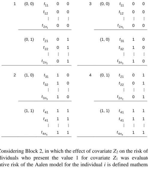
Table 1. Blocks formed by fixing one of the covariates at one of its two possible values Block Parcel Time Z1 Z2 Block Parcel Time Z1 Z2

1 (0, 0) t₁₁ 0 0 3 (0, 0) t₁₁ 0 0 t₁₂ 0 0 t₁₂ 0 0 ⁞ ⁞ ⁞ ⁞ ⁞ ⁞ t2n₁ 0 0 t2n₁ 0 0 (0, 1) t₂₁ 0 1 (1, 0) t₃₁ 1 0 t₂₂ 0 1 t₃₂ 1 0 ⁞ ⁞ ⁞ ⁞ ⁞ ⁞ t _n 2 2 0 1 t3n₃ 1 0 2 (1, 0) t₃₁ 1 0 4 (0, 1) t₂₁ 0 1 t₃₂ 1 0 t₂₂ 0 1 ⁞ ⁞ ⁞ ⁞ ⁞ ⁞ t _n 3 3 1 0 t2n2 0 1 (1, 1) t₄₁ 1 1 (1, 1) t₄₁ 1 1 t₄₁ 1 1 t₄₁ 1 1 ⁞ ⁞ ⁞ ⁞ ⁞ ⁞ t _n 4 4 1 1 t4n4 1 1

Considering Block 2, in which the effect of covariate Z2 on the risk of failure for individuals who present the value 1 for covariate Z1 was evaluated, the cumulative risk of the Aalen model for the individual i is defined mathematically by

( )

( )

( )

( )

Bl2 0 1 2 2 Λ _i t =B t +B t +B t z_i (11) In other words,

( )

( )

( )

Bl2 0 2 2 Λ _i t =B t +B t z_i (12) where B₀

( )

t =B₀

( )

t +B₁

( )

t is the cumulative risk for an individual who assumes the value 1 for covariate Z1 and 0 for covariate Z2, that is, the cumulative risk for

an individual from parcel (1, 0); and B2(t) is the cumulative regression function which represents the effect of the covariate Z2 on the risk of failure in relation to parcel (1, 0). Thus, the cumulative risks for individuals from parcels (1, 0) and (1, 1) are described in equations (13) and (14), respectively:

( )1,0

( )

0

( )

Λ t =B t (13)

and

( )1,1

( )

0

( )

2

( )

Λ t =B t +B t (14)

From the difference between the risk functions given by equations (13) and (14), the cumulative regression function B2(t) was obtained as the following equation:

( )1,1

( )

( )1,0

( )

2

( )

Λ t −Λ t =B t (15)

Equation (15) indicates the cumulative regression function B2(t) corresponds to the additional cumulative risk of individuals from parcel (1, 1) in relation to individuals from parcel (1, 0), that is, the additional cumulative risk of failure when

Z2 goes from “stage 0” to “stage 1”, for Z1 fixed at 1.

By differentiating equation (11), the instantaneous regression function of Block 2, β2(t), which is interpreted as the additional instantaneous risk of individuals from parcel (1, 1) in relation to individuals from parcel (1, 0), was obtained. In other words, the additional instantaneous risk of failure when the covariate Z2 goes from “stage 0” to “stage 1” for Z1 fixed at 1.

Similarly, the procedure was repeated for the other blocks. The cumulative regression function for each one of them was obtained from the difference between the cumulative risks of parcels from the block; that is, the additional cumulative risk when the covariate changes stage. In this way, it was verified that the cumulative regression function evaluates how much larger the cumulative risk of individuals from one parcel in comparison to the cumulative risk of individuals from another parcel. By differentiating the difference between cumulative risks of parcels from each block, the risk of instantaneous failure of one group (parcel) in relation to another group was obtained. Therefore, estimation of instantaneous risk of failure of one group (parcel) in relation to another is the estimation of the instantaneous regression function. To accomplish this, it is enough to estimate the

cumulative risk of the two groups and perform the mathematical differentiation of the difference between them, if a mathematical expression is known for the cumulative risks of these groups.

Because in the Aalen model there is no analytical expression for the cumulative risk functions of parcels as the model is non-parametric, it is appropriate to set a parametric model for each parcel. Assuming that, for each one of the parcels of one block a Weibull model can be adjusted and the cumulative risk for the individuals of each of them will be expressed by the equation

( )

Λ t t     =    

These Weibull cumulative risk functions constitute the smoothing of the cumulative regression functions of the Aalen model. Therefore, the mathematical differentiation of Weibull cumulative risk functions is the smoothing of the instantaneous risk functions of the Aalen model. According to this procedure and considering the difference between the Weibull instantaneous risks of parcels, the additional instantaneous risk of the Aalen model of a parcel in relation to another parcel was estimated. In this case, considering for example Block 2, the expression for the instantaneous regression function β2(t) is represented in equation (16):

( )

1 0 0 1 1 1 0 1 2 1 0 β t _ t _ t   − − = − (16)

where γ1, α1 are the parameters of the Weibull distribution for individuals from parcel (1, 1) and γ0, α0 are the parameters of the Weibull distribution for individuals from parcel (1, 0), respectively. Due to limitations in the estimation process of the Aalen model, the estimations for the cumulative regression functions (B) and for the instantaneous regression functions β (equations (15) and (16)) are only possible in the time range [0, τ].

Extension to Several Dichotomous Covariates of the Instantaneous Risk Function Method of Estimation of the Aalen Model

If the data set contains three dichotomized covariates, Z1, Z2, and Z3, individuals would be grouped into 23 = 8 parcels according to the triple (zi1, zi2, zi3), that is,

expression for the cumulative risk of the Aalen model for each individual with these specifications will be given as the expression (17):

( )

0

( )

1

( )

1 2

( )

2 3

( )

3

Λ_i t =B t +B t z_i +B t z_i +B t z_i (17) with B0 being the cumulative risk for an individual from parcel (0, 0, 0) and B1, B2, and B3 the cumulative regression functions that assess the effect of covariates Z1,

Z2, and Z3, respectively, at the risk of failure.

The effect of a covariate on the cumulative risk is observed by forming blocks. Thus, fixing two of the three covariates at one of its two possible values (0 or 1), individuals might be grouped into 22× 3 = 12 blocks of two parcels each. Thus, in each block, the effect of one of three covariates on the risk of failure will be evaluated for fixed values of the other two covariates. For example, Block 1 will be formed by parcels (0, 0, 0) and (0, 0, 1) and, in this block (Block 1), the effect of covariate Z3 on the risk of failure of individuals who will assume value 0 for covariates Z1 and Z2 will be assessed. Block 2 will be formed by parcels (0, 1, 0) and (0, 1, 1) and, in it (Block 2), the effect of covariate Z3 on the risk of failure of individuals who take on value 0 for covariate Z1 and value 1 for covariate Z2 will be evaluated, and so on.

In each block, considering the difference between the cumulative risks of parcels, it is possible to obtain the cumulative regression function, which will represent the additional cumulative risk for individuals from one parcel in relation to another. The mathematical differentiation (slope) of this difference provides an expression for the estimate of the instantaneous regression function. Similar to the case of two covariates, by obtaining a parametric adjustment for each parcel it will be possible to estimate the additional instantaneous risk for individuals from one parcel in relation to the instantaneous risk for individuals from another parcel.

The larger the number of covariates, the larger the number of parcels and, consequently, more blocks might be formed. The methodology described above can be used in a database with n dichotomized covariates, Z1, Z2,…, Zn–1, Zn, for a total

of 2n parcels and n× 2n–1 blocks. The blocks will be formed by fixing n – 1 covariates at one of the values 0 or 1. For each of the two parcels of each block, the non-parametric estimate for the cumulative risk can be obtained. If it is possible to obtain a parametric adjustment for each of the parcels, there will be a mathematical expression for the non-parametric cumulative risk, which will correspond to a smoothing of this risk, making it possible to estimate the instantaneous regression function of the Aalen model.

Consider a situation involving multiple covariates and consider the block in which all covariates except Z1 are fixed at 1. This block will be formed by parcels (0, 1, 1,…, 1) and (1, 1, 1,…, 1). The expressions of the Aalen model for these parcels are, respectively, described as follows:

(0,1,1, ,1)

( )

0

( )

2

( )

3

( )

( )

Λ _K t =B t +B t +B t + +K B_n t (18) and

(1,1,1, ,1)

( )

0

( )

1

( )

2

( )

3

( )

( )

Λ _K t =B t +B t +B t +B t + +K B_n t (19) The difference between the two previous expressions yields

(1,1,1, ,1)

( )

(0,1,1, ,1)

( )

1

( )

Λ _K t −Λ _K t =B t (20)

Then, there is an estimate of the additional cumulative risk for individuals from parcel (1, 1, 1,…, 1) in relation to individuals from parcel (0, 1, 1,…, 1). By obtaining a parametric adjustment for each parcel (0, 1, 1,…, 1) and (1, 1, 1,…, 1), it will be possible to estimate the additional instantaneous risk of parcel (1, 1, 1,…, 1) in relation to parcel (0, 1, 1,…, 1).

With two covariates, the estimation of the cumulative regression functions (B) (equation (19)) and of the instantaneous regression functions (β) are only

possible in the time interval [0, τ]. Given the discussion above, the purpose of this work can be used for data with a lot of dichotomous covariates.

Simulation Study

With the purpose of illustrating the methodology described in this work, two dichotomized covariates named Z1 and Z2 and individuals grouped into four sets named parcels according to the pairs (zi1, zi2): (0, 0), (0, 1) (1, 0) (1, 1) were

considered. For each of these parcels, failure times and censoring times (right censoring) were generated according to a Weibull distribution, assuming an average ratio of 30% of censorship, using the R software. The computer program can be obtained in Giarola (2009). The choice of a Weibull distribution is due to the fact that its risk function shows a behavior strictly increasing for γ > 1. Besides, this distribution has numerous applications in survival analysis. The simulation was

performed by parcel because the intention was to obtain a parametric adjustment for data of each parcel.

To observe the effect of a covariate on the risk of the Aalen model, four blocks of two parcels each were formed, fixing one of the covariates at one of its two possible values, as shown in Table 1.

The parameters of the Weibull distribution in each parcel were selected in order to obtain significance for the covariate of interest in each block of the Aalen model. The parametric values used in the Monte Carlo simulation are described in

Table 2.

Results

For each block, the cumulative risks of the Aalen model were estimated considering the distribution of data to be unknown. Subsequently, well-known cumulative risk functions that best fit the cumulative risks of the Aalen model were sought, and the difference between these well-known cumulative risk functions was determined. An instantaneous risk function for the Aalen model was obtained from the differentiation of the previous mathematical difference, as described in the Methodology section.

The results of the Aalen model adjusted to each set of blocks are shown in

Table 3, and they show that, in Block 1 at time t = τ = 7.766538, the covariate Z2 presented statistical significance, indicating that, at this time, this covariate influenced the risk of occurrence of the event, fixing the value of covariate Z1 at zero. Similar to the other blocks, it was interpreted that the respective covariates influenced the risk of occurrence of the event while maintaining the other covariate fixed.

Table 2. Sample sizes (n) and parameters of the Weibull distribution (α: scale parameter,

γ: order parameter) proposed to simulate the lifetime data, considering 30% of censorship Parcel n α γ (0, 0) 90 8.5 1.5 (0, 1) 42 4.0 2.2 (1, 0) 82 4.5 2.0 (1, 1) 64 2.0 3.5

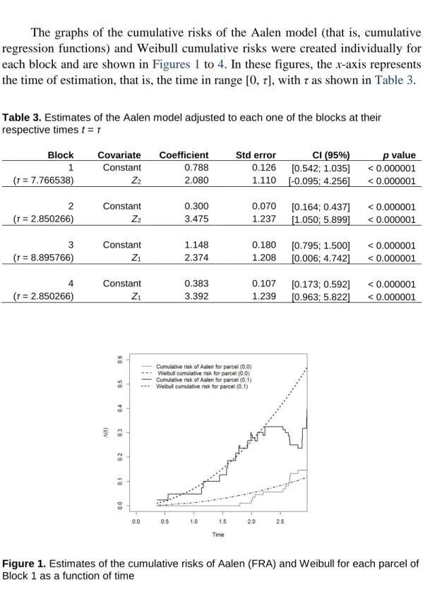
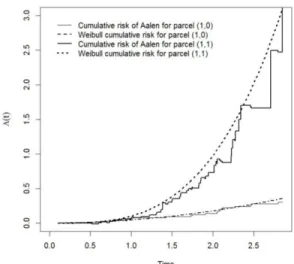
The graphs of the cumulative risks of the Aalen model (that is, cumulative regression functions) and Weibull cumulative risks were created individually for each block and are shown in Figures 1 to 4. In these figures, the x-axis represents the time of estimation, that is, the time in range [0, τ], with τ as shown in Table 3.

Table 3. Estimates of the Aalen model adjusted to each one of the blocks at their

respective times t = τ

Block Covariate Coefficient Std error CI (95%) p value

1 Constant 0.788 0.126 [0.542; 1.035] < 0.000001 (τ = 7.766538) Z2 2.080 1.110 [-0.095; 4.256] < 0.000001 2 Constant 0.300 0.070 [0.164; 0.437] < 0.000001 (τ = 2.850266) Z2 3.475 1.237 [1.050; 5.899] < 0.000001 3 Constant 1.148 0.180 [0.795; 1.500] < 0.000001 (τ = 8.895766) Z1 2.374 1.208 [0.006; 4.742] < 0.000001 4 Constant 0.383 0.107 [0.173; 0.592] < 0.000001 (τ = 2.850266) Z1 3.392 1.239 [0.963; 5.822] < 0.000001

Figure 1. Estimates of the cumulative risks of Aalen (FRA) and Weibull for each parcel of

Figure 2. Estimates of cumulative risks of Aalen (FRA) and Weibull for each parcel of Block 2 as a function of time

Figure 3. Estimates of cumulative risks of Aalen (FRA) and Weibull for each parcel of

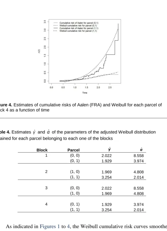
Figure 4. Estimates of cumulative risks of Aalen (FRA) and Weibull for each parcel of Block 4 as a function of time

Table 4. Estimates γˆ and αˆ of the parameters of the adjusted Weibull distribution

obtained for each parcel belonging to each one of the blocks

Block Parcel γˆ α ˆ 1 (0, 0) 2.022 8.558 (0, 1) 1.929 3.974 2 (1, 0) 1.969 4.808 (1, 1) 3.254 2.014 3 (0, 0) 2.022 8.558 (1, 0) 1.969 4.808 4 (0, 1) 1.929 3.974 (1, 1) 3.254 2.014

As indicated in Figures 1 to 4, the Weibull cumulative risk curves smoothed the cumulative risk curves for the Aalen model and the cumulative risks for individuals from parcel (1, 1) are greater than the cumulative risks for individuals from parcel (1, 0) and (0, 1). In Figure 1, it can be observed that the cumulative risks for individuals from parcel (0, 1) are greater than the cumulative risks for individuals from parcel (0, 0) after t = 2, approximately.

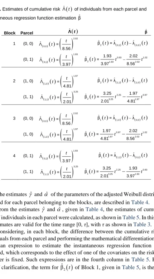
Table 5. Estimates of cumulative risk Λˆ( )t of individuals from each parcel and instantaneous regression function estimation βˆ

Block Parcel Λˆ( )t β ˆ 1 (0, 0) ˆ_{( )}( )t

( )

t 2.02 0,0 Λ = 8.56 ( ) ( )( ) ( )( ) ˆ _t ˆ _{t −}ˆ _t 2 0,1 0,0 β = λ λ (0, 1) ˆ_{( )}( )_t

( )

t 1.93 0,1 Λ = 3.97 ( ) ˆ _{t t}0.93_{− t}1.02 2 1.93 2.02 1.93 2.02 β = 3.97 8.56 2 (1, 0) ˆ_{( )}( )t

( )

t 1.97 1,0 Λ = 4.81 ( ) ( )( ) ( )( ) ˆ _t ˆ _{t −}ˆ _t 2 1,1 1,0 β = λ λ (1, 1) ˆ_{( )}( )_t

( )

t 3.25 1,1 Λ = 2.01 ( ) ˆ _{t t}2.25_{− t}0.97 2 3.25 1.97 3.25 1.97 β = 2.01 4.81 3 (0, 0) ˆ_{( )}( )t

( )

t 2.02 0,0 Λ = 8.56 ( ) ( )( ) ( )( ) ˆ _t ˆ _{t −}ˆ _t 1 1,0 0,0 β = λ λ (1, 0) ( )( )

( )

ˆ _t t 1.97 1,0 Λ = 4.81 ( ) ˆ _{t t}0.97_{− t}1.02 1 1.97 2.02 1.97 2.02 β = 4.81 8.56 4 (0, 1) ˆ_{( )}( )t

( )

t 1.93 0,1 Λ = 3.97 ( ) ( )( ) ( )( ) ˆ _t ˆ _{t −}ˆ _t 1 1,1 0,1 β = λ λ (1, 1) ( )( )

( )

ˆ _t t 3.25 1,1 Λ = 2.01 ( ) ˆ _{t t}2.25 _{− t}0.93 1 3.25 1.93 3.25 1.93 β = 2.01 3.97

The estimates ˆ and ˆ of the parameters of the adjusted Weibull distribution, obtained for each parcel belonging to the blocks, are described in Table 4.

From the estimates ˆ and ˆ , given in Table 4, the estimates of cumulative risks of individuals in each parcel were calculated, as shown in Table 5. In this table, the estimates are valid for the time range [0, τ], with τ as shown in Table 3.

Considering, in each block, the difference between the cumulative risks of individuals from each parcel and performing the mathematical differentiation of the result, an expression to estimate the instantaneous regression function β was obtained, which corresponds to the effect of one of the covariates on the risk when the other is fixed. Such expressions are in the fourth column in Table 5. For the sake of clarification, the term for ˆβ₂

( )

t of Block 1, given in Table 5, is the effect

of the covariate Z2 on the risk by fixing Z1 at zero, and the expression for ˆβ₂

( )

t of Block 2 corresponds to the effect of covariate Z2 on the risk by fixing Z1 at 1.

The graphs for the estimates of these instantaneous regression functions versus time are shown in Figures 5 to 8.

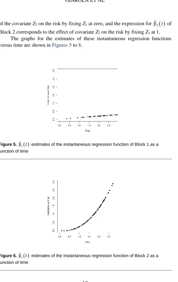
Figure 5. βˆ₂( )t estimates of the instantaneous regression function of Block 1 as a

function of time

Figure 6. βˆ₂( )t estimates of the instantaneous regression function of Block 2 as a

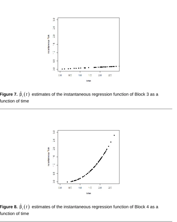
Figure 7. βˆ₁( )t estimates of the instantaneous regression function of Block 3 as a function of time

Figure 8. βˆ₁( )t estimates of the instantaneous regression function of Block 4 as a

function of time

As indicated in these graphs, the instantaneous risk of individuals from parcel (1, 1) is larger than the instantaneous risk of individuals from parcels (0, 1) and (1, 0), and these last two are greater than the instantaneous risks of individuals from parcel (0, 0). Finally, the difference between the instantaneous risks of the parcels

is increasing. In Figure 5 at t = 2, for example, approximately ˆβ 0.203₂ = was obtained. This means that, at t = 2, in a given unit of time previously defined (days, months, years,…), an average of 0.203 failures would happen, which corresponds to 1 failure for every 4.93 units of time (1 / 0.203 = 4.93), on average. Thus, individuals from parcel (0, 0) need, on average, 4.93 units of time more than individuals from parcel (0, 1) to experience the event. Similar interpretations might be made from Figures 6 to 8. All results and simulation data were obtained using the R software (R Development Core Team, 2009).

Conclusion

The estimation process proposed for the Aalen model is only possible in the time range [0, τ], that is, when X(t)ˈX(t) is non-singular. This restriction also applies to the methodology proposed here, because it is based on the Aalen model. Thus, the estimation of the instantaneous risk function of the Aalen model for dichotomous covariates using parametric smoothing is also only possible for t in the range [0, τ]. The proposed method can be used with many dichotomous covariates. However, if the number of covariates increases, the number of parcels and blocks increases considerably and the number of individuals per parcel decreases, which can make estimation in the parcels impossible.

Parcels with large sample sizes (greater than 40) and an average ratio of censorship of 30%, according to Table 2, were considered. Thus, failure and censoring times were generated according to the Weibull distribution. The simulation was performed per parcel, allowing different parametric forms to be assumed for each parcel. The choice of the value 30% for the proportion of censoring is because it is a high value and, thus, it is a worse situation than the one in which the proportion of censorship is smaller.

Although situations in which there is a mix of different kinds of covariates (dichotomous, continuous, and polytomic) are common, there are also situations in which there are only dichotomous covariates. One of these situations was presented by Grunkemeier et al. (2006). The authors compared the effect of two treatments on the risk of some diseases. The treatments consisted in implanting one of two heart valve types. The effect of the use of a valve type (Silzone valve), in relation to the effect of another type of valve (control valve), on the risk of failure was evaluated considering the Aalen model and using the Gompertz distribution to smooth the cumulative risk functions of this model. In this case, there was only a dichotomous covariate: type of valve (Silzone or control). There are also situations

in which one wishes to determine the effect of using two medications on the risk of cure of a disease, and some patients are treated with only one medication while others are treated simultaneously with both. In this case, there are two dichotomous covariates, one for each medication. An example of this was presented by Giarola (2009). The author used the Lognormal distribution to smooth the cumulative risk function. This fact emphasizes the use of other parametric distributions besides the Weibull one.

In the presence of dichotomous covariates, the functions of cumulative risk of the Aalen model can be adjusted by well-known cumulative risk functions, allowing the estimation of the instantaneous risk of the Aalen additive model of a group in relation to another by stratification of data in parcels. The methodology can be used for data with many dichotomous covariates. However, it is noteworthy that the higher the number of covariates, the greater the number of parcels and the smaller the number of individuals per parcel.

References

Aalen, O. (1978). Nonparametric inference for a family of counting processes. The Annals of Statistics, 6(4), 701-726. doi: 10.1214/aos/1176344247

Aalen, O. (1980). A model for nonparametric regression analysis of counting processes. In W. Klonecki, A. Kozek, & J. Rosiński (Eds.),

Mathematical statistics and probability theory (pp. 1-25). doi: 10.1007/978-1-4615-7397-5_1

Aalen, O. O. (1989). A linear regression model for the analysis of life times.

Statistics in Medicine, 8(8), 907-925. doi: 10.1002/sim.4780080803

Aalen, O. O. (1993). Further results on the non-parametric linear regression model in survival analysis. Statistics in Medicine, 12(1), 1569-1588. doi:

10.1002/sim.4780121705

Aydemir, S., & Biller, C. (1997). Kernel smoothing of Aalen’s linear regression model (Sonderforschungsbereich 386, Paper 101). Munich, Germany: Ludwig Maximilian University of Munich Institute of Statistics. doi:

10.5282/ubm/epub.1491

Başar, E. (2017). Aalen's additive, Cox proportional hazards and the Cox-Aalen model: Application to kidney transplant data. Sains Malaysiana, 46(3), 469-476. doi: 10.17576/jsm-2017-4603-15

Carvalho, M. S., Andreozzi, V. L., Codeço, C. T., Barbosa, M. T. S., & Shimakura, S. E. (2005). Análise de sobrevida: Teoria e aplicações em saúde

[Survival analysis: Health theory and applications] (2nd ed.). Rio de Janeiro, Brazil: FIOCRUZ. doi: 10.7476/9788575413029

Fahrmeir, L., & Tutz, G. (1996). Multivariate statistical modelling based on generalized linear models. New York: Springer-Verlag. doi: 10.1007/978-1-4899-0010-4

Fleming, T. R., & Harrington, D. P. (1991). Counting processes and survival analysis. New York, NY: J. Wiley.

Fogo, J. C. (2007). Modelo de regressão para um processo de renovação Weibull com termo de fragilidade [Regression model for a Weibull renewal process distribution with a frailty effect] (Doctoral dissertation). Luiz de Queiroz College of Agriculture, Piracicaba, Brazil.

Gandy, A., & Jensen, U. (2005). On goodness-of-fit for Aalen’s additive risk model. Scandinavian Journal of Statistics, 32(3), 425-445. doi:

10.1111/j.1467-9469.2005.00457.x

Giarola, L. T. P. (2009). Extensão para várias covariáveis do método de estimação da função de risco instantâneo do modelo aditivo de Aalen [Extension for several covariates of the method of estimation of the instantaneous risk function of the additive model of Aalen] (Doctoral dissertation). Federal University of Lavras, Lavras, Brazil. Retrieved from

http://repositorio.ufla.br/jspui/handle/1/4403

Grunkemeier, G. L., Jin, R., Im, K., Holubkov, R., Kennard, E. D., & Schaff, H. V. (2006). Time-related risk of St. Jude Silzone heart valve. European Journal of Cardio-Thoracic Surgery, 30(1), 20-27. doi:

10.1016/j.ejcts.2006.04.012

Henderson, R., & Milner, A. (1991). Aalen plots under proportional hazards.

Journal of the Royal Statistical Society. Series C (Applied Statistics), 40(3), 401-409. doi: 10.2307/2347520

Keiding, N., & Andersen, P. K. (1989). Nonparametric estimation of transition intensities and transition probabilities: A case study of a two-state Markov process. Journal of the Royal Statistical Society. Series C (Applied Statistics), 38(2), 319-329. doi: 10.2307/2348062

Lima, L. V. (2007). Métodos clássicos e bayesianos de estimação da janela ótima em núcleo-estimadores [Classical and Bayesian methods of estimation of optimal window in core-estimators] (Master’s thesis). Federal University of

Minas Gerais, Belo Horizonte, Brazil. Retrieved from

http://www.bibliotecadigital.ufmg.br/dspace/handle/1843/RFFO-7KMQ4T

Lin, D. Y., & Ying, Z. (1994). Semiparametric analysis of the additive risk model. Biometrika, 81(1), 61-71. doi: 10.1093/biomet/81.1.61

Ma, S., Kosorok, M. R., & Fine, J. P. (2006). Additive risk models for survival data with high-dimensional covariates. Biometrics, 62(1), 202-210. doi:

10.1111/j.1541-0420.2005.00405.x

Mansourvar, Z. & Martinussen, T. (2017). Estimation of average causal effect using the restricted mean residual lifetime as effect measure. Lifetime Data Analysis, 23(3), 426-438. doi: 10.1007/s10985-016-9366-z

Martinussen, T., & Scheike, T. H. (2009). The additive hazards model with high-dimensional regressors. Lifetime Data Analysis, 15(3), 330-342. doi:

10.1007/s10985-009-9111-y

Mau, J. (1986). On a graphical method for the detection of time-dependent effects of covariates in survival data. Journal of the Royal Statistical Society. Series C(Applied Statistics), 35(3), 245-255. doi: 10.2307/2348023

Pereira, T. L. (2004). Modelo de riscos proporcionais e aditivos para o tratamento de covariáveis dependentes do tempo [Proportional and additive risk models for the treatment of time-dependent covariates] (Master’s thesis). Federal University of Pernambuco, Recife, Brazil. Retrieved from

https://repositorio.ufpe.br/handle/123456789/6590

R Development Core Team. (2009). R: A language and environment for statistical computing [computer software]. Vienna, Austria: R Foundation for Statistical Computing. Retrieved from https://www.r-project.org/

Ramlau-Hansen, H. (1983). Smoothing counting process intensities by means of kernel functions. The Annals of Statistics, 11(2), 453-466. doi:

10.1214/aos/1176346152

Silverman, B. W. (1986). Density estimation of statistics and data analysis. London, UK: Chapman and Hall.