1 INTRODUCTION
Testing is one of the key factors to any software products’ success and data warehouse systems are no exception. Data warehouse can be tested in different ways (e.g. front-end testing, database testing) but testing the data warehouse’s ETL procedures (sometimes called back-end testing [1]) is probably the most complex and critical data warehouse testing job, because it directly affects the quality of data. Throughout the ETL process, source data is being put through various transformations, from simple algebraic operations to complex procedural modifications. The question is how accurate and reliable is data in the data warehouse after passing through all these transformations and, in the first place, have the data
that should have been extracted actually been extracted and subsequently transformed and loaded?
In order to attain a certain degree of confidence in the data quality, series of test should be performed on a daily basis. Like any software system, data warehouse’s ETL system can be tested in various fashions, for instance, one can test small isolated ETL components using unit tests or one can test the overall process using integration tests (not to mention other kinds of testing like regression tests, system tests etc. [2]).
In this paper we propose a generic procedure for (back-end) integration testing of certain aspects of ETL procedures. More precisely, we’re interested in asserting whether all data is accurately transferred throughout the ETL process, that is whether “all counts match”. ETL In order to attain a certain degree of confidence in the quality of the data in the data warehouse it is necessary to perform a series of tests. There are many components (and aspects) of the data warehouse that can be tested, and in this paper we focus on the ETL procedures. Due to the complexity of ETL process, ETL procedure tests are usually custom written, having a very low level of reusability. In this paper we address this issue and work towards establishing a generic procedure for integration testing of certain aspects of ETL procedures. In this approach, ETL procedures are treated as a black box and are tested by comparing their inputs and outputs – datasets. Datasets from three locations are compared: datasets from the relational source(s), datasets from the staging area and datasets from the data warehouse. Proposed procedure is generic and can be implemented on any data warehouse employing dimensional model and having relational database(s) as a source.
Our work pertains only to certain aspects of data quality problems that can be found in DW systems. It provides a basic testing foundation or augments existing data warehouse system’s testing capabilities. We comment on proposed mechanisms both in terms of full reload and incremental loading.
Key words: data quality, data warehouse, dimensional model, ETL testing
Croatian translation of the title. Općeniti postupak za integracijsko testiranje ETL procedura
Kako bi se ostvarila odreñena razina povjerenja u kvalitetu podataka potrebno je obaviti niz provjera. Postoje brojne komponente (i aspekti) skladišta podataka koji se mogu testirati. U ovom radu smo se usredotočili na testiranje ETL procedura. S obzirom na složenost sustava skladišta podataka, testovi ETL procedura se pišu posebno za svako skladište podataka i rijetko se mogu ponovo upotrebljavati. Ovdje se obrañuje taj problem i predlaže općenita procedura za integracijsko testiranje odreñenih aspekata ETL procedura. Predloženi pristup tretira ETL procedure kao crnu kutiju, te se procedure testiraju tako što se usporeñuju ulazni i izlazni skupovi podataka. Usporeñuju se skupovi podataka s tri lokacije: podaci iz izvorišta podataka, podaci iz konsolidiranog pripremnog područja te podaci iz skladišta podataka. Predložena procedura je općenita i može se primijeniti na bilo koje skladište podatka koje koristi dimenzijski model pri čemu podatke dobavlja iz relacijskih baza podataka. Predložene provjere se odnose samo na odreñene aspekte problema kvalitete podataka koji se mogu pojaviti u sustavu skladišta podataka, te služe za uspostavljanje osnovnog skupa provjera ili uvećanje mogućnosti provjere postojećih sustava. Predloženi postupak se komentira u kontekstu potpunog i inkrementalnog učitavanja podataka u skladište podataka.
Ključne riječi: kvaliteta podataka, skladište podataka, dimenzijski model, testiranje ETL-a Igor Mekterović, Ljiljana Brkić, Mirta Baranović
A Generic Procedure for Integration Testing of ETL
Procedures
UDK xxx.xxx.xx
IFAC x.x;x.x.x (filled by editors)
procedures are tested as a whole since we only compare inputs and outputs of ETL procedures: datasets. Namely, we compare the data from relational data sources with the data integrated at the staging area and finally with the data stored in a dimensional model (we assume that data warehouse employs dimensional model). In order to do so, it must be possible to trace each record back to its source, or establish data lineage. In a warehousing environment, asserting data lineage is defined as (back)tracing warehouse data items back to the original source items from which they were derived [3].
We propose an easy to implement data lineage mechanism and upon it we build procedures for comparing datasets. Requiring only small interventions to the ETL process, proposed procedure can be elegantly implemented on the existing DW systems. The intention is to treat this testing procedure as an addition to the ETL process that will provide more insight into the quality of the data. Our work pertains only to certain aspects of data quality.
Data quality is considered through various dimensions and the data quality literature provides a thorough classification of data quality dimensions. However, there are a number of discrepancies in the definition of most dimensions due to the contextual nature of quality [4]. There is no general agreement either on which set of dimensions defines the quality of data, or on the exact meaning of each dimension [4]. However, in terms of most agreed upon and cited data quality dimensions [5], our work pertains to accuracy (sometimes called precision) and reliability (free-of-error). In this context, we do not consider data quality issues between real world and relational database, but between relational database and data warehouse. In that sense, inaccuracy would imply that data warehouse system represents a source system (relational databases) state different from the one that should be represented [5]. We consider reliability as “the extent to which data is correct and reliable” [4] and “whether can be counted upon to convey the right information” [5].
Described procedure is being implemented in Higher Education Information System Data Warehouse in Croatia [6]. The rest of this paper is structured as follows. In section 2, related work is presented. Section 3 describes the architecture of the proposed testing system. In Section 4 we examine how to establish data lineage in systems that employ dimensional model and formally describe the proposed solution. Section 5 introduces the segmenting procedure used to find discrepancies between two data sets. Sections 6 and 7 describe counting and diff subsystem used to compare record counts from data sources, staging area and dimensional model structures and pinpoint excess or missing records. Section 8 describes preliminary results. Finally, Section 9 presents
our conclusions.
2 RELATEDWORK
Data quality is of major concern in all areas of information resources management. A general perspective on the data quality is given in [7] [8]. Data quality issues in a data warehousing environment are studied in [9] [10]. Properties of data quality are analyzed through a set of data quality dimensions. A vast set of data quality dimensions is given in [5] [4] [9]. Practical aspects of data quality, including data quality dimensions, methodology for their measurement and improvement, can be found in [11] [12].
An overall theoretical review and classification of data warehouse testing activities is given in [1]. The difference between data warehouse testing and normal testing is emphasized, and phases of data warehouse testing are discussed. In [13] regression testing ETL software is considered and a semi-automatic regression testing framework is proposed. Proposed framework is used to compare data between ETL runs to catch new errors when software is updated or tuned. On the contrary we test and compare data at different points within a single ETL run.
Besides regression and integration testing, there are various tools and frameworks for unit testing ETL procedures [14][15]. A number of papers [16] [17] [18] proposes strategies and models for generation of data quality rules and their integration into ETL process.
Establishing data lineage (or data provenance) is tightly related to the testing of the outcomes of the ETL procedures. Data lineage can be described in different ways depending on where it is being applied (in context of database systems, in geospatial information systems, in experiment workflows,…) [19]. The problem of establishing data lineage in data warehousing environments having relational database as a data source has been formally studied by Cui et al. in [3] [20]. In [21] is stated that embedding data lineage aspects into the data flow and workflow can lead to significant improvements in dealing with DQ issues and that data lineage mechanism can be used to enable users to browse into exceptions and analyze their provenance.
Although there are various commercial and scientific efforts in the ETL testing area, our work is, to the best of our knowledge, the first to provide a generic procedure for integration testing of the ETL procedures.
3 THEARCHITECTUREOFTESTINGSYSTEM
Due to the complexity and domain differences, it is hard if not impossible to develop an automated testing tool that will test warehouse data and ETL procedures. It is true that ETL have been somewhat standardized in the
last years, but certainly not to the extent that would allow for such testing tools. After all, ETL procedures differ in architectural and technological sense. Therefore, to fully test the data and ETL procedures, custom tests and queries have to be written.
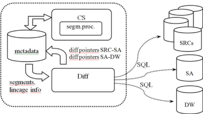
We propose (Figure 1) a procedure that will test warehouse data (DW) versus data consolidated in staging area (SA) and versus data from (relational) sources (SRC). The proposed procedure can be applied to existing data warehouse systems having minimal impact on the existing ETL procedures.
Figure 1. The architecture of the testing system The procedure relies on a metadata describing sources, staging area and data warehouse and performs two tasks:
• checks for differences in record counts (we refer to this part as the “counting subsystem” or “CS”)
• finds and maintains identifiers to unsynchronized records (we refer to this part as the “diff subsystem” or “DS”)
In order to introduce this generic procedure certain assumptions have to be made. Firstly, it is expected for the data warehouse to employ dimensional data model [22] having data organized in fact and dimensional tables (even though, when revised, this procedure could work with other data models). Secondly, every record in the fact table must be traceable to the single source record (lineage) and vice versa (dependency). Obviously, this leaves out aggregated tables, snapshots, etc. Implementation-wise, this means that it must be possible to trace and store matching unique identifiers. In order to achieve this, minor modifications to the existing ETL procedures will have to be made. Finally, we assume that each dimension table record holds a business (relational) key, thus maintaining a back reference to the source data.
As mentioned, proposed procedure relies on metadata that describes existing structures. Metadata describes relational sources and tables, staging area tables, dimension model tables and their mappings. Due to the space limitations, we shall not describe metadata tables in detail, but shall, at places, bring to attention certain information that needs to be stored in metadata repository.
4 ESTABLISHINGTHEDATELINEAGE
In this section we examine how to establish data lineage in systems that employ dimensional model and formally describe the proposed solution.
Although our goal is to introduce data lineage capabilities to existing systems with as little intrusion as possible, certain changes will have to be made to establish lineage and dependency between source and data warehouse data. Setting up the lineage of dimensional data is pretty straightforward since dimension table schemas usually include business (relational) key, thus maintaining a back reference to the source data. If not, this key should be added in lines with the best design practices. We propose the following procedure for tracking data lineage of dimension tables.
Let be the schema of the consolidated source table :
, … , , , …
where is the business key attribute and is the dependent attribute. Shorter, we denote a consolidated source table schema:
,
Consolidated source table contains data from different sources after being cleaned, integrated and deduplicated. Such source table, enriched with other consolidated source tables (e.g. joined with related tables), can serve as a foundation for either dimensional or fact table.
Let be the schema of the dimension table : , ,
where is a surrogate identity key (auto incrementing integer), is an attribute set taken from , is a set of dependent dimensional attributes.
Differences between source and dimension table consist of two record sets given with the following expressions:
1. Tuples that exist in the source and don't exist in the destination table
π
\π
>>>><<<<
2. Tuples that exist in the destination and don't exist in the source table:
π
\
π
>><>><<<For fact tables, on the other hand, the solution is more complex. We only consider the most common fact table type - transactional fact table, leaving out cumulative fact tables and periodic snapshots [22]. Fact tables are recoded in a way that relational foreign keys are replaced with dimension table surrogate keys.
Let be the schema of the fact table : , … , , … , where is the dimension foreign key and is the measure. Shorter, we denote fact table schema:
,
Source table records are sometimes filtered on extraction, e.g. a row could be describing an incomplete activity. For instance, an order that has been placed but not yet delivered is excluded from loading into the data warehouse pending delivery. That is why we introduce ’
σ
!"# abstraction.Let st& be the filtered source table based on ST with the same schema as ST:
&
σ
!"#To achieve fact table data lineage, we propose the following procedure that we consider to be generic and easy to implement (Figure 2).
For each fact table :
• Add ) attribute as a surrogate identity key thus changing fact table schema to:
), , • Create lineage table ! * with schema:
+ * ), , … ,
where is the business key attribute of the fact table's source table. Shorter:
+ * ),
• Prior to loading fact table, in order to generate surrogate ids, redirect data stream to table ! * ,-with schema:
+ *,- ), , ,
• Split ! *,-into two projections ! * and as follows:
! *
π
, ! *
,-π
, ,! *
,-Once lineage tables have been created and populated, queries returning excess and missing records can be generated in a generic manner for each fact table. Differences between source and fact table consist of the two sets:
1. Tuples missing from the fact table i.e. exist in the source and don't exist in the destination table:
.
π
/\π
>><>><<< ! *0>><>><<< &2. Excess tuples i.e. exist in the fact table and don't exist in the source table:
.
π
>><>><<< ! *\π
/0><>>><<< ! *>><>><<< 1π
\
π
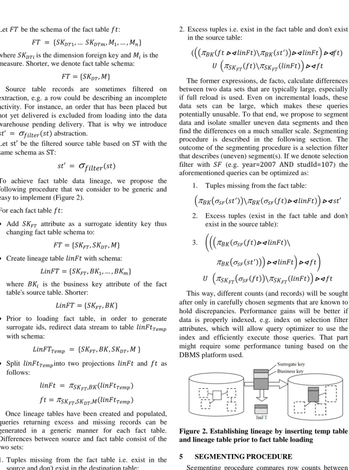
! *>><>><<<The former expressions, de facto, calculate differences between two data sets that are typically large, especially if full reload is used. Even on incremental loads, these data sets can be large, which makes these queries potentially unusable. To that end, we propose to segment data and isolate smaller uneven data segments and then find the differences on a much smaller scale. Segmenting procedure is described in the following section. The outcome of the segmenting procedure is a selection filter that describes (uneven) segment(s). If we denote selection filter with (e.g. year=2007 AND studId=107) the aforementioned queries can be optimized as:
1. Tuples missing from the fact table:
π
.σ)/0\π
σ)><>>><<< ! *>>>><<<< & 2. Excess tuples (exist in the fact table and don'texist in the source table): 3. 23
π
σ)>><>><<< ! *\π
.σ)/0>><>><<< ! *4>><>><<< 51
π
.σ)0\
π
! *>>>><<<< This way, different counts (and records) will be sought after only in carefully chosen segments that are known to hold discrepancies. Performance gains will be better if data is properly indexed, e.g. index on selection filter attributes, which will allow query optimizer to use the index and efficiently execute those queries. That part might require some performance tuning based on the DBMS platform used.Figure 2. Establishing lineage by inserting temp table and lineage table prior to fact table loading
5 SEGMENTINGPROCEDURE
Segmenting procedure compares row counts between two data sets and tries to isolate small segments of data that hold discrepancies. This is performed by grouping data and comparing matching group row counts at source
and destination. Segmenting attributes (or attribute functions, e.g. YEAR(orderDate)) for each table are defined in metadata repository. These attribute in fact define a hierarchy that is used to “drill down” when searching for discrepancies. For tables that are used as sources for fact tables, segmenting attributes are typically time related (e.g. year → month → day), since every fact table has a timestamp attribute marking the time when the
events of the process being tracked occurred (e.g. Orders table has attribute OrderDate). Also, fact table data is usually evenly distributed over timestamp attribute. This is true for most processes as it means that similar amount of data are generated in given time intervals (e.g. daily).
Consider the following example (Table 1).
Table 1 Drilling down through the time to find differences more precisely All time
→
Broken into time frames
→
Broken into time frames further more 75<>65 2007 25 != 20 ERR 2007 2008 15 = 15 Q1 5 != 0 ERR 2009 20 = 20 Q2-Q4 20=20 2010 15 != 10 ERR 2008 15 =15 2009 20 =20 2010 Jan 10 = 10 Feb 5 != 0 ERR Starting from the “all time” count, data is
consecutively broken down into smaller time frames, much like the OLAP style drill down operation, until small enough erroneous counts (segments) are isolated. Data is segmented in a greedy fashion: when uneven (in terms of row counts) segments are found they are drilled down with greater priority and full depth. Even segments are drilled down only to a certain, smaller depth. Segmenting procedure stores and maintains these counts per segments in metadata repository. Past counts can be used to facilitate future segmenting jobs since erroneous data often stays in the same segments between two checks. Also, past counts are particularly useful if incremental loading strategy is employed. Newly generated records at source dataset will have an impact only on a small number of segments (if time attributes are used for segmenting changed segments will typically be the most recent ones). With that in mind, only incremented data segments are inspected.
It must be noted that such batch count comparison does
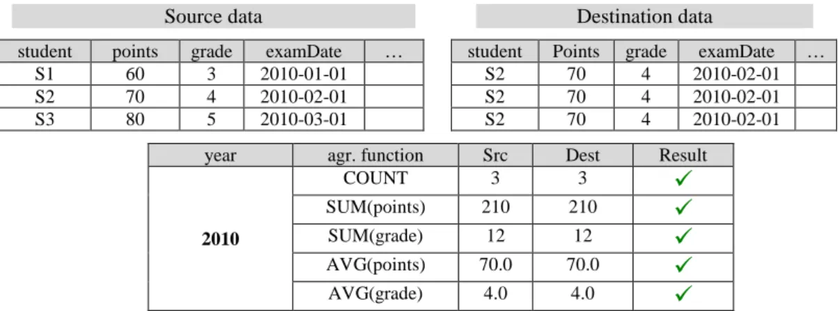
not necessarily find (all) discrepancies. It is inherently error prone – excess and missing records annul each other and if their counts match – the overall count appears correct. To reduce the possibility of error, other aggregate function values within the same queries can be checked, if developer so defines. In other words, COUNT is the default (and obligatory) function, but others can be defined on a per table basis. The obvious choice is the SUM function. However, SUM function (and all other aggregate functions besides COUNT) must be defined over a certain attribute. In a typical setup, we check for sum values of all fact table measures that are transferred unchanged from the source system. Still, these additional checks only reduce the possibility of error; Table 2 shows an example of erroneous data that, never the less, passes all these checks (ETL process erroneously discarded S1 and S3 and multiplied S2 three times). Should the segment be drilled down to month, errors would become apparent.
Table 2 . Erroneous data that passes the check on a year level
Source data Destination data
student points grade examDate … S1 60 3 2010-01-01 S2 70 4 2010-02-01 S3 80 5 2010-03-01
student Points grade examDate … S2 70 4 2010-02-01 S2 70 4 2010-02-01 S2 70 4 2010-02-01 year agr. function Src Dest Result
2010 COUNT 3 3
SUM(points) 210 210
SUM(grade) 12 12
AVG(points) 70.0 70.0
AVG(grade) 4.0 4.0
Note that segment could, in theory, be drilled down to primary key values which would compare single records. This is a useful property since it enables the segmenting procedure to be tunable – to search for errors on different levels of granularity depending on how much resource (time, hardware) is available and how much a certain fact or dimension table is important. Other aggregate
functions are less useful in this context: AVG can be regarded as SUM/COUNT. MIN and MAX help only if erroneous record is of minimal or maximal value.
6 COUNTINGSUBSYSTEM
Counting subsystem’s task is to compare record counts from data sources, staging area and dimensional model structures. Different counts indicate the segment in which errors occurred (Figure 3) – either Change Data Capture/Data extraction segment or data transformation and loading segment. Figure 3 shows both overall count and incremental counts (e.g. on last CDC load). Numbers shown in bold denote differences in counts – cumulative (3050<>3040<>3030) and on last incremental load (17=17<>16). Not all structures are populated incrementally – for those structures that are not populated incrementally, only the overall count is being observed.
Figure 3. Count comparison at three referent ETL points (storages)
In the following two sections we consider the CS with regards to two aforementioned ETL phases.
6.1 CDC/Extract phase counting subsystem
The first part of every ETL process is data extraction from, often more than one, source. In this paper, we consider only relational databases as potential sources, that is we do not consider flat files, spreadsheets, xml files, etc.(as a workaround, these other kinds of sources could be systematically parsed and loaded into relational database and thus indirectly traced). In the process of data extraction and copying (to the staging area) various errors can occur. For instance, network error can occur and prevent transfer of some subset of data. Permission errors can occur, preventing the account that performs the extraction to read all or some of the data. Further more, domain errors can occur on data insertion in the staging area, e.g. negative numbers cannot be inserted into
unsigned integer fields; date types can overflow ranges – for instance Informix’s DATE type (ranging from year 1-9999) will not fit into any Microsoft SQL Server’s DATETIME type prior to version 2008 (at best, ranging from year 1753 to 9999), etc. To calrify, althought years prior to 1753 are most likely errors that should have been caught in the users’ applications that is not the reason to omit those rows in the data warehouse – they should appear, properly flagged.
In this phase, CS checks data counts in the staging area versus source data counts. The first step of the ETL process implies mirroring relevant source tables to the staging area (where they are subsequently integrated). Each mirrored table (count) is compared to its original table (count). We consider two setups: full reload and incremental load.
Figure 4 shows a full reload setup in which data is extracted at t1 from N sources (N=2; src0 and src1) and copied to corresponding mirrored table in the staging area. Note that, even on full reload, if source systems aren’t taken offline for the duration of extraction, there should be some kind of timestamp mechanism that will enable to create a data snapshot at certain moment in time. Otherwise, it is possible to have uneven data in terms of creation date. On Figure 4 data that is created after the extraction time t1 (and is not being extracted at this ETL batch) is denoted with an empty rectangle. Immediately after the extraction, CS uses segmenting procedure and compares counts between mirrored data and source data. Obviously, segmenting attributes (hierarchies) for every table have to be defined.
Figure 4. Loading data from RDBMS sources to SA in full reload scenario
CS maintains these counts between different ETL batches. Besides comparing actual counts, CS also compares new count with previous version’s count. Typically, in every table of a database record count grows or stays the same. Therefore, ever new version should, in
principal, have more and more records. Of course, it is entirely possible for some table to reduce number of records from one ETL batch to another. That is why, for each table, we define a threshold and check whether actual record count is bigger than threshold times previous record count (Table 3). The larger the table, the closer to 1 is threshold set (e.g. 1 deleted row in table of 3 records can be a 33% drop; however in large tables such big drops are more unlikely). This mechanism provides yet another indicator of potentially bad data.
Table 3 Threshold check for table T1 and threshold t = 0.9
Load T1 count T1 prev. ver.
count Check Result #1 100 90 100 > t * 90
#2 110 100 110 > t * 100
#3 105 110 105 > t * 110
#4 50 105 50 > t * 105 ERR
On incremental loads, the same procedure is applied but in an incremental fashion. Incremental data is segmented (if possible) and counts are added to the existing count tables. Note that counts can be negative if, in a certain segment, delete operation outnumbers the insert operation. After being counted, incremental data are merged into staging area replica of the source. Optionally, to check for possible CDC errors at the source, newly computed (after merge) counts can be checked versus the source counts in all segments (which can be resource consuming with large tables) or only in segments corresponding to the last processed CDC batch. 6.2 Transform/load counting subsystem
This part of CS compares counts between consolidated data in the staging area and according dimensional model. Unfortunately, unlike previous phase, these counts (records) aren’t always related one to one. For instance,
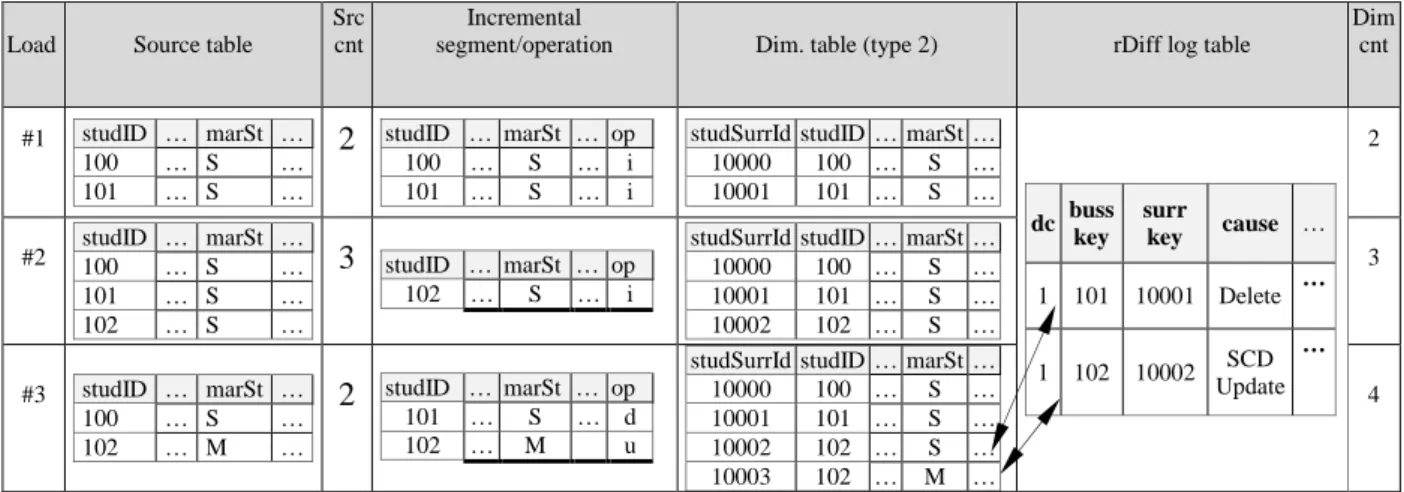
type 2 dimensions [22] have more records than underlying source data tables. With type 2 dimensions, a new record is added to the table whenever one of their type 2 attributes changes its value thus preserving history. Table 4 presents such scenario where a type 2 dimension is incrementally populated and data counts rightfully differ. Source table rows and rows detected by CDC system are shown in separate columns, along with the flag of data operation that occurred (insert, delete, update). In load #3 counts begin to rightfully differ: a student with studID=102 changes his or hers marital state – a new row is inserted with the latest marital state; previous fact records are still connected to the original dimension row with studSurrId=10002, and new fact records are connected to the new row with studSurrId=10003. These type 2 updates should be detected at integrated source system which resides in the staging area; because it is not possible to detect missing type 2 inserts in the dimensional tables that should have occurred (rightly created type 2 records can be detected using business key). Deletions can also cause situations when counts rightly differ. Depending on the data population strategy, deleted rows could also be deleted from the data warehouse, or they could be preserved (sometimes only marked as deleted). This information is stored in the metadata repository that the proposed procedure relies on. Load #3 depicts such scenario where delete operation in the source system does not cause the deletion of corresponding dimension record (studID =101). To the best of our knowledge, insert operations in the source system always cause corresponding new records in the dimensional tables (by “source system” we mean integrated source system, after data from different sources has been integrated and deduplicated, etc.).
Table 4 Regular count mismatch on incrementally populated Type-2 dimensions
Load Source table
Src cnt
Incremental
segment/operation Dim. table (type 2) rDiff log table
Dim cnt #1 studID … marSt … 100 … S … 101 … S …
2
studID … marSt … op 100 … S … i 101 … S … istudSurrId studID … marSt …
10000 100 … S … 10001 101 … S … dc buss key surr key cause … 1 101 10001 Delete … 1 102 10002 SCD Update … 2 #2 studID … marSt … 100 … S … 101 … S … 102 … S …
3
studID … marSt … op 102 … S … istudSurrId studID … marSt …
10000 100 … S … 10001 101 … S … 10002 102 … S … 3 #3 studID … marSt … 100 … S … 102 … M …
2
studID … marSt … op 101 … S … d 102 … M ustudSurrId studID … marSt …
10000 100 … S …
10001 101 … S …
10002 102 … S …
10003 102 … M …
Fact tables can also have more records than their source tables if records deletions are not carried out in the data warehouse.
Table 5 sums up the effects of CDC operations on dimensional structures. Operations shown in bold result in different counts between source and dimension tables. With type 1 dimensions, situation is simpler because update operations cause dimension records updates. Table 5. CDC operations repercussions on dimensional structures
CDC operation
Type 1 Dim. Type 2 Dim. Fact table Insert Insert Insert Insert Update Update Insert Update/None Delete Delete/None Delete/None Delete/None
In order to keep track of valid counts, identifiers of (regular) surplus rows (rDiff log table in Table 4, r stands for “regular”) have to be logged and maintained. rDiff log tables store business and surrogate keys, description as to why the record is created and affected differential record count dc (usually 1, e.g. one deleted record affects overall count with quantity 1). Of course, in existing systems such rDiff tables do not exist beforehand. rDiff log tables have to be created (and initially populated) for each relevant table as accurately possible, and rows that cannot be accounted for should be represented as single row in rDiff log table having dc > 1 and e.g. “initialization” listed as cause. Business and surrogate keys for those rows are unknown (NULL). This will enable to isolate future errors from the batch of “inherited” errors.
According to Kimball [22], there are three types of fact tables: periodic snapshots, accumulating snapshots and transactional fact tables. For the time being, we focus on the latter, the most common fact table type. Analogous issues arise as with dimensional tables so we omit further comments.
7 DIFFSUBSYSTEM
Diff subsystem’s responsibility is to pinpoint excess or missing records and maintain identifiers for those records. This task naturally follows count subsystem’s findings (Figure 5). Diff uses information about data segments and finds exact records for relevant tables. In order to find those records, Diff uses lineage mechanisms (and generates SQL queries) described in section 4.
Figure 5. Diff subsystem
Diff subsystem maintains a single iDiff (i stands for “irregular”) identifier table for each relevant table. These tables are similar to those described in the previous section, except that rDiff tables pertain to regular differences, and iDiff pertains to missing or excess rows (e.g. a row with invalid date that hasn’t been loaded into the fact table). iDiff table stores business keys, surrogate key and some additional helper attributes (date created, date updated, status, etc.). These tables provide a foundation for debugging the ETL process and facilitate the error correction process for the data warehouse staff.
8 PRELIMINARYRESULTS
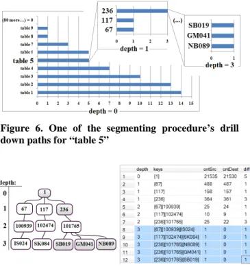
So far, we’ve implemented the CS for the extract/CDC phase. Figure 6 shows the results of one run (for the HEIS DW system [6]). Our procedure found differences in 9 out of 89 tables. Only for “table 5”, figure shows the drill down path that the segmenting procedure takes in discovering smaller and smaller segments containing disparate data. At depth 1, the procedure found three smaller segments (with keys 236, 117 and 67) that were responsible for those five uneven rows at depth 0. Analogously, those three segments were “drilled” to find even smaller segments at depth 4. Note that, for clarity, figure shows only one path (and skips the depth=2 step). Figure 7 shows a complete drill down tree that the segmenting procedure traverses. Nodes traversed in Figure 7 are shown in grey. Figure 7 also shows part of the table that stores the results.
Figure 6. One of the segmenting procedure’s drill down paths for “table 5”
Figure 7. The full drill down tree for “table 5” and the corresponding result table
Values of attributes used to segment the data are enclosed in square brackets, concatenated and stored in a text field named “keys” (since it is required to store various number of arbitrarily typed keys). Other column names are self explanatory. Using metadata, these rows can easily be translated to SQL statements, e.g. the last row in the table in the Figure 7 evaluates to:
WHERE universityId = 236 AND departmentId = 10765 AND personId = ’SB019’.
All the errors found in this run were accredited to date range mismatch between our source system (Informix) and data warehouse system (MS SQL Server 2000) because MS SQL Server (prior to version 2008) cannot store dates prior to year 1753. However, in the past, we’ve also experienced errors due to schema change (e.g. an attribute in the source system was changed to nullable attribute or, for instance, primary key was expanded in the source system) and other technical reasons (e.g. loader account permissions were erroneously changed). The intention is to run this program on every ETL run, immediately after the transfer of the data to the staging area and, if differences are found, alert the staff.
9 CONCLUSION
This paper introduces a generic procedure for integration testing of ETL procedures. ETL procedures
are implicitly tested by comparing datasets at three locations. We have identified three major challenges in this area: (a) to successfully compare datasets in the data warehousing environment it is necessary to link source and destination records, that is, it is necessary to establish
data lineage (b) calculating differences on large data sets
can be very demanding, even not feasible in a reasonable time and resource frames and (c) tests should be reusable and applicable to existing data warehouse systems.
With respect to that we make following contributions: (a) An easy to implement data lineage mechanism that requires negligible interventions in the existing ETL procedures
(b) Segmenting procedure that explores differences in data sets in an OLAP style drill down manner. Procedure is tunable with respect to the depth of the data exploration. Greater depth implies smaller segments, or better precision.
With these two mechanisms we design a generic testing architecture that can be attached to existing systems. We comment on these issues both in terms of incremental load and full reload. Proposed system “grows” with given source(s) and data warehouse systems, collecting valuable information. On incremental loading, this information is leveraged to efficiently find differences only in new (changed) data, whilst maintaining accurate the overall differences state.
In order to achieve this, two assumptions are made (which constitute the limitations of our approach): (i) data warehouse employs dimensional model and (ii) only relational databases are considered as data sources. Future work includes overcoming these limitations and full implementation of proposed procedure in the real world project (as it is now only partially implemented). Furthermore, we plan to formally describe the segmenting procedure algorithm.
In conclusion, proposed procedure pertains only to a few aspects of data quality and by no means provides a comprehensive verification of data warehouse data. It covers counts and basic measure amounts for a subset of data warehouse structures and presents a step towards improving the quality of the data in the data warehouses. It is a fundamental testing strategy that should be augmented with other kinds of test. In such complex systems, one can never be completely certain that data in the data warehouse is an accurate representation of data source(s). It is possible only to be more or less certain. REFERENCES
[1] M. Golfarelli, S. Rizzi:A Comprehensive Approach to Data
Warehouse Testing. Proceedings 12th International Workshop on Data Warehousing and OLAP (DOLAP 2009), Hong Kong, China, 17-24, (2009).
[2] G. J. Myers: The Art of Software Testing (Second Edition), John
[3] Y. Cui, J. Widom, J. L. Wiener: Tracing the lineage of view data in a warehousing environment. ACM Transactions on Database Systems, 25(2):179–227, (2000).
[4] C. Batini, C. Cappiello, C. Francalanci, A. Maurino:
Methodologies for data quality assessment and improvement, ACM Computer Survey, Vol. 41, No. 3, 1-52 (2009)
[5] Y. Wand, R. Wang: Anchoring data quality dimensions in
ontological foundations, Communications of the ACM, Vol 39, Issue 11, 86-95 (1996).
[6] I. Mekterović, Lj. Brkić, M. Baranović: Improving the ETL
process and maintenance of Higher Education Information System Data Warehouse. WSEAS transactions on computers. 8, 10; 1681-1690, (2009).
[7] R.Y. Wang, M. Ziad, Y.W. Lee: Data Quality. Kluwer Academic
Publishers, Norwell, Massachusetts, (2001).
[8] D. Loshin: Enterprise Knowledge Management: The Data Quality
Approach, Morgan-Kaufmann, (2001)
[9] M. Jarke, M. Lenzerini, Y. Vassiliou, P. Vassiliadis: Fundamentals
of data warehouses. Springer, Berlin et al., (2000).
[10] C. Batini, M. Scannapieco: Data Quality: Concepts,
Methodologies and Techniques, Springer-Verlag New York, Inc. Secaucus, NJ, USA, (2006).
[11] T. C. Redman: Data quality: the field guide, Digital Press Newton,
MA, USA, (2001).
[12] L. English: Improving Data Warehouse and Business Information
Quality. Wiley, New York et al. (1999).
[13] C. Thomsen, T. B. Pedersen: ETLDiff: A Semi-automatic
Framework for Regression Test of ETL Software, Lecture Notes in Computer Science, Springer Berlin/Heidelberg, Volume 4081/2006, 1-12, (2006).
[14] T. Friedman, A. Bitterer: Magic Quadrant for Data Quality Tools,
25 June 2010,
http://www.gartner.com/DisplayDocument?id=1390431&ref=g_si telink&ref=g_SiteLink
[15] J. Barateiro, H. Galhardas: A Survey of Data Quality Tools,
Datenbank Spectrum 14, (2005)
[16] J. Rodić, M. Baranović: Generating data quality rules and integration into ETL process., Proceedings 12th International Workshop on Data Warehousing and OLAP (DOLAP 2009), Hong Kong, China, 65-72, (2009).
[17] M. Helfert, C. Herrmann: Proactive data quality management for
data warehouse systems. 4th International Workshop on 'Design and Management of Data Warehouses' (DMDW'), in conjunction with CAiSE, (2002).
[18] M. Helfert, E. von Maur: A Strategy for Managing Data Quality in
Data Warehouse Systems, Sixth International Conference on Information Quality, MIT, Cambridge, USA, (2001).
[19] Y. L. Simmhan, B. Plale, D. Gannon: A Survey of data
Provenance Techniques, ACM SIGMOD Record, September 2005
[20] Y. Cui, J. Widom: Lineage tracing for general data warehouse
transformations, in Proc. VLDB’01, 471–480. Morgan Kaufmann, (2001).
[21] H. Galhardas, D. Florescu, D. Shasha, E. Simon, and C.-A. Saita:
Improving data cleaning quality using a data lineage facility, in Workshop on Design and Management of Data Warehouses (DMDW), Interlaken, Switzerland, (2001).
[22] R. Kimball, M. Ross: The data warehouse toolkit: the complete
guide to dimensional modeling (2nd edition), John Wiley & Sons, Inc; (2002).