Proton pencil beam kernels as extracted from Geant4 Monte Carlo simulations

(1)

Geant4 Monte Carlo simulations

by

Maluba Vernon J. Chisapi

Thesis presented in partial fullment of the requirements for

the degree of Master of Science in the Faculty of

Science at Stellenbosch University

Department of Physics, Stellenbosch University,

Private Bag X1, Matieland 7602, South Africa.

Supervisors:

Prof. Richard T. Newman Mr. Evan A. de Kock

(2)

Declaration

By submitting this thesis electronically, I declare that the entirety of the work con-tained therein is my own, original work, that I am the sole author thereof (save to the extent explicitly otherwise stated), that reproduction and publication thereof by Stellenbosch University will not infringe any third party rights and that I have not previously in its entirety or in part submitted it for obtaining any qualication.

December 2016

Date: . . . .

(3)

Abstract

Proton pencil beam kernels as extracted from Geant4 Monte

Carlo simulations

M. V. J. Chisapi

Department of Physics, Stellenbosch University,

Private Bag X1, Matieland 7602, South Africa.

Thesis: M.Sc. December 2016

The contribution of primary protons, secondary protons, heavy recoil ions, and other secondary particles to the total energy deposited in water by a proton pencil beam (in the therapeutic energy regime) has been investigated using the Geant4 Monte Carlo simulation toolkit. Simulation results have been compared with those calcu-lated using dose distribution functions of the analytical beamlet model of Ulmer et al., which is currently used in the commercial proton treatment-planning package EclipseTM_{. Optimized settings for a robust, accurate, and computationally}

inexpen-sive Geant4 simulations have also been proposed.

(4)

Uittreksel

Proton dun-bundel dieptedosis berekeninge deur middel van

Geant4 Monte Carlo simulasies

(Proton pencil beam kernels as extracted from Geant4 Monte Carlo simulations)

M. V. J. Chisapi

Departement Fisika, Universiteit van Stellenbosch,

Privaatsak X1, Matieland 7602, Suid Afrika.

Tesis: M.Sc. Desember 2016

Monte Carlo simulasies is gedoen met Geant4 om die primêre protone, sekondêre protone, swaar terugslag-ione en ander sekondêre deeltjies se bydraes te bepaal tot die energie wat deur `n dun protonbundel in water gedeponeer word. Hierdie on-dersoek is uitgevoer vir protone in die terapeutiese energiegebied. Die resultate wat vekrei is van die Monte Carlo simulasies is vergelyk met dosisverspreidings wat breken is venaf die analitiese dun-bundel model van Ulmer et al. Dié model word tans gebruik in die EclipseTM _{stelsel, wat `n kommersiële beplanningsisteem vir}

pro-tonterapie is. Verstellings word ook verskaf wat verseker dat die Geant4 simulasies geoptimaliseer is in terme van robuustheid, akkuraatheid en berekeningspoed.

(5)

Acknowledgements

My sincere gratitude to my supervisors: Prof. Richard T. Newman and Evan A. de Kock for giving me the opportunity to study under their supervision, their enlight-ening academic support and guidance. Special thanks to Evan de Kock for charting the direction of this work and his most appreciated input throughout the course of the study. I would also like to thank God for good health and sustenance during my studies. I am indebted to my family for their continued support, and all colleagues and friends for discussions and conversations exchanged.

I am particularly grateful to Alexander Howard of CERN and Jeysingam Jeyasug-iththan of the Department of Clinical Oncology of Jana Teaching Hospital for their assistance on Geant4 related matters.

This thesis would not be possible, had it not been for the nancial and academic support of the following institutions: the African Institute of Mathematical Sciences (AIMS), the Faculty of Science and the Department of Physics of Stellenbosch Uni-versity, the University of Zambia, and the National Research Foundation (NRF) through iThemba LABS.

(6)

Dedications

This thesis is thankfully dedicated to my late loving mother Genevieve Esther Chisapi who inspired me and did everything she could to ensure I get an education,

I will forever love you.

(7)

List of Figures

1.1 Bragg peaks of proton beams . . . 3

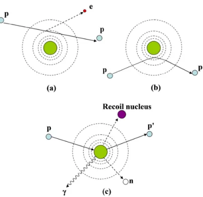
2.1 Proton interaction mechanisms . . . 15

2.2 Multiple Coulomb scattering . . . 16

2.3 Dose contribution of primary protons and the secondaries . . . 22

4.1 The dose distribution for secondary reaction protons . . . 38

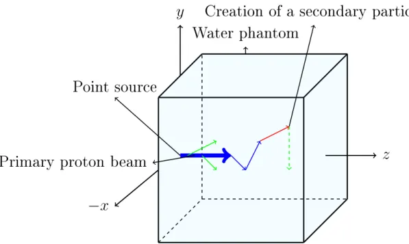
5.1 Illustration of the transport of a proton beam in the water phantom . . . 42

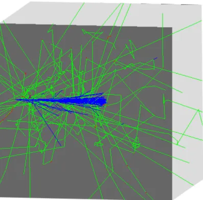
5.2 The transport of proton beam in water . . . 43

5.3 Simulation speed and the eects of the step size on dose distributions . . 47

5.4 Dose deposition geometry. . . 49

6.1 Sensitivity of dose distributions to dierent physics models . . . 52

6.2 Results for 230 MeV incident protons (part 1) . . . 54

6.8 Dose contributions of pp, sp, and rc for 230 MeV . . . 59

D.1 Normalization of radial dose curves . . . 70

D.2 Un-normalized dose distributions. . . 71

E.1 Lack of convergence due to single cut-o value . . . 73

E.2 Convergence as a result of special cut-o values . . . 74

(10)

List of Tables

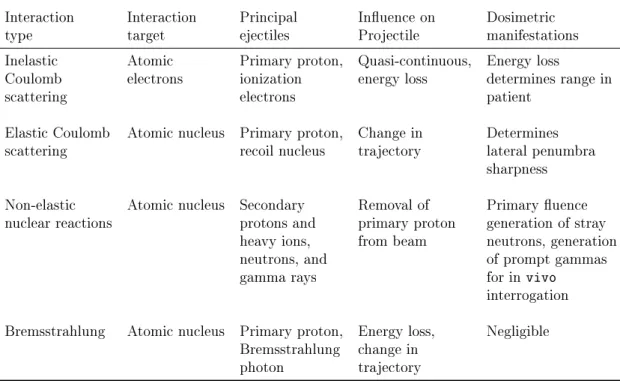
2.1 Summary of proton interaction types . . . 12

4.1 Parameter values for αi and pi (i= 1, ..,4) . . . 32

4.2 Parameter values for ai (i= 1, ..,4) . . . 32

4.3 Parameter values for Ak and βk (k= 1, ..5) . . . 32

4.4 Energy dependent parameters (Ci (i= 1, ..,4)) . . . 34

5.1 Physics models and processes used in Geant4 simulations . . . 45

5.2 Models implemented in the QGSP_BIC_EMY reference physics list. . . 46

5.3 Simulation control parameters . . . 48

5.4 StepF unction parameters . . . 48

6.1 The FWHM, entrance-to-peak dose ratio, and the R80 . . . 58

C.1 Acronyms used to refer to various hadronic options. . . 68

C.2 Suxes used to refer to EM options. . . 68

(11)

Chapter 1 Introduction

Since the rst hospital-based proton therapy center was established in the 1990s, proton radiation therapy has continued to gain popularity in cancer treatment. Hun-dreds of dierent types of cancers (emanating from dierent body tissues) are being diagnosed today. Some of them are not only dicult to cure with prevalent meth-ods (e.g., surgery, chemotherapy, x-ray or radiotherapy), but their treatment with methods such as radiotherapy could lead to exposure of surrounding healthy tis-sue or critical organs to damage by radiation. Conventional photon radiation has been used extensively to treat certain tumours, either alone or in combination with other modalities. Any form of cancer treatment plan involving radiation is adopted based on its ability to deliver suciently high dose to the target volume, with the aim of eradicating the cancerous tumour, while limiting dose falling on healthy tissue as much as possible to avoid late eects and toxicity. With the advent of improved computing, imaging, and scanning technology, photon therapy has under-gone tremendous improvement over the past 15 to 20 years. For example, three-dimensional conformal radiation therapy (3D-CRT), intensity modulated radiation therapy (IMRT), image-guided radiation therapy (IGRT), volumetric modulated arc therapy (VMAT), and intensity modulated arc therapy (IMAT), used today in many cancer treatment centers, are some of the external-beam radiation techniques that are taking advantage of the signicant computer technology evolution currently happening around the world.

However, the energy-loss characteristic of protons traversing matter shows a lot of potential insofar as optimizing trade-os between irradiating the target with a high energy conformal beam and limiting the dose to critical structures is concerned [1]. Several authors writing on this topic have shown that proton therapy has all the exibility of the photon radiation, plus the possibility to control the penetration depth of the proton beam in the target volume [2].

(12)

1.1. A brief historical background of proton therapy 2 In clinical cancer treatment, proton beams within the therapeutic energy regime of about 50-250 MeV, depending on the depth and or size of the tumour volume in the patient, are used. The common approach is to accelerate protons from their source by using particle accelerators (usually synchrotrons or cyclotrons) to dierent treatment rooms. Devices such as bending and focussing/defocussing magnets are placed along the beam line to guide the beam to the treatment rooms. As proton therapy continues to grow, researchers around the world have continued the quest for better and more reliable ways of getting the most out of this modality insofar as increasing the probability of curing the cancer is concerned.

1.1 A brief historical background of proton

therapy

Since the rst medical application of ionizing radiation, in the form of x-rays, was reported in 1895 [3] many technical advancements relating to the manner in which radiation is administered to patients, bearing in mind its eects on biological tissue, have been made. The adaptability of various technologies to the ionizing radia-tion therapy and the notable evoluradia-tion in the computing world has led to radiaradia-tion therapy becoming one of the main treatment options for cancer. The challenge in external-beam radiation method of cancer treatment has always been with how to reduce dose to healthy tissue while increasing or maintaining prescribed dose to tar-get volumes. Techniques such as computerized treatment planning, patient setup, advanced imaging, introduction of intensity-modulated radiotherapy (IMRT), etc., have tremendously transformed the way ionizing radiation is delivered to target vol-umes in the history of radiation therapy. In addition, dose deposition characteristics of dierent type of particles can also go a long way in improving beam delivery ac-curacy [1]. In fact, the medical use of proton beams (and other heavy ions) was rst proposed in 1946 by R. H. Wilson [4] primarily because of the physical characteristics of the way they interact with matter. Wilson observed that the well known physics of proton interactions and their energy loss in matter had the potential to enhance delivery of higher radiation doses to the target volumes relative to `conventional' photon radiation therapy. Protons lose their energy mainly through electromag-netic (EM) interactions with orbital electrons of atoms of the target medium. As the protons slow down, energy transfer to tissue per unit length increases. This leads to almost uniform energy loss over a certain penetration depth (dependent on incident proton energy) but increases sharply to the maximum before a subsequent sharp distal fall o as protons come to a stop (near the end of the range), resulting

(13)

1.1. A brief historical background of proton therapy 3 in a depth-dose peak commonly referred to as the Bragg peak, Fig. 1.1, (after W. H. Bragg) [5].

Figure 1.1: A sharp Bragg peak due to near-monoenergetic proton beams, a SOBP re-sulting from weighted summation of Bragg peaks of dierent ranges, and Bragg peaks with varying ranges. Image sourced from [6].

A near-monoenergetic proton beam exhibits a very narrow Bragg peak, Fig. 1.1. In order to get a Bragg peak that extends longitudinally in width and spreads over the target volume (also known as spread-out Bragg peak (SOBP)), beams of dierent ranges and weights are added together. Variations in proton beam range can be realized by employing various techniques, such as altering the machine energy or placing an adjustable-degrader, e.g., a double wedge, across the beam line. Wilson also suggested utilizing the Bragg peak and the nite range of proton beams for treating tumours seated deep within healthy tissue or close to critical organs [4]. A couple of years after Wilson rst proposed the use of protons (and heavy ions) for cancer treatment, some individuals and institutions began to explore the idea further, rst by trying to get an insight on the biological eects of proton radiation. For instance, Lawrence et al. at Lawrence Berkeley Laboratory (LBL) published their work on the biological study of protons on mice in 1952 [7]. Similarly, in 1955 radiation oncologists at Gustav Werner Institute in Uppsala, Sweden, ran experi-ments on a series of animals (rabbits and goats) [8] [9] to study the biological eect of proton radiation, while at Harvard Cyclotron Laboratory (HCL), extensive relative

(14)

1.1. A brief historical background of proton therapy 4 biological eectiveness (RBE) [10] [11] studies of protons were done in the 1960s. Initially, the major emphasis for proton therapy clinical research was on dose es-calation for tumors which had poor local control with conventional radiotherapy [2].

By the early 1990s, proton therapy was still at the experimental stage, based mainly in research institutions [1]. More work still needed to be done to attain a full-scale use of this treatment modality. For example, many proton machines had limited beam energy, hence could not treat deep seated tumours. They also had xed horizontal beam lines and limited choice of beam angles, thus patients had to be immobilized and positions reproduced in every treatment session. Early proton therapy facilities employed a passive beam scattering technique, in which beam modifying devices such as rotating range-modulator wheel, optional range-shifter plates, adjustable energy-degrader, scattering lters, range-compensators, were used to, mechanically, obtain a spread-out-Bragg-peak (SOBP) that conform to the target volume. With the evolution in the computer technology and the availability of devices such as the multi-leaf collimator, the passive scattering has transformed into a more automated beam delivery method. For example, beam shaping is now done with computer controlled dynamic multi-leaf collimators [2].

The technological advancements happening around the world coupled with the in-volvement of commercial companies have given rise to sophisticated equipment as-sociated with proton treatment delivery. Among them are isocentric gantries, which are capable of irradiating a target volume from any arbitrary direction around the pa-tient, accurate imaging equipment such as the PET/CT, which combines a positron emission tomography (PET) scan and a computed tomography (CT) scan, and com-puterized treatment planning programs. This has made possible the adoption of dy-namic proton beam delivery techniques such as spot or pencil beam scanning (also known as the intensity-modulated proton therapy (IMPT)). Compared to passive beam scattering, which uses beam modifying devices to produce a required dose distribution in the target volume, IMPT uses magnets to direct an unmodulated pencil beam from the accelerator (synchrotron) onto the target cross section area (in spot or continuous form) while varying the energy and the intensity to control its penetration depth. IMPT therefore oers proton dose distributions that are highly conformal to the target volume, thereby increasing sparing of the normal tissue. Furthermore, a number of companies around the world today manufacture proton therapy related equipment, making the treatment modality more accessi-ble to the public. The rst hospital-based proton therapy facility, equipped with modern technology, e.g., gantries, was opened in October, 1990 at the Loma Linda

(15)

1.2. Proton dose calculation algorithms 5 University Medical Center (LLUMC) [1]. A few years down the line, more proton therapy centers started mushrooming across the world and the numbers have since been growing steadily [12]. Among the earliest centers to be opened is the iThemba Laboratory for Accelerator-Based Sciences proton therapy facility, which was com-missioned in September 1993 in Cape Town, South Africa. It provides a proton beam with maximum energy of 200 MeV which is used for both medical applications and for research purposes [13]. Currently, there are over sixty operational proton ther-apy centers around the world and over thirty more are scheduled for commissioning within the next two to three years [14].

1.2 Proton dose calculation algorithms

The wide acceptance proton therapy is currently receiving across the globe has heightened the need for accurate and relatively fast dose calculation algorithms. For routine clinical treatment planning, analytical dose calculation algorithms are preferred as they are both feasible and computationally fast compared to Monte Carlo [15] methods. Several forms of proton dose calculation algorithms exist today, the majority of which are based on the pencil beam model [16] [17] [18].

The pencil beam model is a mathematical model attempting to zoom in and assim-ilate the dose-deposition process of a very narrow (and near-monoenergetic) proton beam in the patient and subsequently approximating the eect of such interaction processes for a broad beam. The pencil beam model, based on the Fermi-Eyges the-ory of particle transport [19], was rst applied to electron dose calculation algorithms by Hogstrom [16]. With suitable modications however, his formalisms are widely used today in proton pencil beam dose calculation algorithms. Hogstrom denes a pencil beam as a narrow particle beam with innitesimally small lateral dimension (cross section) impinging at a point on a semi-innite medium [16]. The dose de-livered by the broad beam is approximately equal to the sum of dose deposited by individual near mono-energetic pencil beams. In other words, this approach sug-gests that a 3D broad beam is made up of an innitely large number of narrow pencil beams impinging on the surface of the medium [20]. Due to inhomogeneity of the medium, these pencil beams lose their energy dierently even though they are subject to similar interaction processes. Several authors have shown that individual pencil beam dose distributions can indeed be summed up to give, approximately, the total dose deposited in the medium by the broad beam [21] [16] [17] [22]. A good proton-dose calculation algorithm must take into account all possible energy loss processes while being both accurate and relatively fast. To date, a number of

(16)

1.3. Monte Carlo simulations 6 algorithms used to predict proton-dose distribution in the patient have been devel-oped using dierent approaches [17] [18] [23] [22] [21] [24] [25]. While the majority of these dose-calculation algorithms have to some extent compromised accuracy for the sake of achieving clinically viable computational speeds, a few of them, e.g., Ulmer's beamlet model, have attempted to take into account all the physics while remaining computationally inexpensive. The rate of energy loss per unit track length (stopping power) in dierent material have been successfully calculated using the Bethe-Bloch equation (BBE) and the results [26] [27] are widely used to develop relatively fast dose-calculation algorithms. On the other hand, incorporating an algorithm that gives a comprehensive description of multiple Coulomb scattering (MSC) can be quite involved. Various MSC theories e.g., Molière's [28] (known to be the most comprehensive), Highland's [29], Goudsmith and Saunderson's [30], Lewis' [31], etc., exist today. The choice of the MSC theory for a proton dose-calculation algorithm to be used in a treatment planning system (TPS) can depend on the feasibility to incorporate it and/or the trade-os between the accuracy and the computational speed. Usually, relatively less involved theories, such as Highland's, are employed or minor permissible modications are made to the original MSC theory in order to achieve a clinically viable analytical dose-calculation algorithm. Literature shows that, with a few exceptions, a large number of proton pencil-beam algorithms in use today either improve on or are a generalization of the Fermi-Eyges theory [16] [32] [33] [34], which is a relatively simple particle-transport theory [19].

1.3 Monte Carlo simulations

Modern approaches to deriving proton-dose calculation algorithms try to use data from Monte Carlo (MC) simulations [25] [35] as these (MC methods) account for all physical processes, thereby providing the most accurate means of approximating proton energy-deposition in matter and the interaction of radiation with matter in general [1] [36]. Besides providing a practical alternative to measured beam proles, MC methods are capable of simulating scenarios that may prove dicult or impossible to do experimentally [1]. These can also save beam time by reducing the need for experiments. Basically, MC simulations can be used for predicting dose distributions in the patient, studying the physics of proton beams, designing and testing the beam delivery system, for quality assurance purposes, and so on [1] [37]. In general, a MC method (or simulation) is a numerical method for approximating the probability of a certain outcome by using randomly sampled numbers from a probability density function. MC methods are mainly used to nd numerical

(17)

solu-1.3. Monte Carlo simulations 7 tions to problems that are too complicated to solve analytically. Random number generators used in modern day computers have very long periods, making them capable of simulating complex stochastic processes before the sampled number se-quence eventually repeats itself. Conceptually, a MC algorithm takes as input the numbers sampled randomly from a probability distribution and performs a calcu-lation. In radiotherapy, the probability distribution could represent possible ways a particle might interact in a given step consistent with the laws of physics. The calculation is performed repeatedly over a very large number (N) of samples, thus, allowing the simulation of all possible outcomes. The result is a probability distri-bution of a certain outcome, which converges as N → ∞. The uncertainty in the

result decreases with increasing number of samples taken, N (i.e., ≈1/√N).

Charged particle transport in matter depends on the interaction probabilities (i.e., cross sections) per unit distance [36]. MC methods are widely used today in radiation therapy to simulate physics interactions on a step-by-step basis. At each step of the particle's passage through the medium, the probability of physics interactions and their outcomes is represented by probability density functions, making the simulation equivalent to solving the Boltzmann particle-transport equation for protons [1].

1.3.1 Geant4 Monte Carlo detector simulation toolkit

Geant4 (i.e., GEometry AND Tracking) is an open source Monte Carlo detector sim-ulation toolkit for simulating passage of particles (radiation) through matter [38]. It is developed and maintained by an international collaboration of physicists and soft-ware engineers (Geant4 collaboration) from all around the world [39]. The Geant4 code is written in object-oriented C++ programming language and is widely used

in high energy physics, space science, nuclear and accelerator physics as well as in medical sciences. Besides oering versatile ways of tracking particles in the medium with realistic magnetic or electric elds, the Geant4 detector simulating toolkit com-prises a comprehensive collection of a large variety of particles, physics processes, models and cross-section libraries for particle transport in matter. Because of its complexity, the Geant4 code relies signicantly on the optimized computing power of modern computers (e.g., multi-threading) and the extensible nature of object-oriented C++. Moreover, the Geant4 kernel (central unit) is designed to work in

conjunction with non-Geant4 graphic systems and interfaces, such as OpenGL, Qt, DAWN, and ROOT, to aid visualization of the geometry and trajectories as well as for data analysis purposes [40] [39] [41]. The Geant4 toolkit therefore allows for development of a program capable of carrying out tasks from the initial problem denition all the way through to the generation of results, or even nal plots for

(18)

1.4. Objectives and aims 8 publication [38].

1.4 Objectives and aims

The main aim of this work is to generate pencil beam kernels (i.e., 3D dose distribu-tions in water) by simulating the traversal of proton pencil beams in the energy range of clinical interest (i.e., 50-250 MeV) through water using the Geant4 MC simulation toolkit, and to assess the contribution of primary protons, secondary protons, and heavy recoil ions and other secondary particles to the total absorbed dose. Such investigations will lay a foundation for future development of an in-house MC-based analytical model for pencil-beam kernels (and eventually a pencil-beam dose cal-culation algorithm) for the iThemba LABS proton therapy program. This work is motivated by the analytical proton beamlet model of Ulmer et al. [35], which is par-tially implemented in the commercial proton treatment planning system, EclipseTM_,

of Varian medical systems1_{. The beamlet model will therefore be used mostly as}

a reference point. Like in the beamlet model, the energy deposited in water will be sorted into the following categories: primary protons (pp), secondary protons (sp), and a third group comprising heavy recoil ions and other secondaries which will be denoted as (rc). Both the radial and depth-dependent components of the energy deposited by each particle category will be investigated at respective depths and for the longitudinal depth, respectively. To embark on this undertaking, it was necessary to rst learn the formalism of the Geant4 detector simulation toolkit and establish an optimized list of the simulation control parameters and physics settings for a robust, fast and accurate MC (Geant4) simulations.

1.5 Thesis structure overview

Chapter 2 discusses the dierent ways in which proton beams interact with matter. It describes the basic physics of proton energy loss and the production of secondary particles. This chapter ends with a brief explanation of how these interaction pro-cesses are included in the Geant4 simulation toolkit.

Chapter 3 covers the mathematical denitions of simple proton beam congurations. It also introduces the mathematical description of dose deposited (the pencil beam kernel) at a given point in the medium by a very narrow proton beam (pencil beam). The rest of the chapter discusses ways dierent types of particles contribute to the 3D dose deposition by a pencil beam.

(19)

1.5. Thesis structure overview 9 In chapter 4 the derivation of the analytical proton beamlet model by Ulmer et al. is outlined.

Chapter 5 covers the simulation of the passage of proton pencil beams (of clinical energy range) through water using the Geant4 (MC) toolkit. An optimized simula-tion parameter list is suggested, the physics models are discussed, and the general setup and settings for the Geant4 simulations are outlined.

Chapter 6 discusses the results from the simulations. A comparison of dose distri-butions from the Geant4 simulations and the Ulmer beamlet model are also given here.

A conclusion is presented in chapter 7 together with an outline on possible future work.

(20)

Chapter 2 Proton interaction mechanisms

The interaction of protons with matter takes place via three distinct processes: they suer energy loss by electromagnetic (EM) collisions with atomic electrons, multiple Coulomb deections by atomic nuclei, and sometimes undergo nuclear collisions, in which incident protons inelastically scatter o the medium nucleus, leaving it in the excited state, or physically knock constituent protons, neutrons, or light nucleon clusters out of the nucleus [1]. In this chapter we review the physics of proton interactions with matter.

2.1 Energy loss processes

Protons traversing a given target medium (e.g., water) lose energy mainly through electromagnetic (EM) collisions with atomic electrons, causing them to eventually stop in the medium. Although important only at incident energies far less than the clinical range (below 20 keV [26]), protons also lose energy by elastic EM collisions with atomic nuclei, giving rise to the so-called nuclear stopping power Snuc [42].

A proton (or a charged particle) penetrating the medium interacts with the atoms via the Coulomb force, leading to excitation of the atomic electrons or ionization of the atoms (see Table 2.1). This is the main process by which protons traversing matter lose their energy. Apart from that, incident protons can physically eject orbital electrons from the atom (see Table 2.1 and Fig. 2.1(a)). Ejected electrons are calledδ-rays and have kinetic energy equivalent to that lost by projectile protons.

As protons slow down in the medium, the rate of energy loss increases, leading to a sharp increase in ionization of the medium atoms near the end of the range, thus leading to the Bragg peak. According to Gottschalk, the range R0 of a

quasi-monoenergetic proton beam is dened as the depth of material at which half the

(21)

2.1. Energy loss processes 11 protons that undergo only EM interactions have stopped [1] [42]. For water, this range can be approximated as

R0 ≈d80, (2.1.1)

where d80 is the depth in water corresponding to the distal 80% point of the Bragg

peak [42] [1]. An incident mono-energetic proton beam may be assumed to be un-dergoing continuous interactions (hence losing energy continuously) as it penetrates a homogeneous medium. Such an approximation allows for uctuations in energy loss to be ignored, therefore, the so-called continuous-slowing-down-approximations (CSDA) [35] technique can be used to approximate the range RCSDA of the proton

beam in the medium. In the CSDA framework, protons in the incident mono-energetic beam would be assumed to eventually stop at the same depth in the medium. However, whether their initial energy is the same or varies, protons travers-ing matter have been observed to stop at dierent points (even if the medium is homogeneous), a phenomenon referred to as energy or range straggling1 _{[26]. Janni}

[26] explored the theory of straggling and showed that range straggling in light (low Z) and heavy (high Z) materials dier only slightly, meaning that the shape of the Bragg peak almost remains the same when, say, water is replaced by plastic or lead (Pb). Changing the incident proton energy however changes both the peak-to-plateau ratio of the Bragg curve and its shape [25].

2.1.1 The stopping power

The amount of energy lost per unit distance travelled by a charged particle through the medium, also known as the linear stopping power S ≡ −dE/dz (MeV/cm), is a

function of the incident particle energy and the target material [1]. In proton therapy however, the mass stopping power S/ρ≡ −dE/ρdz (MeV/(g/cm2_{)), dened as the}

amount of energy lost per unit areal distance, is frequently used. The mass stopping power equation was derived around 1933 by Bethe and Bloch [26]. For an elemental target with atomic number Z and relative atomic mass A, traversed by a projectile of charge zeand velocity v =βc, S/ρ can be calculated by

−1 ρ dE dz = 4πr2 emec2 β2 1 u Z Az 2_L₍_β₎_. _(2.1.2)

The quantity L(β) is called the stopping number. It accounts for the ne details of

the energy loss process. The factor 4πr_e2mec2/u is a material-independent constant

1_{Energy straggling as a result of uctuations in energy loss, or range straggling to refer directly}

(22)

2.1. Energy loss processes 12

Interaction Interaction Principal Inuence on Dosimetric type target ejectiles Projectile manifestations Inelastic Atomic Primary proton, Quasi-continuous, Energy loss

Coulomb electrons ionization energy loss determines range in scattering electrons patient

Elastic Coulomb Atomic nucleus Primary proton, Change in Determines scattering recoil nucleus trajectory lateral penumbra

sharpness Non-elastic Atomic nucleus Secondary Removal of Primary uence nuclear reactions protons and primary proton generation of stray

heavy ions, from beam neutrons, generation neutrons, and of prompt gammas gamma rays for in vivo

interrogation Bremsstrahlung Atomic nucleus Primary proton, Energy loss, Negligible

Bremsstrahlung change in photon trajectory

Table 2.1: Summary of proton interaction types, targets, ejectiles, inuence on projectiles, and selected dosimetric manifestations, Table by [43].

approximately equal to 0.307075 MeV cm2 _g−1_{. The constant} _r

e is the classical electron radius = 2.817×10−13 _cm, _u _{is the atomic mass unit, and} _m

ec2 ≈ 0.511 MeV is the electron rest energy. The quantity L can be written as

L(β) = L0(β) +zL1(β) +z2L2(β), (2.1.3)

where zL1 is the Barkas correction, and z2L2, the Bloch correction. Bethe derived

the stopping power theory on the basis of the rst-order Born approximation. These corrections account for departures from this approximation, and are important only at low projectile velocities (i.e., lower than velocities of the atomic electrons) [44]. The term L0 is given by

L0(β) = 1 2ln 2mec2β2Wm (1−β2₎_I2 −β2− C Z − δ 2, (2.1.4)

where C/Z is the target shell correction, and δ/2, the relativistic density-eect

cor-rection, I is the mean excitation energy of the target material (discussed in Sec. 2.1.1.1). The factor Wm is the maximum energy that can be transferred to an unbound electron at rest in a single proton-electron collision [1]. It is given by

Wm = 2mec2β2 1−β2 × 1 + 2me mp(1−β2)1/2 +me mp −1 . (2.1.5)

The factor in the square brackets is nearly unity and contributes only at relativistic energies. For clinical incident energy range, Eq. (2.1.8) is a reasonably accurate

(23)

2.1. Energy loss processes 13 approximation for the full relativistic description.

The density-eect δ and the shell correction C are important only at high and low

energies respectively [45]. The density-eect δ arises from the fact that a proton

polarizes the atoms along its path, leading to the disturbance in the electron eld which in turn reduces the inuence of the outer lying electrons on the proton energy loss [26] [45]. The density-eect becomes more important at incident energies far beyond the clinical energy regime and for high medium densities. On the other hand, the shell correction accounts for eects arising when the incident particle velocity becomes less or equal to the orbital velocity of the bound electrons. At such energies, the assumption that the electron is at rest relative to the incident particle is no longer valid and the Bethe-Bloch formula without the shell correction term breaks down [45].

2.1.1.1 The mean excitation potential

The mean excitation energy (or ionization potential) I of the target material is a material dependent quantity and by far the main source of uncertainty in the clinical energy range [1]. In practice, it is very dicult to calculate I with sucient accuracy. Therefore, it is usually obtained by tting measured range-energy values (for materials where data exists) or interpolated with the guidance of the theory [42] (in cases where measurements are unavailable). For media of unknown ionization potential, Bragg's additivity rule:

S ρ = X i wi S ρ i , (2.1.6)

is used. Here, the term wi is the fraction by weight of the ith element. Bragg's additivity rule suggests that mass stopping power for mixtures or compounds can be estimated by the linear combination of the stopping powers of the constituent elements [46]. However, because of the signicant inuence the chemical bonding in compounds has on the mass stopping power Eq. (2.1.6) is largely an approximation. Range-energy tables can slightly dier depending on the author's choice for the I value. In Geant4, I values recommended by ICRU [44] are used [47].

Overall, the Bethe-Bloch formula is accurate enough for the radiotherapy energy regime and it is permissible to omit most of these corrections [1] in this energy range. Eq. (2.1.2) can therefore be used in its simplest or non-relativistic form:

S ρ ≡ − 1 ρ dE dz = 0.307075 Z A 1 β2 lnWm I −β 2 M eV g/cm2, (2.1.7) with Wm = 2mec2β2 1−β2 . (2.1.8)

(24)

2.2. Multiple Coulomb scattering 14 At very low energies (e.g., / 2 MeV), this formula is no longer accurate, therefore,

the corrections must be implemented. Implementing these corrections can be quite involved mathematically, especially in the already complicated MC codes. Several authors [46] [26] [44] have calculated the mass stopping powers of various material for clinical incident proton energy range which are today tabulated into range-energy tables, e.g., of Janni [26], ICRU report 49 [27], etc. These look-up tables are used in most MC codes today, which would otherwise take very long to execute.

In the Geant4 toolkit, the Bethe-Bloch equation is used to calculate the hadron energy loss down to 2 MeV, below which a parameterization based on the ICRU report 49 [44] is implemented [48]. In Geant4, any interaction process calculates the continuous and discrete energy loss in the medium. Above a given energy threshold (range cut) the energy loss of the particle is simulated by the explicit production of secondary particles (gammas, electrons, positrons, protons, etc.) while below the threshold, the energy loss is treated as continuous [47]. Therefore, if a given particle suers continuous energy loss via several processes, the total continuous part of the energy loss will be the sum. In order to speed up the simulations, the continuous energy loss (which occurs at very low energies depending on the user-dened cut-o value) is pre-calculated during the initializaticut-on phase cut-of the Geant4 simulaticut-on and stored in the dE/dz table. The ranges of the particle in a given material are then calculated using this table and stored in the Range table, which eventually is inverted into the InverseRange table. At run time, values of the continuous energy loss and range are obtained using these tables. Discrete energy loss is not involved at this stage. In contrast to the continuous energy loss, the production of secondary particles above the production threshold is sampled explicitly by each energy loss process [47].

2.2 Multiple Coulomb scattering

Protons passing through matter may also get deected by atomic nuclei, a process commonly referred to as scattering, more precisely, multiple Coulomb scattering since the observed angular dispersion is due to a cumulative eect of many random small single-scatterings. Both the proton and the nucleus have a positive charge, as such, their interactions are largely electrostatic in nature (as a result of the Coulomb force acting between them, see (b) in Figure 2.1). Such large numbers of small single-deections are better treated statistically. The overall spatial distribution tends towards a Gaussian (Figs. 2.2a and 2.2b) provided the scattering events occur at small angles, a condition largely satised by protons traversing a low Z medium such

(25)

2.2. Multiple Coulomb scattering 15

Figure 2.1: Schematic illustration of proton interaction mechanisms: (a) energy loss via inelastic Coulomb interactions, (b) deection of proton trajectory by repulsive Coulomb elastic scattering with nucleus, (c) removal of primary proton and creation of secondary particles via non-elastic nuclear interaction (p: proton,e: electron, n: neutron, γ: gamma rays). Image from Newhauser [43].

as water or plastic [1].

Several theories of multiple scattering have been developed since the 1930s [28] [1]. In the Gaussian approximations the main focus is the dependence of the mean scattering angle θ0 on proton energy and scattering material as well as its thickness.

The so-called Molière's characteristic multiple scattering angle θM, given by

θM = 1 √ 2(χc √ B) (2.2.1)

is analogous to θ0 [1]. In Eq. 2.2.1, χc is the characteristic single scattering angle. For an incident proton (charge number z, momentum p, speed v) passing through

a signicantly thin target (t:thicknessproton range) consisting of a single element

(atomic weight A, atomic number Z), χc can be written as

χ2_c =c3t/(pv)2, (2.2.2) where c3 ≡4πNA e2 ~c 2 (_~c)2z 2_Z2 A , (2.2.3)

and B is the reduced target thickness,

(26)

2.2. Multiple Coulomb scattering 16

(a) MCS in thin slab.MP-Measuring

plate. (b) Lateral scattering due to MCSyields a Gaussian.

Figure 2.2: Multiple Coulomb scattering resulting from proton interactions with nuclei of medium atoms (images from [1] and [49] respectively).

NA ≈6.022×1023 mol−1 is Avogadro's number, e2/~c≈1/137 is the ne structure constant, and ~c ≈ 197× 10−13 MeV cm is the conversion factor. The quantity

b is the natural logarithm of the eective number of collisions in the target. The physical interpretation of χc is that, on average, a proton suers exactly one single scatter greater than χc in its traversal of the target [1].

Dening a reduced angle,

θ0 ≡ θ

χc

√

B (2.2.5)

Molière approximates the angular distribution function f(θ) of the proton space

angle θ by a power series in 1/B: f(θ) = 1 2πθ2 M 1 2 f(0)(θ0) + f (1)₍_θ0₎ B + f(2)₍_θ0₎ B2 (2.2.6) where the f(n) _{are given by}

f(n)(θ0) = 1 n! Z ∞ 0 ydyJ0(θ 0 y)ey1/4 y2 4 ln y2 4 n . (2.2.7) and f(0) is a Gaussian: f(0)(θ0) = 2e−θ 0₂ . (2.2.8)

A good summary of Molière's theory is given in [1], while the detailed theory is in the original papers [28]. Although given here in brief, it can be clearly seen that Molière's theory is mathematically complicated.

(27)

2.2. Multiple Coulomb scattering 17 In subsequent years continuous improvements or re-evaluation of some of these scat-tering theories has been on the rise, with the view of arriving at accurate but easier to evaluate formulae for purposes of clinical dose calculation algorithms. Examples of such undertakings include Highland's formula [29], which he derived by parame-terizing the full Molière/Bethe/Hanson theory, and Urbàn model [50], which is based on the Lewis theory of multiple Coulomb scattering [31].

Highland's formula calculates the mean scattering angle θ0 as θ0 = 14.1MeV pv r L LR 1 + 1 9log10 L LR rad, (2.2.9)

where pv is the kinematic factor given by Eq. (A.0.6), L is the target thickness,

and LRis the radiation length of the target material [1]. The radiation length is the distance over which the incident particle's energy is reduced by a factor e−1(≈0.37)

due to radiation losses alone [51]. This scattering angle is integrated along the beam axis (z-axis), and the lateral standard deviation at depth z (for beam axis coinciding with the z-axis) can be given by

σ_x,2_MCS(Z) = 1 +1 9log10 z LR 2 × Z z 0 14.1MeV pv ×(z−z 0 ) 2 1 LR dz0 . (2.2.10)

Another theory very appropriate for describing the spatial and angular distributions of protons traversing matter is the Fermi-Eyges theory [19]. The Fermi-Eyges the-ory is a relatively simple thethe-ory that describes the propagation of a particle beam through matter. It gives the solution to the Fermi equation which in turn derives from the more fundamental linear Boltzmann equation in two steps [52]: First, with the assumption that the scattering of interacting particles occur over small angles, the Boltzmann equation is approximated by the Fokker-Planck equation. Second, the Fokker-Planck equation is reduced to the Fermi equation by assuming continu-ous energy loss of the penetrating particle (CSDA), that is, the energy of incident particle is a well dened and continuous function of the penetration depth [52] [33]. Ideally, the angular distribution of protons in a given medium approximates a Gaus-sian for small angles (see Figs. 2.2a and 2.2b) followed by a scattering tail, which is eectively governed by the small-angle Rutherford scattering, with dσ/dΩ≈ 1/θ4.

The Fermi-Eyges theory was initially applied to pencil beam algorithms for electron beams by Hogstrom [16].

The Fermi-Eyges theory approximates the lateral spread of an initially parallel and innitesimally narrow proton beam as a function of depth in water, z (in centime-ters), to a Gaussian of width

x2

MCS(z) = σ2x,MCS = Z z

0

(28)

2.2. Multiple Coulomb scattering 18 where the lateral variance of the beam,

x2 MCS(z) = N X i=1 x2_i/N (2.2.12)

is equal to the square of the standard deviation of the Gaussian prole (σ2

x,MCS(z)), in the limit of many scattering events (N), and

T(z)≡dθ2_/dz (2.2.13)

is the scattering power [1], simply dened as the rate of increase of the variance of the MCS angle [53]. However, the commonly used formula for the scattering power is the parameterization,

T(z) = Tdm = [0.524 + 0.1975 log10(1−(pv/p1v1)2) + 0.2320 log10(pv/MeV)

−0.0098 log₁₀(pv/MeV) log₁₀(1−(pv/p1v1)2)]×

Es pv 2 1 LR, (2.2.14) which is called the improved non-local formula, as given by Gottschalk [53]. Here,

pv[MeV] is the product of the proton momentum and velocity and is a function of z; p1v1 is the initial product of momentum and velocity,Es = 15.0 MeV, andLR is the radiation length (36.1 cm for water) [1].

In the Gaussian approximation, each pencil beam evolves in water according to

σx,MCS(z) such that at any depth z the total distribution can be explained in terms of the convolution of two Gaussian functions: the initial unperturbed Gaussian shape and the additional spreading due to MSC in the medium [1].

2.2.1 Multiple Coulomb scattering in Geant4

In order to optimize speed in MC simulations, condensed algorithms are used instead of the detailed algorithms. Detailed simulation algorithms account for every colli-sion/interaction that a simulated particle experiences. A simulation by a detailed algorithm can be considered exact, i.e., it gives the same results as the solution of the transport equation [50]. Because the detailed algorithm simulates every interaction, it can only be used for simulations which involve a small number of collisions, such as the interaction of low energy projectiles with thin foils, or low density gas [50]. On the other hand, condensed simulation algorithms simulate global eects (such as the net energy loss, displacement and change of direction of the charged particle) of the collisions at the end of the step (or track segment). Condensed simulation algorithms are used to simulate high energy particle transport in solid or liquid media where the average number of collisions is very large such that the detailed

(29)

2.2. Multiple Coulomb scattering 19 simulation becomes inecient [50]. The displacement and the change of direction of the penetrating particle are calculated by MSC algorithms that are incorporated in the transport codes. The accuracy of these algorithms is limited by the accuracy of the approximations used in MSC models.

The MSC model used by default in the Geant4 toolkit (since version 10.0) is the G4UrbanMscModel, developed by L. Urbàn [50]. The Urbàn MSC model belongs to the class of condensed simulation algorithms and is applicable to all types of particles at any energy. It is based on the Lewis model of MSC [31], i.e., it uses model functions that have been chosen in such a way as to give the same moments of angular and spatial distributions after a step as the Lewis model [50]. Compared to the Lewis model, the MSC theories of Molière, Goudsmit-Saunderson [30], etc., only determine the angular distribution after a step, they do not compute the moments of the spatial distributions. The G4UrbanMscModel simulates the scattering of the charged particle after a given step, computes the path length correction and the lateral displacement of the particle penetrating the medium [50]. Below (Sec. 2.2.2) we briey discuss the Lewis theory and give a short overview of the Urbàn model.

2.2.2 The Urbàn model of multiple Coulomb scattering

The Lewis theory describes a direct method of obtaining exact results from the dif-fusion equation of the multiple scattering of charged particles traversing an innite and homogeneous medium, without the usual small-angle approximation. In the development of the theory, Lewis carried out an expansion of the cross-section for scattering in spherical harmonics, leading to a diusion equation that rapidly con-verges in the case of large-angle scattering when integrated over all space, and whose coecients can be exactly determined. The determination of the coecients leads to expressions for various moments of spatial and angular distributions. Lewis also showed that his angular distribution result can be transitioned to cases in which only the small-angle scattering is important [31].

Based on the Lewis theory of multiple scattering, Urbàn developed a model for MSC to be used in the Geant4 toolkit. The model uses the transport mean free paths, λi, to determine properties of the MSC process. The i-th transport mean free path is

given by 1 λi = 2πna Z 1 −1 [1−Pi(cosχ)] dσ(χ) dΩ d(cosχ), (2.2.15)

where dσ(χ)/dΩ is the dierential cross section for scattering, Pi(cosχ) is the i-th Legendre polynomial, and na is the number of atoms per volume. Instead of using the cross section directly, the model uses the rst and second transport mean free

(30)

2.2. Multiple Coulomb scattering 20 paths (λ1 and λ2) to compute the dierent spatial and angular distributions. The

straight distance between the endpoints of a step is called the geometrical path length

`, while the total length travelled by a particle is referred to as the true path length t. In order to accurately describe the transport of a particle in matter, the step

limitation imposed by the physics processes and the geometry of the detector are compared and the minimum step length is selected as the actual step length. The role of the MSC algorithm in this capacity is to transform the minimum `physics step length' into `geometrical step length' (i.e., t → `, also known as the inverse

of the path length correction). Once the actual step length is determined and the particle position has changed, the MSC carries out the path length correction: the transformation` →t, since the energy loss and scattering computation need the true

step length t. For instance, at the end of this step length (t) the scattering angle θ

of the particle is sampled according to the model function, and lateral displacement is calculated using the equation (for a particle with the initial direction parallel to the z-axis) hx2+y2i= 4λ 2 1 3 τ −κ+ 1 κ + κ κ−1e −τ ₋ 1 κ(κ−1)e −κτ , (2.2.16)

where τ =t/λ1 and κ=λ1/λ2. The lateral correlation given by

hxυx+yυyi= 2λ1 3 1− κ κ−1e −τ + 1 κ−1e −κτ (2.2.17) determines the direction of the lateral displacement. In Eq. (2.2.17) υx and υy are the xand y components, respectively, of the direction unit vector [50].

Step limitation algorithms are also implemented in the transport process of this model to keep the particle from crossing the volume in one step or to restrict the step size of the particle entering a new volume for the sake of good simulation of backscattering. Similarly, boundary crossing is treated by a stepping algorithm which prevents the last step of the particle from being bigger than the mean free path of elastic scattering in the given volume. This restricts the particle to single scattering at or very close to the boundary [50].

The reliability of the Geant4 MC simulations under the implementation of the Urbàn MSC model has been tested against experimental and Geant32 _{simulation results,}

which implemented Molière's theory [54] [55]. Some benchmarking comparisons have been done for the scattering angle distribution, energy deposit distribution in detec-tors, transmission of charged particles, backscattering of charged particles, etc., in

(31)

2.3. Nuclear interactions 21 dierent media. Overall, with the implementation of the Urbàn MSC model, Geant4 simulation results agree with experimental data within experimental uncertainties. Molière's theory is well known for reproducing the Gaussian type of angular dis-tribution at small angles and the Rutherford-like scattering at large angles. The Lewis theory equally gives a good description of the long single-scattering tail in addition to Gaussian distribution for small-angle scattering. There is yet to be an authoritative comparison of the two theories, as such we cannot categorically state which theory is more accurate. However, the outstanding dierence is that one the-ory (Molière's) calculates only the angular distribution of a particle at the end of the step whereas the other (Lewis') computes the spatial distribution as well. It suces to observe that compared to the Geant3 (which implemented Molière's the-ory) simulations, the Geant4 (using the Urbàn model) simulation results give better agreement with experimental data [54] [55].

2.3 Nuclear interactions

Incident protons can also undergo elastic or nonelastic collisions with the atomic nuclei of the medium. In elastic collisions the projectile proton physically scatters o the target nucleus while maintaining its total kinetic energy. Nonelastic collisions on the other hand can physically knock nucleons or light nucleon clusters out of the target nucleus, leaving the nucleus in the excited state. The excited nucleus subsequently decay by emitting nucleons or γ-rays, or by undergoingβ−/β+ _decays

[45]. Possible products of nonelastic nuclear interactions comprise protons, neutrons, electrons, gammas, heavy fragments such as alphas, and recoiling residual nuclei (see Table 2.1 and Fig. 2.1 (c)), generally referred to as secondaries or secondary particles [42]. Since the medium considered here is water, nonelastic interactions in the energy range of clinical interest are predominantly with the oxygen nuclei:

p+16₈O→p+n+15₈O or 16₈O(p,pn)15₈O p+16₈O→n+16₉F or 16₈O(p,n)16₉F p+16₈O→p+p+15₇N or 16₈O(p,2p)15₇N p+16₈O→α+13₇N or 16₈O(p, α)13₇N p+16₈O→d+15₈O or 16₈O(p,d)15₈O n+16₈O→p+16₇N or 16₈O(n,p)16₇N n+16₈O→p+n+15₇N or 16₈O(n,pn)15₇N n+p(H)→n+p(recoil) or 1₁H(n,n)1₁H                                      (2.3.1)

(32)

2.3. Nuclear interactions 22 The proton-oxygen cross-section for nonelastic nuclear reactions has a threshold energy of ET h = 7 MeV, which is the energy required to overcome the repulsive Coulomb barrier [56] [57].

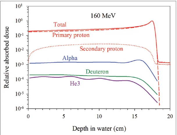
Explicit evaluation and theoretical modelling of nuclear interactions, as has been done for stopping and scattering processes, proves mathematically challenging. Their dose contribution is however signicantly low compared to that of primary protons (see Fig. 2.3) [58] [59]. In some analytical pencil beam algorithms, the eects of nuclear interactions on the total dose distribution are assumed to be small and of-ten accounted for by using measured depth-dose distributions. Studies previously

Figure 2.3: Depth-dose distribution for 160 MeV proton beam incident on a water phan-tom. Also plotted are the individual dose contributions of the primary protons and the secondary particles (Image from [60]).

conducted to investigate the inuence of nonelastic nuclear interactions on dose dis-tribution [58] [59] [60] show that nonelastic nuclear interactions remove primary protons from the incident beam, thereby decreasing the peak-to-plateau ratio of the total depth-dose distribution. Furthermore, generated secondary particles (except for neutrons) have short range and large scattering angles [1] [42]. Another inu-ence nonelastic nuclear interactions have on the depth-dose distribution, especially

(33)

2.3. Nuclear interactions 23 at high incident proton energies ('200 MeV), is a dose build-up eect observed in

the entrance region of the Bragg curve [61]. The build-up eect is partly caused by the Landau tails in the proton-electron energy transfer [35] (see Sec. 4.2). All these factors have to be included in a dose calculation algorithm if a more accurate result is to be achieved.

2.3.1 Including nuclear interactions in Geant4 simulations

With its exible framework for modular implementation of physics processes, the Geant4 toolkit is capable of putting together various kinds of hadronic interaction modules3_{. These modules describe the elastic scattering, inelastic scattering, nuclear}

interactions and the transport of secondary particles. In MC codes nuclear interac-tions are usually taken into account by using the total nonelastic nuclear interaction cross-section and branching ratios of dierent reaction channels liberating secondary particles [58]. In Geant4, hadronic interaction cross-sections are either tabulated, parameterized using analytical functions, or deduced from other cross-sections via general nuclear physics principles [58].

To model nonelastic nuclear interactions, one can assume an incident proton inter-acting with nucleons in the target nucleus, thereby liberating secondary nucleons and leaving the nucleus in an excited state (also known as the intra-nuclear cascade phase). Subsequently, the nucleus de-excites to equilibrium by emitting nucleons, and the residual nucleus can de-excite further (e.g., by evaporation) [48]. To simulate these processes, selected models are applied to dierent phases (e.g., intra-nuclear cascade, pre-equilibrium, and equilibrium) of the nuclear system as it evolves with time. Within the clinical energy range, the binary cascade and the Bertini cascade models for inelastic nuclear scattering of protons, neutrons, and heavier ions are known to give comprehensive description of the intra-nuclear cascade phase [48]. However, in the present work we follow the recommendations of Jarlskog et al. [48] and choose the binary cascade model over the Bertini cascade model for reasons that the latter gives a less accurate description of the target by considering it to have dis-continuous nuclear density distributions and potentials, uses entirely classical calcu-lation of scattering, is devoid of Coulomb barrier simucalcu-lation, and disregards nuclear momenta in calculations of reaction cross-sections. The binary cascade model also automatically invokes the G4PreCompoundModel (used to simulate the de-excitation of the nucleus in the pre-equilibrium phase) when energy of particles in the intra-cascade phase reaches a lower limit, whereas the Bertini intra-cascade model invokes its

3_{Note that term `module' is used here to refer to a collection of models that work together to}

(34)

2.3. Nuclear interactions 24 own `pre-equilibrium model', which is less accurate compared to the former [62] as shown by Quesada et al. [62]. At equilibrium, several de-excitation models are present (see Table 5.2) through the G4ExcitationHandler but for therapeutic pro-ton interaction with water the evaporation model (G4VEvaporation) is sucient [48]. Table 5.1 gives, among others, physics processes, models and data sets used in Geant4 to describe nuclear interactions.

(35)

Chapter 3 Simple proton beam congurations

In order to derive a satisfactory mathematical description of particle transport in matter, beam and geometric congurations must be explicitly dened. Sim-ple beam congurations range from pencil beams (sometimes referred to as point-monodirectional beams or beamlets [32]) to broad beams. Pencil beam here means that spatial and angular dimensions of the proton beam are innitesimally narrow at the point the beam impinges onto the medium. Similarly, in the plane-parallel beam congurations, individual proton pencil beams are assumed to be incident normally onto the plane surface of the medium. Simple beam congurations such as pencil beams are widely used in developing dose calculation algorithms for particle beams as they give a basis on which mathematical models for more realistic beam congurations can be derived [22].

3.1 Pencil beam kernels

The introductory part of the mathematical description of simple proton beam con-gurations is given in Appendix B.3. A pencil beam can be derived from the plane-parallel beam such as Eq. (B.3.3) by limiting the target surface area onto which the beam is incident. If we assume a narrow beam of monoenergetic particles incident on a small area δA=δxδy on thex−y plane at z = 0, the dose deposited by such

a pencil beam at some point~r in the medium can be written as Dpb(δA;~r) = Φ 0 pp Z Z δA Dpb E;x−x 0 , y−y0, z dx0dy0. (3.1.1)

Here, it is assumed that the energy spectrum of the source protons is uniform throughout the small area δA, i.e.,

Φ0_pp(x0, y0, E) = Φppψpp(E) ∀(x

0

, y0)∈δA, (3.1.2)

(36)

3.1. Pencil beam kernels 26 where Φpp and ψpp(E) are the uence and the normalized energy distribution of the initial protons respectively. Eq. (3.1.1) follows from Eq. (B.3.3) and is only valid for a homogeneous semi-innite medium, it is therefore a limiting case of a plane-parallel beam [63]. In Eq. (3.1.1), the pencil kernel Dpb is given by

Dpb(~r) = Z ∞

0

ψpp(E)Dpp(E;~r). (3.1.3) The dose deposited in the homogeneous semi-innite area Ω(z) (symmetric to the

initial beam direction) by each pencil beam can be summed up to approximate the dose of an arbitrary broad beam:

D(x, y, z) = Z Emax 0 dE Z Z Ω(z) Ψ E;x0, y0Dpb E;x−x 0 , y−y0, zdx0dy0. (3.1.4)

The integration is over the limits of the area Ω(z), conformal to the target volume,

onto which a collection of parallel PBs are incident normally [16]. The term Ψ

is the relative strength or energy uence of the PBs at x0, y0. It depends on the

incident proton energy, the material and the geometry of elements in the beamline. Therefore, algorithms used to calculate the energy uence usually involve modelling of the geometry and material of the beamline congurations, a topic beyond the scope of the current work. Hong et al. [17] developed such an algorithm to account for eects of elements upstream of the patient, and of the air gap between them and the patient, on the absorbed dose. The quantityDpbdenotes the dose distribution at the point ~r in the medium by the monoenergetic PB of energy E [16]. Throughout

the rest of this work we will refer to Dpb as the pencil beam kernel. The maximum penetration depth of the pencil beam kernel depends largely on the incident proton pencil beam energy and the density of the target [1]. It is however, independent of the eects of elements upstream of the target. The primary focus of this work is to model the three-dimensional proton pencil beam kernel Dpb.

At any arbitrary point p(x, y, z) = p(r, φ, z) in three-dimensional space, the PB

kernel takes the form

Dpb(E;x, y, z) = Dpb(E;r, φ, z) =Dpb(E;r,0, z) = Dpb(E;r, z) (3.1.5)

∀φ ∈ 0,2πand∀z ∈ _R.

Here, (r, φ, z) are the cylindrical coordinates, and r = px2 ₊_y2. The PB kernel

Dpb(r, φ, z) is radially symmetric about the z-axis or direction of propagation of the PB, therefore, does not depend on the azimuthal angle φ. Furthermore, Dpb can be written as a product of the depth dependent term g(z) and the o-axis term f(E;x, y, z) =f(E;r, z)[16] [17] [32] [18] as

(37)

3.2. Pencil beam kernel decomposition 27 The o-axis term f(x, y, z) describes the lateral spread of the primary proton PB

as a function of penetration depth, a phenomenon resulting from multiple Coulomb scattering (MSC) and range straggling [16] [1]. The depth-dependent term g(z)

corresponds to the central-axis of the broad beam measured in water. Therefore, it is usually obtained from measured depth dose distributions of broad beams in the water phantom [16] [17].

3.2 Pencil beam kernel decomposition

In this work we treat the total dose deposited in the medium as a sum of the contributions from three categories of particles: primary protons (pp), secondary protons (sp), and the rest of the particles and residual nuclei (e.g., deuterons, tritons,

α-particles, 3He) put together into a group we loosely call recoil (rc) ions. A similar

approach was taken in the dose calculation algorithm developed by Ulmer et al. [32] (see Ch. 4). Let us denote these categories of particles as:

1 = pp→primary protons, 2 =sp→secondary protons,

3 =rc→recoil and other secondary charged particles heavier than protons

(e.g., deuterons, tritons, α-particles, 3He).

The absorbed dose can therefore be decomposed into components corresponding to dose from each category of the interacting particles as follows (we will assume Dpb is implied (i.e., D=Dpb) as well as the dependence ofDpb onE, r and z)

D=Dpp+Dsp+Drc (3.2.1) = 3 X i=1 Di (3.2.2) = 3 X i=1 fi(E;r, z)gi(E;z), (3.2.3) wherefi(E;r, z)andgi(E;z)are the o-axis and the depth-dependent terms respec-tively, and the summation is over the three dierent category of particles (i= 1,2,3)

that are contributing to the total dose absorbed in the medium. We briey discuss here how each particle category contributes to the total absorbed dose:

3.2.1 Primary protons (pp)

These are protons originally incident on the medium and before they undergo nuclear interactions. Primary protons lose their energy only through Coulomb interactions,

(38)

3.2. Pencil beam kernel decomposition 28 in which a fraction of their energy is given to atomic electrons of the medium, leading to ionization (see Fig. 2.1) while part of it goes into atomic excitation and or dissociation [64] [21]. Due to the small electron to proton mass ratio, the energy transferred to each atomic electron at each interaction is generally quite small. Literature shows that the maximum energy transferred to knock-on electrons (δ−rays) never exceed 500 eV for 200 MeV protons [44] [43]. Overall, all of the energy

the proton loses in each electronic collision can be assumed to be deposited locally (at the site of interaction), hence contributing to the kernel component Dpp [15]. The loss of primary protons due to inelastic nuclear interactions causes reduction in primary proton uence, and is also taken into account by Dpp.

3.2.2 Secondary protons (sp)

Energy lost through inelastic nuclear interactions is transferred to uncharged parti-cles (neutrons and photons), secondary protons, and charged partiparti-cles heavier than protons, such as deuterons, tritons, 3_He_{, alpha particles and recoil nuclei [59] [56]}

[58] [65]. Secondary protons contribute ≈ 10% of the total dose proximal to the

Bragg peak of the unmodulated proton beam [58]. Occasionally, secondary particles undergo inelastic nuclear interactions, some of them yielding tertiary protons and several other tertiary particles. All protons produced in an inelastic nuclear interac-tion are referred to as `secondary protons' (Sec. 2.3), hence contribute to the dose component Dsp through the Coulomb interactions (as described above for primary protons). Secondary protons, p0_{, produced in elastic collisions such as} 1_H(p_,p0₎1_H0 contribute to Dsp through Coulomb interactions, while the recoil proton 1H0 (the recoil hydrogen nucleus) contribute to Drc.

3.2.3 Secondary neutrons and photons

Except through the emission of secondary protons in (n, pn) reactions, secondary neutrons do not signicantly contribute to the dose distribution as they interact further away from the point where they are emitted [59]. They are however, mainly responsible for the long tail beyond the distal edge of the Bragg peak [63]. This tail is insignicant relative to the Bragg peak. In the (n, pn) reactions, the dose that is deposited by p is assigned to Dsp, and that deposited by n to Drc. On the other hand, emission of secondary photons from inelastic nuclear interactions are negligible [15] [58]. In the current work the energy deposited by these photons was allocated to Drc.

(39)

3.2. Pencil beam kernel decomposition 29

3.2.4 Recoil and other secondary charged particles (rc)

The recoil and secondary charged particles heavier than protons (e.g., deuterons, tritons, α-particles, 3_He_{) are assumed to deposit most of their energy locally, hence}

their dose contribution to the total kernel D is through Drc [59]. Paganetti [58] shows that the energy deposited by these particles contribute less than 0.1% to the

total dose.

Let us now dene ρgi(z)dz as the average energy E¯i deposited at depths between

z and z + dz by primary protons (pp, i = 1), secondary protons (sp, i = 2),

and recoil ions and secondaries other than protons (rc, i = 3), where ρ is the

density of the medium. Also, let2πfi(r, z)rdrdenote fractions of the energyρgi(z)dz imparted to the medium by each particle category at radial distances between rand r+dr o the z-axis. The depth dependent components (also known as depth dose

distributions) gi(z) are given in units of MeV cm2/g (per source proton), while the o-axis components or radial dose distributions fi(r, z) are given in units of cm−2 [63]. We can also write

g(z) = 3

X i=1

gi(z) (3.2.4)

as the total energy-deposition distribution, so that

¯ E =ρg(z)dz = 3 X i=1 ¯ Ei (3.2.5)

is the average energy, per source proton, deposited in the medium at depths between

z andz+dzby all the radiation particles in the eld [63] [66]. The radial distribution fi(r, z) is dened by fi(r, z) =Di(r, z)/gi(z), (3.2.6) with ρ Z ∞ 0 g(z)dz =E0, (3.2.7) 2π Z ∞ 0 f(r, z)rdr = 1 ∀z >0, 2π Z ∞ 0 fi(r, z)rdr = 1 ∀z >0        , (3.2.8)

where E0 is the initial energy of the monoenergetic primary protons and i= 1,2,3

(the particle categories). It must be noted that the scattering is radially symmetric about the z-axis (or the direction of the pencil beam). Inserting Dpb(r, z) into Eq. (B.3.10), it can be shown, with the help of Eq. (3.2.7), that g(z) is equivalent to

(40)

3.2. Pencil beam kernel decomposition 30 the central-axis depth dose distribution of the broad parallel beam:

g(z) = lim

R→∞Dpp(R;z). (3.2.9) It follows immediately that

gi(z) = lim R→∞D

i