Student Sorting and Bias in Value Added Estimation:
Selection on Observables and Unobservables
by
Jesse Rothstein, Princeton University and NBER
CEPS Working Paper No. 170
June 2008
Acknowledgements: I thank Nathan Wozny and Enkeleda Gjeci for research assistance and the Industrial Relations Section and the Center for Economic Policy Studies at Princeton for financial support. I am grateful to the North Carolina Education Data Research Center and the North Carolina Department of Public Instruction for assembling and making available the data used in this study. This work has benefited from helpful conversations with Gordon Dahl, Ed Glaeser,
Student sorting and bias in value added estimation:
Selection on observables and unobservables
Jesse Rothstein∗
June 5, 2008
Abstract
Non-random assignment of students to teachers can bias value added estimates of teachers’ causal effects. Rothstein (2008) shows that typical value added models indi-cate large counter-factual effects of 5th grade teachers on students’ 4th grade learning, implying that assignments do not satisfy the imposed assumptions. This paper quanti-fies the resulting biases in estimates of 5th grade teachers’ causal effects from several value added models, under varying assumptions about the assignment process. Under selection on observables, models for gain scores without controls or with only a single lagged score control are subject to important bias, but models with controls for the full test score history are nearly free of bias. I consider several scenarios for selection on unobservables, using the across-classroom variance of observed variables to calibrate each. Results indicate that even well-controlled models may be substantially biased, with the magnitude of the bias depending on the amount of information available for use in classroom assignments.
∗Princeton University and NBER. Mailing address: Industrial Relations Section, Firestone Library,
Prince-ton, NJ 08544. E-mail: [email protected]. I thank Nathan Wozny and Enkeleda Gjeci for research assis-tance and the Industrial Relations Section and the Center for Economic Policy Studies at Princeton for financial support. I am grateful to the North Carolina Education Data Research Center and the North Carolina De-partment of Public Instruction for assembling and making available the data used in this study. This work has benefited from helpful conversations with Gordon Dahl, Ed Glaeser, Brian Jacob, David Lee, and Diane Schanzenbach, and from comments from Jane Cooley.
1
Introduction
Proposals to consider teacher quality in hiring, compensation, and retention require ade-quate measures of quality. This is increasingly defined in terms of educational outputs, as reflected in student performance, rather than by teacher inputs like graduate degrees and experience. In order for output-based quality measures to be of use, they must reflect teach-ers’causaleffects on the student outcomes of interest, not pre-existing differences among students for which the teacher cannot be given credit or blame.
If students were known to be randomly assigned to teachers, there would be no system-atic differences in students’ potential outcomes across teachers, so straightforward com-parisons of mean end-of-year achievement would provide unbiased estimates of teachers’ effects.1 But there is good reason to think that teachers are not in fact randomly assigned. Principals may attempt to group students of similar ability together, so as to permit more focused teaching to students’ skill levels, or they may try to spread high- and low-ability students across classrooms. Teachers who are thought to be particularly skilled at teaching, e.g., reading skills may be assigned students who are in need of extra reading help. Students who are known to create trouble together may be intentionally assigned to different class-rooms. Teachers who the principal would like to reward may be given the easiest-to-teach students, and teachers who the principal would like to induce to find another job may be given the troublemakers.2 Finally, parents, perceiving teacher assignments as important de-terminants of their children’s success, may intervene to ensure that their students are given 1There would still be the problem of accounting for sampling variation in the estimates: Because each
teacher is in contact with only a few dozen students per year, annual estimates of teacher effects are quite noisy, and compensation schemes based on these estimates would have to be robust to the mis-identification of teacher quality that results from this noise. But existing strategies – e.g., the Empirical Bayes approach used by Kane and Staiger (2008) or the similar Best Linear Unbiased Predictor used by the Tennessee Value Added Assessment System (Sanders and Horn, 1994) – suggest methods for doing this.
2This aspect of assignments is likely to depend on the accountability metric in place: If teachers are
re-warded for their value added and if value added estimates can be biased by systematic student assignment, the pattern of assignments is likely to change so that favored teachers benefit from this bias and disfavored ones are penalized.
a favored teacher or kept away from a disfavored one.
The evaluation challenge in teacher effect modeling is to distinguish teachers’ causal effects from the effects of pre-existing differences between the students in their classrooms. If the determinants of classroom assignments are not adequately controlled, teacher effect estimates will be biased. This bias is not averaged away even in large samples, and existing methods for adjusting value added estimates for sampling error will not (absent strong as-sumptions about, e.g., the across-year stability of teachers’ assignments) remove its effects from teacher rankings.
The premise of “value added” models is that differences in the difficulty of the task faced can be controlled by holding teachers responsible not for their students’ absolute end-of-year achievement but only for the students’ gains over the course of the year. Rothstein (2008) shows that this is false. Students are sorted across classrooms in ways that correlated not just with their score levels but also with their annual gains. Specifically, 4th grade gains are highly non-randomly sorted across 5th grade classrooms, with nearly as much across-class variation as in 5th grade gains. Because annual achievement tends to revert quickly toward a student-specific mean, a student with a 4th grade gain that exceeds the average by one standard deviation can be expected to fall short of the average in 5th grade by about 0.4 standard deviations. Existing value added models attribute this mean reversion to the 5th grade teacher. A teacher assigned students with high 4th grade gains in the previous year will look like a bad teacher through no fault of her own, while a teacher whose students posted poor gains in the previous year will be credited for their predictable reversion to trend.
Although Rothstein (2008) documents substantial non-randomness in teacher assign-ments that violates the restriction of common value added models (hereafter, VAMs), he does not directly estimate the magnitude of the resulting biases, and he provides little evi-dence about the prospects for correcting them via more sophisticated controls for students’
past achievement trends.3
This paper attempts to quantify the bias created by non-random assignment in several value added specifications. Three conditions govern the bias. It depends first on the amount of information available for use in the teacher assignment process about students’ potential end-of-year achievement or annual gain, second on the importance attached to this informa-tion in the formainforma-tion of teacher assignments, and third on the degree to which the control variables included in the value added specification can proxy for those used in assignments. I take the classroom effect – the causal effect of being in one classroom as opposed to another in the same school – as the parameter of interest.4 This avoids the problem of distinguishing different components of the classroom effect, the most obvious being the effects of teacher quality and of peers. This problem is complex, and is likely made even more difficult by non-random assignments of students to classrooms. But the identification of classroom effects is a necessary precondition for the larger problem of isolating teachers’ causal effects, and by focusing on this smaller, first problem I can place a lower bound on the bias in estimates of teachers’ effects that is produced by the assignment process.
Bias in classroom effect estimates can be measured directly if and only if classroom assignments are assumed to depend only on variables that are observed by the analyst, with random assignment conditional on these variables. Although I present estimates of this form, the selection-on-observables assumption is unattractive.
The bias created by selection on unobservables cannot be measured directly, but its magnitude can be quantified under assumptions about the amount and nature of information 3Rothstein (2008) does demonstrate that unbiased estimation requires controls fordynamicstudent
achieve-ment: Teacher assignments are not governed solely by permanent student characteristics, but respond dynami-cally to each year’s test scores. This rules out fixed effects solutions like those used by Harris and Sass (2006); Koedel and Betts (2007); Jacob and Lefgren (2008); Rivkin et al. (2005); and Boyd et al. (2007).
4Some value added studies use multiple cohorts of students assigned to each teacher. If assignments are
uncorrelated across cohorts – that is, if a teacher who gets high-potential-gain students this year is no more or less likely than any other teacher to get high-potential-gain students next year – then multiple cohort studies can convert bias in the classroom effect into mere sampling error in the teacher’s effect. But this uncorrelated assignments assumption is a strong one, and it does not appear to hold – even approximately – in the North Carolina data used here and in Rothstein (2008).
available to the principal for use in classroom assignments and about the way in which that information is used.5 The approach that I take is in the spirit of Altonji, Elder, and Taber’s (2005) assumption that sorting on unobserved variables resembles sorting on observables, though the specific assumptions differ: Where Altonji et al. (2005) assume that sorting is incidental and is equally correlated with observed and unobserved determinants of the outcome variable of interest, I assume that the sorting is intentional and that it depends on a limited set of predictors that are observed by the school principal, a subset of which are observed by the researcher as well. Altonji et al.’s assumption represents a limiting case for my analysis, in which the principal can perfectly predict students’ end-of-year achievement and gains before making teacher assignments.
Section 2 describes the data. In Section 3, I demonstrate that past test scores and behav-ioral variables are strongly predictive of future achievement and achievement gains. Section 4 summarizes the evidence from Rothstein (2008) that teacher assignments are importantly correlated with past scores. In Section 5, I compute and summarize the bias that arises in several common value added models if classroom assignments are random conditional on the observed variables. Section 6 develops the methodology for assessing the bias that would arise if the principal had more information about students’ potential learning growth than is available in research data sets. Section 7 presents the results of the analysis of bias with selection on unobservables. Section 8 concludes.
2
Data
I work with longitudinal administrative data on students in public elementary schools in North Carolina, assembled and distributed by the North Carolina Education Research Data Center. North Carolina has been a leader in the development of linked longitudinal data on 5For simplicity, I discuss class assignments as the outcome of principals’ decisions. This is not meant to
restrict the principal to be the only determinant of these assignments; the principal’s decision might reflect input from parents, teachers, and the student itself.
student achievement, and the North Carolina data have been used for several previous value added analyses (Clotfelter et al., 2006; Goldhaber, 2007).6
I focus on the value added of 5th grade teachers in 2000-2001. I use annual end-of-year tests that were given in grades 3-5, as well as “pre-test” scores given at the beginning of grade 3. I treat the pre-tests as 2nd grade tests.
The tests purport to use a so-called “developmental” scale, and the score scale is in-tended to be meaningful (i.e. scores are cardinal and not simply ordinal measures) both across grades and across the distribution within grades.7 I standardize scores so that the population mean is zero and the standard deviation one in 3rd grade; by using the same standardization in all grades I preserve the comparability of scores across grades.
The North Carolina data do not identify students’ teachers directly, but they do identify the person who administered the end-of-grade tests. In the elementary grades, this was usually the regular teacher. I follow Clotfelter et al. (2006) in using a linked personnel database to identify test administrators with regular teaching assignments. I count a match as valid if the test administrator taught a self-contained (all day, all subject) 5th grade class, if that class was not coded as Special Education or Honors, and if at least half of the tests that she administered were to 5th grade students. 73% of 5th grade tests were administered by teachers who are valid by this definition.
My analysis focuses reading scores, though similar results obtain for math scores. My sample consists of students who were in 5th grade in 2000-2001, who had a valid teacher assignment in that year, and for whom I have complete test score data in grades 3-5. Table 1A presents summary statistics and a correlation table for reading scores on the 3rd grade 6North Carolina was one of the first two states approved by the U.S. Department of Education to use
“growth-based” accountability models in place of the status-based metrics that are otherwise required under No Child Left Behind.
7It is not clear that a scale with this property is even possible (Martineau, 2006), or even if it is how one
would know whether a test’s scale has the property. Nevertheless, value added modeling as typically practiced is difficult to justify if scores do not have the so-called interval property. See Ballou (2002) and Yen (1986). The analysis here is not sensitive to violations of this property, though if it does not hold the value added estimators considered (here, and elsewhere in the literature) are difficult to justify. See Rothstein (2008).
pretest and on the end-of-grade tests in 3rd, 4th, and 5th grades, as well as for the 5th grade gain score (defined as the difference between the 4th and 5th grade scores). Mean scores in my complete-data sample are about 0.07 standard deviations higher than in the population in every grade. Scores are correlated about 0.80 in adjacent grades (lower for the 3rd grade pre-test, which is substantially shorter), with slightly reduced correlations across longer time spans. 5th grade gains are weakly positively correlated (+0.07) with 5th grade score levels and strongly negatively correlated (-0.52) with 4th grade scores. They are notably negatively correlated (-0.25) with 3rd grade scores as well.
Observed scores are noisy measures of true achievement. The degree of measurement error in test scores is usually measured by the “test-retest” reliability, the correlation be-tween students’ scores on alternative forms of the same test administered a short interval apart.8A 1996 report estimates that the test-retest reliability of the North Carolina 7th grade reading test is 0.86 (Sanford, 1996, p. 45). Unfortunately, test-retest studies have not been conducted for other grades. Under the assumption that individual item reliability is con-stant across grades and that item responses are independent, the 7th grade reliability can be extended to the shorter tests in earlier grades.9 Doing so, I estimate that the grade-3 pre-test has reliability 0.72, the grade-3 end-of-grade test has reliability 0.84, and the tests in grades 4 and 5 have reliability 0.86. I treat these as known, without sampling error.10
8Test makers often report alternative measures of reliability, e.g. internal consistency measures that are
based on correlations between a student’s scores on different subsets of questions. The internal-consistency reliabilities for the tests in grades 3, 4, and 5, respectively, are 0.92, 0.94, and 0.93 (Sanford, 1996, p. 45). The corresponding statistic for the grade-3 pre-test used for the cohort under consideration is not reported, but a more recent form of the test has reliability 0.82 (as compared with 0.92 in on the corresponding tests in grades 3-5; see Bazemore, 2004, p. 63). These statistics are computed under the assumption that responses are independent across questions; common shocks (e.g. a cold on test day) would lead these methods to overstate the test’s reliability.
9If item responses are not independent, reliability will be less sensitive to test length, and I will most likely
understate the reliability of the (relatively short) 3rd grade pretest.
10The sample for the test-retest study was only 70 students, in 3 classrooms. If the 70 observations are
independent, an approximate confidence interval for the grade-7 test reliability is (0.78, 0.91), though within-classroom dependence would imply a wider interval. Note also that a given test will have higher reliability in a heterogeneous population than in a homogeneous one; the likely homogeneity of the test-retest sample suggests that the reliability in the population of North Carolina students is probably higher than was indicated.
A known reliability allows me to compute summary statistics for true achievement, net of measurement error, assuming that errors are independent across grades. These are reported in Table 1B. The correlation between a student’s true achievement in grades g and g+1 is approximately 0.96. The 5th grade gain is negatively correlated with achievement levels in all grades.
One can examine across-grade correlations in gain scores as well as in score levels. The correlation between observed grade-4 and grade-5 gains is -0.42. Measurement error in the annual test scores biases this downward, but even when corrected the correlation re-mains negative. Thus, students with above-average gains in grade 4 will, on average, have below-average gains the following year. To the extent that such students are systemati-cally assigned to particular teachers, value added models that fail to account for this mean reversion will be biased against those teachers.
3
Predictions of grade 5 achievement and gains
Table 2 presents several specifications for students’ reading scores at the end of grade 5, using prior scores and other predetermined variables as explanatory variables. Because it is almost certainly more difficult to control for the sorting of students across schools than within, and because I focus in this paper in identifying differences in teachers’ effects within schools, I consider only specifications for within-school variation in 5th grade scores. The first column shows that 13% of the variance in 5th grade scores is across schools. Column 2 adds the 4th grade reading score. This has a coefficient of 0.680; neither zero (correspond-ing to a white noise process for individual scores) nor one (correspond(correspond-ing to a mart(correspond-ingale) is within the confidence interval. The inclusion of the 4th grade score increases the model’s R-squared by 0.55; 4th grade scores explain 63.5% of the within-school variation in 5th grade scores.
3. Both are significant predictors of 5th grade scores. Their inclusion lowers the 4th grade score coefficient by about one third, and raises the within-school R-squared by 0.045. Col-umn 4 adds three lagged scores on the math exam. Again, all are significant. The within-school R-squared is 0.058 higher than in the specification with just a single lagged reading score. Column 5 adds 28 additional covariates, measured in grade 4, that might help to predict students’ grade-5 achievement. These include race, gender, and free lunch sta-tus indicators; measures of parental education; various categories of “exceptionality” and learning disabilities; and measures of the time spent on homework and watching TV. These are jointly highly significant, though their inclusion raises the explained share of variance by only 0.003.
The available variables – all or nearly all of which would be readily observable when classroom assignments are made – explain nearly 70% of the within-school variation in students’ grade-5 test scores. Moreover, this substantially understates the predictability of student achievement. Recall from Section 2 that 14% of the variance in observed 5th grade scores is noise that would not even persist into a second administration of the test a week later. This noise is irrelevant to the predictability of achievement, and is uncorrelated with all predictor variables. Table 2 also shows estimates of the explained share of the within-school variance of true achievement, net of this transitory noise. These range from 0.764 with just the 4th grade score to 0.837 with the full set of controls.
Many value added models focus on the gain score rather than the end-of-year level. So long as the grade-4 score is included as a covariate, the coefficients in a prediction equation for (observed) gains are identical to those for levels, save that the grade-4 score coefficient is reduced by 1. The bottom rows of the Table show the R-squared statistics for specifications that take grade-5 gains as the dependent variable. These range from 0.279 to 0.398 within schools. The first-difference transformation reduces but does not eliminate predictability; the principal clearly has substantial information at his disposal for the prediction of student
gain scores.11
Also relevant to the analysis below is the value of past gains for predicting future scores and gains. Table 3 presents specifications using grade-4 gains as explanatory variables. These explain only 0.2% of the within-school variance in 5th grade achievement but 10.3% of the variance in 5th grade gains.
4
Evidence for non-random assignment
The simplest value added model estimates each teacher’s effect as the average gain score of her students. In order to attribute this average gain to the teacher, it must be the case that the information used to make teaching assignments is uninformative about students’ potential gains, conditional on any control variables. As shown in Section 3, prior achieve-ment and gains are strongly predictive of future scores and gains, so correlations between teacher assignments and past gains would violate the simple VAMs identifying assumption. Rothstein (2008) tests for “effects” of grade-gteachers on gains in gradeg−1. Given the evidence in Table 3, effects of this sort would indicate that expected grade-ggains are not balanced across grade-gclassrooms, and that the simple VAM will be biased.
LetAigbe the test score for studentiin gradeg. Then the student’s grade-ggain score is∆Aig≡Aig−Ai,g−1. The simple value added model specifies gain scores as depending
only on school (-by-grade) and teacher effects and random errors:12
∆Aig=Sigαg+Tigβg+εig, (1)
11The fit statistics cannot be directly converted to those that would be seen for the true gain score, net of
measurement error, because measurement error in the grade-4 score appears on both sides of the equation for grade-5 gains. I discuss in Section 6.4 how the coefficients of specifications for true gains can be recovered from the estimates in Table 2. True gains are quite predictable as well.
12This is essentially the specification used by the Tennessee Value Added Analysis System (Ballou et al.,
2004; Bock and Wolfe, 1996; Sanders and Horn, 1994, 1998; Sanders and Rivers, 1996; Sanders et al., 1997). Though TVAAS is estimated through a mixed effects framework, it implies equation (1)’s specification for gains, and it requires the same exclusion restriction.
whereSig andTig are vectors of indicators for students’ grade-g schools and teachers, re-spectively. The teacher effectsβg are normalized to have mean zero across all teachers in each grade at each school. The estimated effect of teacher jat schoolsis the average gain in classroom jless the average gain in the school:
ˆ
βg j = E[∆Aig|Tig= j,Sig=s]−E[Aig|Sig=s]
= βg j+E[εig|Tig= j,Sig=s]−E[εig|Sig=s]. (2)
If the mean of the error term distribution is the same for all teachers in the grade at the school,E[εig|Sig,Tig] =E[εig|Sig], this is unbiased.
This identifying assumption can be evaluated by examining gains in gradeg−1. The mean gain in gradeg−1 for students who will have teacher jin gradegis
E[∆Ai,g−1|Tig= j,Sig=s] =E[Si,g−1αg−1+Ti,g−1βg−1+εi,g−1|Tig= j,Sig=s]. (3)
Setting aside the first two terms, which might be absorbed through controls for the school attended and teacher assigned in gradeg−1, the grade-gteacher’s “effect” ong−1 gains is θj≡E[εi,g−1|Tig= j,Sig=s]−E[εi,g−1|Sig=s], the average grade-g−1 residual among
students in grade-gclassroom jless the average in schools.
If this is non-zero, the grade-geffect ˆβg jwill in general be biased. Suppose, for exam-ple, that theεprocess is autoregressive:εig=ρ εi,g−1+νig, whereνis serially uncorrelated
andνigis independent of the grade-gteacher assignment. Then
E[εig|j(i,g) = j,s(i,g) =s]−E[εig|s(i,g) =s] =ρ θj. (4)
Table 3 indicates thatρ=−0.39. Thus, any evidence thatθj is also non-zero would imply that the identifying assumption for the value added model (1) is violated.
I present estimates of 5th grade teachers’ coefficients in models for gain scores in grades 5, 4, and 3, using specifications like (1) and a balanced panel of students who attended the same school for all three grades. These are similar to those reported in Table 3 of Rothstein (2008), albeit estimated from a slightly different sample.
Begin with the model for grade-5 gains,
∆Ai5=Si5α5+Ti5β5+εi5. (5)
The 3,013 elements of the ˆβ5 vector (normalized to mean zero at the school) can be
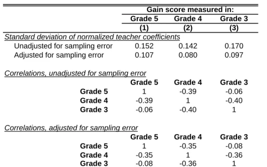
sum-marized by their standard deviation. This, 0.145, is shown in Column 1 of Table 4.13 I also report an adjusted standard deviation that subtracts from the across-teacher variance the contribution of sampling error to this variance (Aaronson et al., 2007; Rothstein, 2008). This adjusted standard deviation, which estimates the variability of the trueβ coefficients net of sampling error, is 0.106: A teacher who is one standard deviation better than average has students who gain 1/10 of a standard deviation (of achievement levels) relative to the average over the course of the year. This resembles existing estimates (Aaronson et al., 2007; Kane et al., forthcoming; Rivkin et al., 2005).
The remaining columns of Table 4 present counterfactual estimates that vary only the dependent variable. Column 2 presents estimates for 4th grade gains:14
∆Ai4=Si5α˜4+Ti5β˜4+ei4. (6)
We know that there are no causal effects of 5th grade teachers on 4th grade gains (i.e. 13Across-teacher means and standard deviations are weighted by the number of students taught, and degrees
of freedom are adjusted for the normalization of ˆβ5. Further details of the methods are available in Rothstein
(2008).
14In principle, the omission of controls for 4th grade teachers and schools creates an omitted variables bias
in (6). Rothstein (2008) presents estimates that include such controls. In practice, there is little correlation between teacher assignments in different grades, and estimates of the coefficients onT5in equations for
that ˜β4 =0), so any non-zero coefficients in this specification are indicative of student
sorting. The hypothesis that ˜β4 =0 is decisively rejected, and indeed there is nearly as
much variation in the elements of βˆ˜4 as in those of ˆβ5: The sampling-adjusted standard
deviation of 5th grade teachers’ normalized “effects” on 4th grade gains is 0.080, nearly as large as that for 5th grade gains. Column 3 presents an analogous model where the dependent variable is the 3rd grade gain, the difference between the student’s score on the end-of-grade reading test and the beginning-of-the year pretest. We see even larger apparent effects of 5th grade teachers here.
The lower portion of Table 4 presents correlations between the estimates of the coeffi-cient vectorsβ5, ˜β4, and ˜β3, first unadjusted for sampling error and then adjusted. Adjacent
coefficients are highly negatively correlated, both before and after the adjustment for sam-pling error, while there is nearly no correlation betweenβ5and ˜β3.
Two of these correlations are of particular interest here. First,corr
β5,β˜4
=−0.35. This indicates that 5th grade teachers who appear (by the simple model 5) to have high value added tend to be those whose students experienced below-average gains in grade 4. As noted earlier, gains are negatively autocorrelated at the student level; at least a portion of the variation in estimated 5th grade value added apparently reflects predictable consequences of non-random student assignments.
The second interesting correlation is that between ˜β4 and ˜β3, -0.36. One hypothesis
that could explain the presence of counterfactual “effects” of 5th grade teachers on earlier grades’ gains is that students differ systematically in their rate of gain, and that classroom assignments depend in part on that rate. Rothstein (2008) refers to this explanation as “static tracking”–the determinants of classroom assignments are constant across grades, and condi-tional on these determinants the test score in gradegdoes not affect the teacher assignment ing+1. In the presence of static tracking, the bias in teacher effects coming from non-random assignment can be absorbed by pooling data on a student’s gains across several
grades and including student fixed effects in the specification. This sort of specification is used by Harris and Sass (2006); Koedel and Betts (2007); Jacob and Lefgren (2008); Rivkin et al. (2005); and Boyd et al. (2007), among others.
As Rothstein (2008) notes, static tracking implies that in simple specifications like those in Table 4 the coefficients for the grade-gteacher on gains in gradeshandk(h,k<g) should be identical, up to sampling error. In other words,corr
˜ β4,β˜3
=1.15This restriction does not even approximately hold in the data. Classroom assignments are evidentlynot made on the basis of permanent student characteristics, but respond dynamically to annual stu-dent performance. This implies that stustu-dent fixed effects specifications provide inconsistent estimates of teachers’ causal effects. The only way to control for non-random classroom assignments while permitting consistent estimation of teachers’ effects is to measure the determinants of assignments directly.
Many value added specifications (Gordon et al., 2006; Kane et al., forthcoming; Aaron-son et al., 2007; Jacob and Lefgren, 2008) control for the baseline score, in effect modeling the end-of-year score as a function of the beginning-of-year score and the teacher assign-ment. These specifications are robust to dynamic teacher assignments of a very restricted form: Unless teacher assignments are random conditional on the baseline score, estimates will still be biased. The estimates in Tables 2 and 3 indicate that there is a great deal of information available to principals about students’ potential gains above and beyond that provided by the lagged score; there is no reason to expect that the use of this information in forming classroom assignments can be absorbed with simple controls. I show below that the once-lagged-score specification is rejected by the data.
15Again, this conclusion is supportable only if the correlation between ˜
β4and ˜β3is negative in specifications
that include controls for 4th and 3rd grade teachers, where those in Table 2 do not. The correlation is nearly identical when these controls are included.
5
Selection on observables
Strategies for isolating causal effects in the presence of non-random assignment of treatment (in this case, of classroom assignments) depend importantly on whether the determinants of treatment are observed or unobserved. In this section, I assume that 5th grade teacher assignments are random conditional on observable variables measured in 4th grade. Un-der this assumption, bias can be avoided by controlling for the full set of observables in the value added model. But models that use fuller controls may be biased if the included variables are unable to absorb all of the non-randomness of teacher assignments.
Note that no harm is done by controlling for variables that are not used in teacher assignments; this merely sacrifices some precision. Accordingly, I assume in this subsection thatXi,4is the set of variables included in Column 5 of Table 2 – the history of math and
reading test scores plus a set of demographic and behavioral variables as measured in grade 4. My baseline estimator for 5th grade teachers’ causal effects is:
∆Ai5=Si5α+Ti5β+Xi,4γ+εi js5. (7)
I estimate this by OLS, imposing the normalization that β have weighted mean 0 across teachers at each school. I compare the estimates that it yields to those from four value added models (hereafter,VAMs) with less-complete controls:
VAM1: Ai5 = Si5a+Ti5b+ei5
VAM2: ∆Ai5 = Si5a+Ti5b+ei5
VAM3: ∆Ai5 = Si5a+Ti5b+Ai4c+ei5
VAM4: ∆Ai5 = Si5a+Ti5b+Ai4c1+Ai3c2+Ai2c3+ei5
VAM1 credits each teacher with the average achievement of students in her class (less the school-level average). Few would advocate this “levels” specification. VAM2 credits each
teacher with her students’ average 5th grade gain score (again less the school average). This is the basic specification used in most value added policy and above in Section 4. VAM3 controls for students’ 4th grade achievement. Though I have written this as a model for the 5th grade gain, it is equivalent to a similar specification for the 5th grade score. VAM4 controls not just for last year’s score but for the two prior scores as well. This sort of specification is not widely used, but in principle it could be used in most value added implementations.
For each model, I compute the standard deviation across teachers of band of the bias relative to the coefficient vector from the richer specification (7). A useful summary statistic is the variance of the bias relative to that of teachers’ true effects, VV(b(−ββ)). I also compute the correlation between the bias and the true effect, corr(b−β,β): It is helpful to know whether good teachers (at least as indicated by the baseline model 7) are helped or hurt by the assignment process. A strong positive correlation between true effects and the bias would imply that teacher rankings are not much affected by sorting bias.
Table 5 presents the results. Each statistic is computed first from the estimated coeffi-cients (in the first panel), then adjusted for the influence of sampling error (second panel). The baseline specification indicates that the standard deviation of teachers’ effects is 0.096, or 0.124 before the adjustment for sampling error. VAM1 indicates much more variability of teacher effects, though this is primarily bias–the bias in this specification is more than three times as large (in variance terms) as the true variability that we are attempting to mea-sure. The specification for gain scores, VAM2, eliminates much of the bias, but its variance is still half that of the true effects. VAM3, controlling for the 4th grade score, cuts the stan-dard deviation of the bias in half; here, the variance of the bias is 13% of that of the quality signal. This is small in comparison with the previous models, but still substantial enough to represent a problem for policy. In each case, biases are only weakly correlated with true coefficients.
VAM4 eliminates nearly all of the bias relative to the richer selection-on-observables specification. This is unsurprising: Recall that Table 2 indicated that the control variables included in (7) but excluded from VAM4 added only 0.3% to the explained share of variance of grade-5 achievement and 0.6% to the explained share of variance of grade-5 gains. Thus, my assumption that specification (7) permits unbiased estimation of teachers’ causal effects implies that omitted variables bias in VAM4 is negligible. To understand the true potential for bias in this specification, we will need to consider the impact of selection on information that isunobservedin my sample but is available for use in forming classroom assignments. I develop methods for assessing this in the next Section.
6
A model of tracking on unobservables
There is no good reason to think that classroom assignments depend only on the variables available in my data. Indeed, the presence of noise in the observed test score history strongly suggests otherwise. Even a principal who had no additional information would almost cer-tainly be able to form a less noisy measure of students’ achievement each year by combining test scores with other measures (e.g. grades) that I do not observe. In this section I develop a framework in which classroom assignments depend on the observed variables and on unobserved variables that have known correlations with the observables. This permits com-putation of the variance across teachers of the bias in feasible estimates ofβ, though not the bias in any individual teacher’s estimated effect.
6.1 The sorting process
LetΩbe the information available to the principal for prediction of student outcomesY,
and letI =E[Y|Ω]be the best prediction that the principal can make given the available
information. Y might measure true gains or observed gains; we will see below that this has important consequences for the analysis. The amount of information available to the
principal about future gains can be measured byV(I)/V(Y)or, if we writeY =I+ε, by σ 2 I σI2+σε2
. The principal makes classroom assignments on the basis of an index λ =I+η. I represents the portion of the determinants of classroom assignment that are predictive of future achievement, whileηrepresents the remaining portion. I assume thatηis orthogonal to I, to all variables in the principal’s information set, Ω, and (by construction) to ε.16
I also assume that{I,η,ε}are jointly normally distributed. The importance of predicted outcomes in assignments is controlled byση2: If the principal assigns students to classrooms solely on the basis of predicted outcomes,ση2=0, while perfect random assignment can be seen as the opposite limiting case,ση2=∞.
Students are sorted perfectly onλ into classes. That is, all of the students assigned to a particular teacher have the sameλ value. This is a crude approximation at best. A typical school has three to five classes per grade; even if these classes are perfectly stratified,λ will have considerable heterogeneity within classes. The assumption of perfect sorting is made for reasons of mathematical tractability: With perfect sorting, we have simple expressions for, e.g., the across-class variance of I. With less than perfect sorting, my methods will understate the importance ofI (relative toη) in classroom assignments and therefore will understate the bias due to these assignments.17
6.2 Bias in undercontrolled value added models
The role of I in classroom assignments produces across-classroom differences in student achievement gains that do not reflect teacher quality, biasing value added models with inad-equate controls. It is easiest to characterize the bias in VAM2, which does not include any
16The assumption that
η is uncorrelated with observed predictors ofY is central to my strategy: I assume that the principal uses the observed variables solely to predictY, and does not sort students on the basis of these variables out of proportion to their information aboutY. This is required becauseΩ(and thereforeI) is only partially observable; I use the across-classroom share of variance of the observed test score history to recover
ση2.
17The basic approach could be extended to stratification on
λ across a finite number of classes (so that one class has students withλ ∈(−∞,c1), another hasλ ∈(c1,c2), etc.), at the cost of considerable additional
controls. Suppose thatY is the gain score, so that the principal makes classroom assign-ments on the basis of his predictions of the same outcome that is used to measure teacher effects. Then across-classroom differences inIrepresent biases inb. The across-classroom variance ofIisV(I)−V(I|λ) =corr2(I,λ)V(I) = σ
4 I σI2+ση2
.
In richer VAMs that include control variables,Z, these variables may absorb some of the bias. Write the regression ofIontoT andZasI=Tκ+Zπ+ν, whereTκis the remaining bias. Because λ is assumed to be perfectly sorted across classrooms, and because the teacher’s identity is informative aboutIonly throughλ, the teacher effectsTκsolely reflect differences across classes inλ, and we can therefore writeTκ=λ ξ andI=λ ξ+Zπ+ν. To obtain the coefficientsξ andπ, I assume that any variables available for use in the value added model are used by the principal to form his predictions (i.e.,Z⊆Ω), and are
orthogonal toη. The variance of the triplet(λ,I,Z)is thus
V λ I Z = σI2+ση2 σI2 cov(Z,I) σI2 σI2 cov(Z,I) cov(Z,I) cov(Z,I) V(Z) (8) and ξ π = V λ Z −1 cov(λ,I) cov(Z,I) = σI2+ση2 cov(Z,I) cov(Z,I) V(Z) −1 σI2 cov(Z,I) . (9)
There are thus three parameters that determine the variance of the bias in the under-controlled model, two deriving from the sorting process and one from the choice of value added specification. The first,σI2, concerns the principal’s ability to predict students’
out-comes. The second, ση2, controls the importance that the principal attaches to predicted outcomes in classroom assignments. The last describes the relationship between the control variables included in the value added model and the principal’s prediction,cov(Z,I). (A fourth parameter,V(Z), is readily measured.) With knowledge of these parameters, we can recoverξ and, via it,V(κ) =ξ2V(λ) =ξ2 σI2+ση2
.
To fix ideas, it is useful to consider three limiting cases. First, suppose that we control for all of the variables used by the principal (under selection on observables). ThenI=Zπ for someπ, ξ =0, andV(λ ξ) =V(Tκ) =0. Second, suppose that the principal places much more weight on variables unrelated to achievement than on predicted achievement in forming assignments, ση2 σI2. Then there is little sorting onI, ξ ≈0, andV(Tκ)≈ 0 regardless of the content of Z. Finally, suppose that the principal uses only predicted achievement to form assignments,ση2=0. Thenλ =I, and bias depends only on the extent to whichZcan account for the principal’s predictions. If there are noZvariables, bias will be in proportion to the principal’s ability to predict performance; withZvariables, bias will depend on the extent to which the econometrician can predict the principal’s predictions.
6.3 The principal’s prediction
Clearly, results concerning bias depend importantly on the information available to the prin-cipal for predictions of students’ future growth. In order to impose structure, I parametrise the principal’s information and its relationship with observed variables. I consider several scenarios. Intermediate cases between selection-on-observables and perfect predictability of future outcomes are the most realistic and I focus on these, though I also include the limiting cases for comparison. I begin with base cases in which selection is on observables, as in Section 5:
A. I=E[Y|Ag−1] =Ag−1φA: The principal has no information about future achievement
B. I=E[Y|A] =AφB, whereA= (A1, . . . . ,Ag−1)is the history of test scores up to grade
g−1. The principal observes the test score history, but has no additional information about achievement gains.
Note that scenarios A & B are falsified by the evidence in Table 2: Since the principal can observe all of the grade-4 variables that are available in my data, the fact that these variables are useful in predicting gains indicates that the principal has more information about poten-tial gains than just the score history. Nevertheless, these scenarios provide useful baselines. One use to which the principal might put his information is to reduce the noise that is contained in the test score history, A. Thus, a useful parametrisation of the princi-pal’s information assumes that he has access to k some number of additional series, un-observed by the researcher, that measure the true achievement history with independent, identically distributed error. That is, if the true achievement history through gradeg−1 is A∗=A∗1, . . . ,A∗g−1
andA=A∗+u, we can suppose that the principal observes in addi-tion{q1,q2, . . . ,qk}, whereqj=A∗+vj,E v0jvj =E(u0u), andE v0jvh =E v0ju =0. Theqseries can be thought of as representing grades, student evaluations, or classroom ob-servations that are available to the principal but not reported in typical data sets.
C. I=E[Y|A,q1, . . . ,qk] =AφC+q1τC1+q2τC2+. . .+qkτCk.
In the limit ask→∞, this scenario converges to one where the principal observesA∗without error:
D. I=E[Y|A∗,Ag−1] =A∗χD+Ag−1φD.
Note that I retainAg−1as a conditioning variable; whenY is the observed gain, the lagged
observed score can provide information about the error component inY (i.e. about∆Ag−
∆A∗g). By contrast, whenY is the true gain,φD=0.
These scenarios are quite restrictive. As we will see, the true achievement history ex-plains only 34% of the within-school variance of true achievement gains, and it is plausible
that the principal, who knows something of the child’s family situation and emotional and cognitive development patterns, has information about the remaining portion. LetW be a proxy for the principal’s information about∆A∗g−E
h ∆A∗g|A∗1, . . . ,A ∗ g−1 i . I assume without loss of generality thatWis orthogonal toA∗andu.
E. I=E[Y|A∗,Ag−1,W] =A∗χE+Ag−1φE+WψE.
Results here will depend on the quantity of information thatW is assumed to contain. I index this by f =V(WψE)/V(A∗χE). The limiting case (as f →V(∆A∗g|A∗)/V(A∗χE)18) is one in
which the principal can predict (true) gains perfectly:
F. I=Y.
This is not a particularly plausible scenario for the problem at hand, but it is useful for illustrating the relationship between the methods used here and those used by Altonji et al. (2005). Where in the earlier scenarios the principal observed all of the variables available to the analyst plus a subset of the remaining component of students’ gains, here the principal observes both components equally. As a result, both are equally sorted across classrooms. This does not imply perfect sorting on potential gains, as the principal may consider factors other than a student’s gain in forming classroom assignments. However, it does imply that selection on unobservables is identical to selection on observables, as in Altonji et al. (2005).19
The six scenarios are summarized in Table 6. 18This corresponds to f→1−R2
R2 , whereR
2is the explained share of variance from a regression of
∆A∗onto A∗. SinceR2is empirically about 0.34, this limit is just below 2.
19Altonji et al. also consider intermediate cases, where the correlation between the unobserved determinants
of selection and outcomes lies between zero (no selection) and the value corresponding to scenario F. The above framework can be seen as providing a basis for the choice of this correlation.
6.4 Calibration
Selecting a single scenario characterizing the principal’s information, observed covariances can be used to calibrate the model. There are three steps to the calibration: First, the coefficients entering into the principal’s prediction are estimated. This takes advantage of the observed relationship between gains and past scores, and of the structure that the various scenarios in Section 6.3 place on the principal’s predictions. Second, the degree of sorting of students to classrooms is computed, using as an input the measured between-classroom variance in observed predictor variables. Third, the bias in various value added models is computed.
6.4.1 Estimating the prediction coefficients
Table 2 presented estimates of theφ coefficients for scenarios A and B, whenY is the ob-served gain score. Estimates for predictions oftruegain scores, measured without error, can be computed using omitted variables formulae. The computation for scenario A illustrates the method. The observed gain,∆Ag, equals the true gain∆A∗gplus the difference between the measurement errors in the grade-g and grade-g−1 scores: ∆Ag=∆A∗g+ug−ug−1.
Because the test measurement error is independent across grades,ug cannot be predicted based on lagged variables. Butug−1 can, and the prediction coefficients can be obtained
by viewing the g−1 score,Ag−1, as a noisy measure of ug−1. Because the test error is
orthogonal to true achievement, E[Ag−1ug−1] =E
h
A∗g−1ug−1+u2g−1
i
=V(ug−1), and the
bias in a regression that takes∆Agas the dependent variable relative to one that uses∆A∗gis simply−V(ug−1)/V(Ag−1). Thus, theAg−1 coefficient from a model for true gains equals the
Ag−1 coefficient from a model for observed gains (Table 2, column 2) plusV(ug−1)/V(Ag−1).
A multivariate version of this yields coefficients for scenario B when Y is the true gain. Similar methods can be used to recover the coefficients in scenarios C and D, for either definition ofY. Begin with scenario D whenY is the true gain. We have already discussed
a method for obtaining φB, the coefficients of a regression of true gains on the observed score history,A. A standard errors-in-variables formula relates these to the coefficients for predictions of true gains from the true achievement history,χD:
φB=
I− EAA0−1Euu0
χD. (10)
Inversion of this formula provides an expression forχD. It is straightforward to extend this to the case whereY is instead theobservedgain.
Now consider scenario C, where the principal observes k+1 noisy measures of the achievement history but not the history itself. IfY is the true gain, the principal’s best prediction will use the average of his measures, ¯A= k+11 A+q1+. . .+qk. The variance of the measurement error in this average will equal k+11 times the variance of the error in a single series. Thus, whenk+1 series are available the coefficients for each series will be
φC=τC1=. . .=τCk= 1 k+1 I− 1 k+1 E AA0−1Euu0 χD. (11)
(Note that this is identical to (10) whenk=0.) WhenY is instead the observed gain, the coefficients on the observed history will deviate from those for the kother histories. The correction for the presence of correlated measurement error in the dependent variable and one of the independent variables is again straightforward.
Scenarios E and F differ, in that not all of the coefficients can be estimated directly. Assumptions about f, the ratio of the principal’s information about the component of gains that is orthogonal to the achievement history to the information contained in that history, replace estimates of the prediction coefficientsψ. χandφare as in scenario D.
6.4.2 Recovering the sorting parameters
With estimates of coefficients for predictor variables with known variance, it is trivial to compute σI2. The next step is to estimate the extent to which students are sorted across classrooms on the basis of I. I assume that there is some uni-dimensional student-level statisticω that is observable to the researcher and is contained withinΩ(so orthogonal to
η). Empirically, I use linear combinations of past test scores forω.20 The various scenarios pin downcov(I,ω). We can recover ση2 by analyzing the between-classroom variance of ω. The within-classroom variance is
V(ω|λ) = V(ω) 1−corr2(ω,λ) (12) = V(ω)−cov 2( ω,λ) V(λ) (13) = V(ω)−cov 2( ω,I) σI2+ση2 . (14) Rearranging terms, we obtain
ση2= cov
2(ω,I)
V(ω)−V(ω|λ)−σ
2
I. (15)
Note that the denominator here is simply the across-class variance ofω.
6.4.3 Computing the bias
I consider value added models VAM2, VAM3, and VAM4 from Section 5. These are dis-tinguished by the control variables that are included in models for the grade-ggain. In each case, the control variables are subsets of theAvector, so it is straightforward to compute the covariance between these variables and the principal’s prediction. As indicated by equation 20I weight past scores based on the weights applied to either true or observed achievement in the principal’s
(9), this is sufficient to compute the variance of the bias term,V(Tκ).21
7
Results
7.1 The principal’s prediction
Table 2 presented prediction models for the grade-5 test score as a function of test scores in earlier grades. As discussed above, these are readily converted into predictions of grade-5 gains given the observed achievement history. Columns 1 and 2 of Table 7 present the prediction coefficients, when the predictor variables are the 4th grade reading score (column 1) or the sequence of three prior reading scores (column 2).
These models overstate the value of prior test scores for predicting true gains, net of measurement error. This is because the noisy 4th grade test score achieves predictive power for the observed 5th grade gain due to the presence of the same measurement error, u4,
in both variables. As discussed above, standard errors-in-variables formulae can be used to obtain the best prediction equations for true gains. These are presented in columns 3 and 4 of Table 7.22 The within-school R2 statistics and especially the prediction coef-ficients themselves are reduced in magnitude from the specifications for observed gains. True achievement gains are negatively correlated with past achievement levels, but not dra-matically so.23 The model for observed gains in column 2 implicitly attaches a coefficient of around -0.81 (=−0.57−0.24) to the 4th grade gain, while the corresponding model for true gains assigns a weight of only -0.02 (=−0.07− −0.05) to this gain.
Table 8 presents estimates of the coefficients that the principal would apply to the avail-able predictor variavail-ables in scenarios C and D. Columns 1-4 show prediction coefficients 21Extending the analysis to VAMs that control for non-test variables requires assumptions about the
relation-ship between these variables and theqandW variables seen by the principal. I do not pursue this here.
22In principle, the coefficients of regressions that include math scores could be recovered as well.
23Note that this implies that value added models which impose a coefficient of 1 on the lagged achievement
for observed gains, while columns 5-8 show coefficients for true gains. Columns 1 and 5 repeat the coefficients from scenario B, where only the observed test score history is avail-able. Columns 2 and 6 show coefficients when a second, equally noisy series is availavail-able. Columns 3 and 7 show coefficients when two series are available in addition to observed scores (i.e. k=2). Note that the coefficients on the observed and unobserved series are identical in columns 6 and 7, where the dependent variable is the true gain, but that they differ in columns 2 and 3, where the observed series can be used to predict some of the mea-surement error in the observed gain. Columns 4 and 8 show predictions assuming that the principal is able to observe the history of true achievement. This substantially improves his ability to predict observed gains, as the measurement error portion of the 4th grade score can be perfectly isolated, but adds relatively little to his ability to predict true gains over what could be done with three noisy histories.
7.2 The importance of predictions in classroom assignments
Using the coefficients from Tables 2, 7, and 8 and relying on an observed component of the principal’s predictions, I can compute the variance decomposition of the principal’s predictions,I, into within- and between-classroom components. For scenario C, I present estimates fork=1 andk=2. In scenario E, I present estimates for f =0.25, f =0.5, and
f =1; the scenario of perfect information, F, corresponds to f =1.96.
The first column of Table 9 shows the fraction of the within-school variance in gains that the principal is able to predict (i.e. σI2/V(Y)) in each scenario, for true gains in the first
panel and for observed gains in the second panel. The second column shows the across-school share of variance for the scenarios in whichI is perfectly observable. Coefficients for between-school predictions may differ from those for the within-school predictions that I focus on, so I do not compute the across-school component of the incompletely observed indices. Column 3 shows the fraction of the within-school variation that is across
class-rooms. This equals σI2 σI2+ση2
, the weight placed on predicted outcomes relative to other fac-tors in classroom assignments. Column 4 shows the across-classroom standard deviation in predicted gains.
Not surprisingly, the scenarios in which the principal has more information permit him to explain a larger share of the within-school variance in gains. Moreover, the richer predic-tion scenarios yield larger estimates of the across-classroom share of variance of predicted gains. Thus, the more information that we permit the principal to have about the student’s achievement history, the larger is the bias that is implied for value added specifications (like VAM2) that do not allow for across-classroom sorting.
Sorting appears to be substantially more important when the principal is presumed to be using predictions of observed rather than true gains for classroom assignments. But this can be misleading: True gains are much less variable than observed gains (with a standard deviation less than half as large). Disparities between the panels are smaller in column 3, showing the fraction of the variance of predicted gains that is across classrooms. Even in this column, though, scenarios C-E show more sorting in the second panel. This is because observed scores form a smaller share of predicted observed gains than of predicted true gains in these scenarios (compare the R-squared statistic in column 1 of Table 8 to those in columns 2-4, versus that in column 5 and those in 6-8), so the same sorting on observed variables corresponds to more overall sorting in the observed gain scenarios.
7.3 Bias in value added models with controls for observables
Table 9 shows that the standard deviation of across-classroom differences in predicted gain scores ranges from 0.037 to 0.191, depending on the assumptions made about the informa-tion used in sorting. This variainforma-tion is bias in specificainforma-tions like VAM2 that do not control for classroom assignments. By comparison, the total across classroom standard deviation of observed gain scores is 0.134. Thus, even scenarios that restrict the principal to use little
more than the observed variables in classroom assignments indicate biases in simple value added models that are large relative to the effects that we hope to measure.
Table 10 presents estimates of the standard deviation of the bias in richer models that include controls for students’ prior achievement. Columns 1-3 of this table index value added models, corresponding to VAMs 2, 3, and 4, respectively. The bias in the simplest model (VAM2) is substantial in every scenario. Column 2 shows that the inclusion of a control for the prior year’s test score eliminates much of the bias in VAM2, though there is important variation across scenarios. If we assume that the principal forms classroom assignments on the basis of his predictions of true gains (rather than observed gains)and that he has no information about students’ potential gains beyond that contained in their achievement histories (as in scenarios B-D), the remaining bias in VAM3 is negligible. However, if we allow the principal to have additional information or if we assume that he sorts on the basis of predictedobservedgains – as he likely would if accountability policies condition rewards and punishments on observed gains rather than on unmeasurable true gains – then the bias remains important. If the principal observes even two independent achievement histories (e.g. the test score history plus an additional series, perhaps coming from teacher grades) and uses them in classroom assignments, the standard deviation of the bias in VAM3 is 0.043.
Column 3 shows that much of the bias in VAM3 remains in VAM4, which controls for the full sequence of prior test scores. If the principal is assumed to observe the student’s true achievement history plus another set of variables that explain an equal amount of student gains (i.e. scenario E with f =1), the standard deviation of the bias ranges from 0.051 to 0.076, both large relative to the standard deviation of teachers’ estimated “effects.”
8
Conclusion
Typical value added analyses treat the process by which students are assigned to teachers as ignorable, under the implicit assumption that the statistical model used can absorb any sys-tematic non-random assignment. This would be true if, for example, classroom assignments were random conditional on students’ prior-grade test scores. But there is little reason to think that this is an adequate characterization of classroom assignments. Principals have a great deal of information beyond the prior test score that is predictive of students’ end-of-year achievement, and this information is unlikely to be ignored in classroom assignments. This paper attempts to quantify the bias that arises in value added models that fail to control for the determinants of classroom assignments. The task is straightforward if class-room assignments are assumed to be random conditional on observable variables. My anal-ysis indicates that simple VAMs that fail to control for the dynamic process of test scores, simply modeling differences in mean gain scores across classrooms, are substantially bi-ased by student sorting. The bias is reduced – with a variance about 15% as large as that of teachers’ true effects – in a VAM that controls for the lagged score, and is further reduced when additional lagged scores are included as controls.
The analysis is more complex if we loosen the unrealistic assumption that all of the information considered by the principal in forming teacher assignments is available in the research dataset. I develop methods for assessing the bias when the principal is assumed to have access to a limited amount of information that the researcher cannot observe. I consider several scenarios for the information set, and estimate the bias in three value added models under each scenario.
A great deal turns out to depend onhowthe principal uses his information: If he weights past achievement to best predict observed gains, even a limited amount of unobserved infor-mation generates substantial biases in the sorts of value added models that are commonly used. Richer models that control the full test score history rather than just a single lagged
score reduce these biases, but only if the principal has very limited information about stu-dents’ potential. With less restrictive assumptions, biases remain quantitatively important even in rich value added models.
Three recent studies have provided evidence that appears to validate observational value-added estimates. On closer examination, however, all are consistent with the presence of substantial bias in these estimates. Jacob and Lefgren (2008) and Harris and Sass (2007) compare value added estimates with principals’ subjective assessments of teacher quality, which might be assumed to reflect unbiased estimates of teachers’ causal effects. Both pa-pers find that the two measures are correlated, though far from perfectly. This indicates that there is at least some signal in the value added estimates. But the weak correlations leave plenty of room for non-causal factors in the VAM estimates.
Kane and Staiger (2008) compare estimates of teacher effects from a randomized ex-periment with observational estimates based on data prior to the exex-periment. They test the hypothesis that the (appropriately shrunken) observational estimate is an unbiased predic-tion of the causal estimate, and obtain estimates consistent with this hypothesis. There are three important sources of slippage here. First, Kane and Staiger test a statistical hypothesis about the joint distribution of the true coefficients and the bias; while zero bias is consistent with the null hypothesis, so are large biases that are negatively correlated with teachers’ true causal effects.24 Second, Kane and Staiger’s sample provides low power. Their standard errors are consistent with substantial attenuation of the prediction coefficient due to bias in the observational estimates. While their confidence intervals might rule out my scenario F (if biases are assumed to be uncorrelated with true quality), my more realistic scenarios are wholly consistent with the Kane and Staiger estimates but are nevertheless extremely troubling regarding the potential for bias in value added estimates. Finally, the Kane and
24They test the hypothesis that cov(β,b)
V(b) =1, whereβ is the vector of causal effects andbis the best linear
predictor ofβ+κ, the sum of causal effects and any bias, based on the coefficients from the value added model.
Staiger analysis is based on a carefully selected sample of pairs of teachers for which prin-cipals consented to random assignment. One might expect that principal consent was more likely when the two teachers would have been given similar students in any case. If so, the results cannot be generalized beyond the sample, even to other teachers at the same schools. The results here suggest that it is hazardous to interpret typical value added estimates as indicative of causal effects. Although some assumptions about the assignment process permit nearly unbiased estimation, other plausible assumptions yield large biases. Further evidence on the process by which students are assigned to classrooms is needed before it will be clear which types of assumptions are closest to reality. The most recent such study, Monk (1987), is now more than twenty years old. More recent evidence, from studies more directly targeted at the assumptions of value added modeling, is badly needed, as are richer VAMs that can account for real world assignments. In the meantime, causal claims will be tenuous at best.
References
Aaronson, Daniel, Lisa Barrow, and William Sander, “Teachers and Student
Achieve-ment in the Chicago Public High Schools,”Journal of Labor Economics, January 2007, 24(1), 95–135.
Altonji, Joseph G., Todd E. Elder, and Christopher R. Taber, “Selection on observed
and unobserved variables: Assessing the Effectiveness of Catholic Schools,”Journal of
Political Economy, February 2005,113(1), 151–184.
Ballou, Dale, “Sizing Up Test Scores,”Education Next, Summer 2002,2(2), 10–15.
, William Sanders, and Paul Wright, “Controlling for Student Background in
Value-Added Assessment of Teachers,” Journal of Educational and Behavioral Statistics, Spring 2004,29(1), 37–65.
Bazemore, Mildred, “North Carolina Reading Comprehension Tests,” Technical Report
(Citable Draft), Office of Curriculum and School Reform Services, North Carolina De-partment of Public Instruction. September 22, 2004.
Bock, R. Darrell and Richard Wolfe, “Audit and review of the Tennessee Value-Added Assessment System (TVAAS),” Final Report, Office of Education Accountability, Comptroller of the Treasury. March 1996.
Boyd, Donald, Hamilton Lankford, Susanna Loeb, Jonah E. Rockoff, and James
Wyckoff, “The Narrowing Gap in New York City Teacher Qualifications and Its
Im-plications for Student Achievement in High-Poverty Schools,” Working Paper 10, Center for Analysis of Longitudinal Data in Education Research. September 2007.
Clotfelter, Charles T., Helen F. Ladd, and Jacob L. Vigdor, “Teacher-Student Matching
and the Assessment of Teacher Effectiveness,”Journal of Human Resources, Fall 2006, 41(4), 778–820.
Goldhaber, Dan, “Everyone’s Doing It, But What Does Teacher Testing Tell Us About
Teacher Effectiveness?,” Working Paper 9, Center for Analysis of Longitudinal Data in Education Research. April 2007.
Gordon, Robert, Thomas J. Kane, and Douglas O. Staiger, “Identifying Effective
Teach-ers Using Performance on the Job,” Discussion Paper 2006-01, The Hamilton Project. April 2006.
Harris, Douglas N. and Tim R. Sass, “Value-Added Models and the Measurement of
Teacher Quality,” April 2006. Unpublished manuscript.
and , “What Makes for a Good Teacher and Who Can Tell?,” July 2007. Unpublished manuscript.
Jacob, Brian A. and Lars Lefgren, “Can Principals Identify Effective Teachers? Evidence
on Subjective Performance Evaluation in Education,”Journal of Labor Economics, Jan-uary 2008,25(1), 101–136.
Kane, Thomas J. and Douglas O. Staiger, “Are Teacher-Level Value-Added Estimates
Biased? An Experimental Validaton of Non-Experimental Estimates,” March 17, 2008. Unpublished manuscript.
, Jonah E. Rockoff, and Douglas O. Staiger, “What Does Certification Tell Us About
Teacher Effectiveness? Evidence from New York City,”Economics of Education Review, forthcoming.
Koedel, Cory and Julian R. Betts, “Re-Examining the Role of Teacher Quality in the
Edu-cational Production Function,” Working paper 07-08, University of Missouri Department of Economics April 2007.
Martineau, Joseph A., “Distorting Value Added: The Use of Longitudinal, Vertically
Scaled Student Achievement Data for Growth-Based, Value-Added Accountability,” Journal of Educational and Behavioral Statistics, Spring 2006,31(1), 35–62.