Spectral Methods for Numerical Relativity

Spectral Methods for Numerical Relativity

Philippe Grandclement, J´

erˆ

ome Novak

To cite this version:

Philippe Grandclement, J´

erˆ

ome Novak. Spectral Methods for Numerical Relativity. This paper

has bene submitted to Living Reviews in Relativity. All comments are welcomed before i.. 2007.

<

hal-00155093v1

>

HAL Id: hal-00155093

https://hal.archives-ouvertes.fr/hal-00155093v1

Submitted on 15 Jun 2007 (v1), last revised 23 Jan 2008 (v2)

HAL

is a multi-disciplinary open access

archive for the deposit and dissemination of

sci-entific research documents, whether they are

pub-lished or not.

The documents may come from

teaching and research institutions in France or

abroad, or from public or private research centers.

L’archive ouverte pluridisciplinaire

HAL

, est

destin´

ee au d´

epˆ

ot et `

a la diffusion de documents

scientifiques de niveau recherche, publi´

es ou non,

´

emanant des ´

etablissements d’enseignement et de

recherche fran¸cais ou ´

etrangers, des laboratoires

publics ou priv´

es.

hal-00155093, version 1 - 15 Jun 2007

Spectral Methods for Numerical Relativity

Philippe Grandcl´

ement

Laboratoire Univers et Th´

eories

UMR 8102 du C.N.R.S., Observatoire de Paris

F-92195 Meudon Cedex, France

email: [email protected]

http://www.luth.obspm.fr/minisite.php?nom=Grandclement

J´

erˆ

ome Novak

Laboratoire Univers et Th´

eories

UMR 8102 du C.N.R.S., Observatoire de Paris

F-92195 Meudon Cedex, France

email: [email protected]

http://www.luth.obspm.fr/minisite.php?nom=Novak

Abstract

Equations arising in General Relativity are usually to complicated to be solved analyti-cally and one has to rely on numerical methods to solve sets of coupled, partial differential, equations. Amongst the possible choices, this paper focuses on a class called spectral meth-ods where, typically, the various functions are expanded onto sets of orthogonal polynomials or functions. A theoretical introduction on spectral expansion is first given and a particular emphasize is put on the fast convergence of the spectral approximation. We present then different approaches to solve partial differential equations, first limiting ourselves to the one-dimensional case, with one or several domains. Generalization to more dimensions is then discussed. In particular, the case of time evolutions is carefully studied and the stability of such evolutions investigated. One then turns to results obtained by various groups in the field of General Relativity by means of spectral methods. First, works which do not involve explicit time-evolutions are discussed, going to rapidly rotating strange stars to the computation of binary black holes initial data. Finally, the evolutions of various systems of astrophysical interest are presented, from supernovae core collapse to binary black hole mergers.

1

Introduction

Einstein’s equations represent a complicated set of nonlinear partial differential equations for which some exact [23] or approximate [24] analytical solutions are known. But these solutions are not always suitable for some physically or astrophysically interesting systems, that require an accurate description of their relativistic gravitational field, without any assumption on the symmetry or with the presence of matter fields for instance. Therefore, many efforts have been undertaken to solve Einstein’s equations with the help of computers in order to model relativistic astrophysical objects. Within this field of numerical relativity, several numerical methods have been experi-mented and a large variety of them are currently being used. Among them,spectral methods are now increasingly popular and the goal of this review is to give an overview (at the moment it is written or updated) of the methods themselves, the groups using them and the obtained re-sults. Although some theoretical framework of spectral methods is given in Secs. 2 and 3, more details about spectral methods can be found in the books by Gottlieb and Orszag [68], Canutoet al.[44, 45, 46], Fornberg [61] and Boyd [39]. While these references have of course been used for writing this review, they can also help the interested reader to get deeper understanding of the subject. This review is organized as follows: hereafter in the introduction, we briefly introduce the spectral methods, their usage in computational physics and give a simple example. Sec. 2 gives important notions concerning polynomial interpolation and the solution of ordinary differential equations (ODE) with spectral methods. The cases of partial differential equations (PDE), includ-ing time evolution or several spatial dimensions, are treated in Sec. 3. The last two sections are then reviewing results obtained using spectral methods: on stationnary configurations and initial data (Sec. 4), and on the time-evolution (Sec. 5) of stars, gravitational waves and black holes.

1.1

About Spectral Methods

When doing simulations and solving PDE, one faces the problem of representing and manipulating functions on a computer, which deals only with (finite) integers. Let us take a simple example of a functionf : [₋1,1]_→R_{. The most straightforward way to approximate it is through}

finite-differences methods: first one must setup agrid

{xi}i=0...N ⊂[−1,1]

ofN+ 1 points in the interval, and representf by itsN + 1 values on these grid points

{fi=f(xi)}_i=0...N.

Then, the (approximate) representation of the derivativef′ _{shall be, for instance}

∀i < N, fi′=f′(xi)≃ fi+1−fi

xi+1−xi. (1)

If we suppose an equidistant grid, so that ∀i < N, xi+1 −xi = ∆x = 1/N, the error in the

approximation (1) will decay as ∆x(first-order scheme). One can imagine higher-order schemes, with more points involved for the computation of each derivative and, for a scheme of ordern, the accuracy will go as (∆x)n= 1/Nn_.

Spectral methods represent an alternate way: the function f is no longer represented through

its values on a finite number of grid points, but using its coefficients (coordinates)_{ci}i=0...N in a

finite basis of known functions_{Φi}i=0...N

f(x)_≃

N X

i=0

A relatively simple case is, for instance, when f(x) is a periodic function of period 2, and the Φi(x) = cos(πix),sin(πix) are trigonometric functions. Eq. (2) is then nothing but the truncated

Fourier decomposition off. In general, derivatives can be computed from theci’s, with the

knowl-edge of the expression for each derivative Φ′

i(x) as a function of{Φi}i=0...N. The decomposition (2)

is approximate in the sense that _{Φi}i=0...N represent a complete basis of some finite-dimension

functional space, whereasf usually belongs to some other infinite-dimension space. Moreover, the coefficientsci are computed with finite accuracy. Among the major advantages of using spectral

methods is the exponential decay of the error (ase−N_{), for well-behaved functions (see Sec. 2.4.3);}

one therefore has aninfinite-order scheme.

In a more formal and mathematical way, it is useful to work with the methods of weighted residuals (MWR, see also Sec. 2.5). As in that section, let us consider the PDE

Lu(x) = s(x) x_∈U _⊂Rd_{, (3)}

Bu(y) = 0 x_∈∂U, (4)

where L is a linear operator,B the operator defining the boundary conditions and s is a source term. A function ¯u is said to be a numerical solution of this PDE if it satisfies the boundary conditions (4) and makes “small” the residual

R=Lu¯₋s. (5)

If the solution is searched in a finite-dimensional subspace of some given Hilbert space (any relevant

L2U space) in terms of the expansion (2), then the functions{Φi(x)}i=0...N are calledtrial functions

and, in addition the choice of a set oftest functions {χi(x)}i=0...N defines the notion of smallness

for the residual by means of the Hilbert space scalar product

∀i= 0...N, (χi, R) = 0. (6)

Within this framework, various numerical methods can be classified according to the choice of the trial functions:

• Finite differences: the trial functions are overlapping local polynomials of low order,

• Finite elements: the trial functions are smooth functions which are non-zero only on subdomains ofU,

• Spectral methods: the trial functions are global smooth functions onU.

Various choices of the test functions define different types of spectral methods, as detailed in Sec. 2.5. Usual choices for the trial functions are (truncated) Fourier series, spherical harmonics or orthogonal families of polynomials.

1.2

Spectral Methods in Physics

We do not give here all the fields of physics where spectral methods are being employed, but we sketch the variety of equations and physical models that have been simulated with such techniques. Spectral methods originally appeared in numerical fluid dynamics, where large spectral hydrody-namics codes have been regularly used to study turbulence and transition, since the seventies. For fully resolved, direct numerical calculations of Navier-Stokes equations, spectral methods were of-ten preferred for their high accuracy. Although high-order finite-difference codes can yield similar accuracy, spectral methods still have an advantage because they permit fast, direct solution of Poisson’s equation. Solving Poisson’s equation is required to determine the pressure gradient that appears in the Navier-Stokes equations. Historically, they also allowed for two- or three-dimensional

simulations of fluid flows, because of their reasonable computer memory requirements. Many ap-plications of spectral methods in fluid dynamics have been discussed by Canutoet al.[44, 46], and the techniques developed in that field can be of some interest for numerical relativity.

From pure fluid-dynamics simulations, spectral methods have rapidly been used in connected fields of research: geophysics [130], meteorology and climate modeling [146]. In this last domain of research, they provide global circulation models that are then used as boundary conditions to more specific (lower-scale) models, with improved micro-physics. In this way, spectral methods are only a part of the global numerical model, combined with other techniques to bring the highest accuracy, for a given computational power. Solution of the Maxwell equations can, of course, be also obtained with spectral methods and therefore, magneto-hydrodynamics (MHD) have been studied with these techniques (seee.g. Hollerbach [84]). This has been the case in astrophysics too, where for example spectral three-dimensional numerical models of solar magnetic dynamo action realized by turbulent convection have been computed [42]. Still in astrophysics, the Kompaneet’s equation, describing the evolution of photon distribution function in a bath of plasma at thermal equilibrium within the Fokker-Planck approximation, has been solved using spectral methods to model the X-ray emission of Her X-1 [26, 32]. In the simulations of cosmological structure formation or galaxy evolution, many N-body codes rely on a spectral solver for the computation of the gravitational force by the so-called particle-mesh algorithm. The mass corresponding to each particle is decomposed onto neighboring grid points, thus defining a density field. The Poisson equation giving the Newtonian gravitational potential is then usually solved in Fourier space for both fields [83].

To our knowledge, the first published results on the numerical solution of Einstein’s equations, using spectral methods is the spherically-symmetric collapse of a neutron star to a black hole by Gourgoulhon in 1991 [69]. He used the spectral methods as they have been developed in the Meudon group by Bonazzola and Marck [35]. Later, studies of fast rotating neutron stars [33] (stationary axisymmetric models), the collapse of a neutron star in tensor-scalar theory of grav-ity [109] (spherically-symmetric dynamical spacetime) and quasi-equilibrium configurations of bi-nary neutron stars [31] and of black holes [81] (three-dimensional and statiobi-nary spacetimes) have grown in complexity until the three-dimensional unsteady numerical solution of Einstein’s equa-tions [29]. On the other hand, the first fully three-dimensional evolution of the whole Einstein system has been achieved in 2001 by Kidderet al.[91], where a single black hole was evolved until

t≃600M −1300M, using excision techniques. They used spectral methods as developed in the Cornell-Caltech group by Kidderet al.[89] and Pfeifferet al.[120]. Since then, they have focused on the evolution of a binary black hole system, which has been evolved untilt_≃600M by Scheelet al.[129]. Other groups (for instance Ansorget al.[10], Bartnik and Norton [18], Frauendiener [62] and Tichy [148]) have also used spectral methods to solve Einstein’s equations; chapters 4 and 5 are devoted to a more detailed review of all these works.

1.3

A simple example

Before entering the details of spectral methods in chapters 2 and 3, let us give here their spirit with the simple example of the Poisson equation in a spherical shell:

∆φ=σ, (7)

where ∆ is the Laplace operator (101) expressed in spherical coordinates (r, θ, ϕ) (see also Sec. 3.3). We want to solve Eq. (7) in the domain where 0< Rmin≤r≤Rmax, θ∈[0, π], ϕ∈[0,2π). This

Poisson equation naturally arises in numerical relativity when, for example, solving for initial con-ditions or the Hamiltonian constraint in the 3+1 formalism [71]: the linear part of these equations can be cast into the form (7), and the non-linearities put into the sourceσ, with an iterative scheme onφ.

First, the angular parts of both fields shall be decomposed onto a (finite) set of spherical harmonics_{Ym ℓ } (see Sec. 3.3.2): σ(r, θ, ϕ)≃ ℓmax X ℓ=0 m=ℓ X m=−ℓ sℓm(r)Yℓm(θ, ϕ), (8)

with a similar formula relatingφto the radial functions fℓm(r). Because spherical harmonics are

eigenfunctions of the angular part of the Laplace operator, the Poisson equation can be equivalently solved as a set of ordinary differential equations for each couple (ℓ, m), in terms of the coordinate

r: ∀(ℓ, m), d 2_f ℓm dr2 + 2 r dfℓm dr − ℓ(ℓ+ 1)fℓm r2 =sℓm(r). (9) We then map [Rmin, Rmax] → [−1,1] r 7→ ξ=2r−Rmax−Rmin Rmax−Rmin , (10)

and decompose each field onto a (finite) base of Chebyshev polynomials{Ti}_i=0...N (see Sec. 2.4.2):

sℓm(ξ) = N X i=0 ciℓmTi(ξ), fℓm(ξ) = N X i=0 aiℓmTi(ξ). (11)

Each function fℓm(r) can be regarded as a column-vector Aℓm of its N + 1 coefficients aiℓm in

this base; the linear differential operator on the left-hand side of Eq. (9) being thus a matrixLℓm

acting on this vector:

LℓmAℓm=Sℓm, (12)

withSℓm being the vector of theN+ 1 coefficients ciℓm ofsℓm(r). This matrix can be computed

from the recurrence relations fulfilled by the Chebyshev polynomials and their derivatives (see Sec. 2.4.2 for details).

The matrixLis singular, because the problem (7) is ill-posed. One must indeed specify bound-ary conditions atr=Rmin andr=Rmax. For simplicity, let us suppose

∀(θ, ϕ), φ(r=Rmin, θ, ϕ) =φ(r=Rmax, θ, ϕ) = 0. (13)

To impose these boundary conditions, we shall adopt the tau methods (see Sec. 2.5.2): we build the matrix ¯L, takingLand replacing the last two lines by the boundary conditions, expressed in terms of the coefficients from the properties of Chebyshev polynomials:

∀(ℓ, m), N X i=0 (₋1)iaiℓm= N X i=0 aiℓm= 0. (14)

Eqs. (14) are equivalent to the boundary conditions (13), within the considered spectral approxima-tion, and they represent the last two lines of ¯L, which can now be inverted and give the coefficients of the solutionφ.

1. Setup an adapted grid for the computation of spectral coefficients (e.g. equidistant in the angular directions and Chebyshev-Gauss-Lobatto collocation points, see Sec. 2.4.2);

2. Get the values of the sourceσon these grid points;

3. Perform a spherical-harmonics transform (for example using some available library [106]), followed by the Chebyshev transform (using a Fast Fourier Transform-FFT, or a Gauss-Lobatto quadrature) of the sourceσ;

4. For each couple of values (ℓ, m), build the corresponding matrix ¯L, with the boundary condi-tions and invert the system (using any available linear-algebra package) with the coefficients ofσas the right-hand side;

5. Perform the inverse spectral transform to get the values of φ on the grid points, from its coefficients.

As shown by Grandcl´ementet al.[82], or in Sec. 2.5.2 but for a different differential equation, the error with this technique would decay ase−ℓmax

·e−N_{, provided that the source sigma is smooth.}

Machine round-off accuracy can be reached withℓmax∼N ∼30, which makes the matrix inversions

of step 4 very cheap in terms of CPU, and the whole method in terms of memory usage too. These are the main advantages of using spectral methods, as it shall be shown in the following sections.

2

Theoretical Foundations

In this section the mathematical basis of spectral methods are presented. Some generalities about approximating functions with polynomials are first given. The basic formulae of spectral ap-proximation are then given and two sets of polynomials are discussed (Legendre and Chebyshev polynomials). A particular emphasize is put on convergence properties (i.e. the way the spectral approximate converges to the real function).

In Sec. 2.5, three different methods for solving an ordinary differential equation are exhibited and applied on a simple problem. Sec. 2.6 is concerned with multi-domain techniques. After giving some motivations for the use of multi-domain decomposition, three different implementations are discussed and their merits discussed. One simple example is given, which uses only two domains.

Let us mention that this section is only concerned with 1-dimensional problems (see Sec. 3 for problems in higher dimensions).

2.1

Best polynomial approximation

Polynomials are the only functions that a computer can exactly evaluate and so it is natural to try to approximate any function by a polynomial. When considering spectral methods, one will use high-order polynomials on a few domains. This is to be contrasted with finite difference schemes, for instance, where only local polynomials of low degree are considered.

In this particular section, real functions of [−1,1] are considered. A theorem due to Weierstrass, 1885, states that the setP _{of all polynomials is a dense subspace of all the continuous functions} on [−1,1], with the normk·k∞. This maximum norm is defined as

kfk∞= max

x∈[−1,1]|f(x)|. (15)

This means that, for any continuous functionfof [−1,1], there exists a sequence of polynomials (pn), n∈Nthat convergesuniformlytowardsf :

lim

n→∞kf−pnk∞= 0. (16)

This theorem shows that it is probably a good idea to approximate continuous functions by poly-nomials.

Given a continuous function f, the best polynomial approximation of degreeN, is the polyno-mialp⋆

N that minimizes the norm of the difference betweenf and itself:

kf₋p⋆_k∞= min_{kf₋p_k∞, p_∈P_{N}. (17)}

Chebyshev alternate theorem states that for any continuous function f, p⋆

N is unique. There

existN+2 pointsxi∈[−1,1] such that the error is exactly attained at those points, in an alternate

manner :

f(xi)−p⋆N(xi) = (−1)i+δkf−p⋆Nk∞, (18)

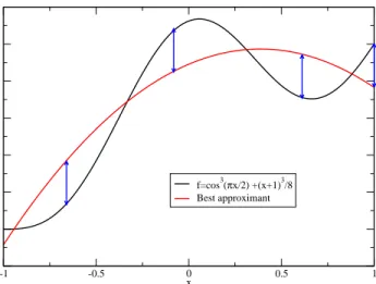
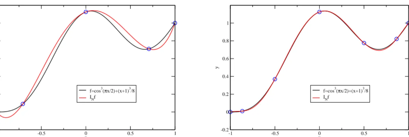
whereδ= 0 orδ= 1. An example of a function and its best polynomial approximation is shown of Fig. 1.

2.2

Interpolation on a Grid

AgridX on the interval [₋1,1] is a set ofN+ 1 pointsxi∈[−1,1], 0≤i≤N. Those points are

-1 -0.5 0 0.5 1 x -0.2 0 0.2 0.4 0.6 0.8 1 y f=cos3(πx/2) +(x+1)3/8 Best approximant N=2

Figure 1: Functionf = cos3_{(πx/2) + (x+ 1)}3_{/8(black curve) and its best approximation of degree}

2 (red curve). The blue arrows denote the4 points where the maximum error is attained.

Let us consider a continuous functionf and a gridX withN+ 1 nodesxi. Then, there exist

a unique polynomial of degreeN,IX

Nf, that coincides withf at each node :

INXf(xi) =f(xi) 0≤i≤N. (19)

IX

Nf is called the interpolant off through the gridX. INXf can be expressed in terms of the

Lagrange cardinal polynomials:

IX Nf = N X i=0 f(xi)lXi (x), (20) where the lX

i are the Lagrange cardinal polynomials. By definition, liX is the unique polynomial

of degree N, that vanishes at all nodes of the grid X butat xi, where it is 1. It is easy to show

that the Lagrange cardinal polynomials can be written as

lXi (x) = N Y j=0,j6=i x₋xj xi−xj . (21)

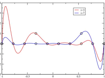
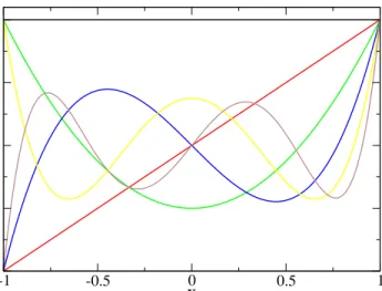
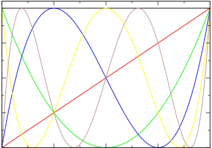
Figure 2 shows some examples of Lagrange cardinal polynomials and an example of a function and its interpolant on a uniform grid can be seen on Fig. 3.

Thanks to Chebyshev alternate theorem, one can see that the best approximation of degreeN

is an interpolant of the function atN+ 1 nodes. However, in general, the associated grid is not known. The difference between the error made by interpolating on a given gridX can be compared to the smallest possible error for the best approximation. One can show that :

f −I_NXf

-1 -0.5 0 0.5 1 x -3 -2 -1 0 1 2 3 4 y i=3 i=7 Uniform grid N=8

Figure 2: Lagrange cardinal polynomials lX

3 (red curve) and lX7 on an uniform grid with N = 8.

The black circles denote the nodes of the grid.

-1 -0.5 0 0.5 1 x -0.2 0 0.2 0.4 0.6 0.8 1 y f=cos3(πx/2)+(x+1)3/8 Interpolant (uniform grid)

N=4

Figure 3: Functionf = cos3_{(πx/2) + (x+ 1)}3

/8(black curve) and its interpolant (red curve)on a

-1 -0.5 0 0.5 1 x -0.5 0 0.5 1 y f = 1/(1+16x2) Uniform interpolant N=4 -1 -0.5 0 0.5 1 x -0.5 0 0.5 1 y f=1/(1+16x2) Uniform interpolant N=13 Figure 4: Function f = 1

1 + 16x2 (black curve) and its interpolant (red curve)on a uniform grid

of5 nodes (left panel) and14 nodes (right panel). The blue circles show the position of the nodes.

where Λ is theLebesgue constantof the gridX and is defined as :

ΛN(X) = maxx∈[−1,1] N X

i=0

|lxi (x)|. (23)

A theorem by Erd¨os (1961) states that, for any choice of gridX, there exist a constantC >0 such that :

ΛN(X)> 2

πln (N+ 1)−C. (24)

It immediately follows that Λ (N)→ ∞whenN → ∞. This implies that for any grid, there always exists at least one continuous functionf which interpolant does not converge uniformly tof. An example of such failure of the convergence is show on Fig. 4, where the interpolant of the function

f = 11 + 16x2 is clearly not uniform (see the behavior near the boundaries of the interval). This is known as the Runge phenomenon.

Moreover, a theorem by Cauchy states that, for all functions f _{∈ C}(N+1)_{, the interpolation}

error, on a gridX ofN+ 1 nodes is given by

f(x)₋INX(x) = fN+1_(ǫ) (N+ 1)!w X N+1(x), (25) whereǫ_∈[₋1,1]. wX

N+1 is the nodal polynomial ofX, being the only polynomial of degreeN+ 1,

with a leading coefficient 1 and that vanishes on the nodes ofX. It is then easy to show that

wX N+1(x) = N Y i=0 (x₋xi). (26)

On equation (25), one has a priori no control on the term involvingfN+1_{. For a given function,}

this can be rather large and this is indeed the case for the functionf shown on Fig. 4. However, one can hope to minimize the interpolation error by choosing a grid such that the nodal polynomial

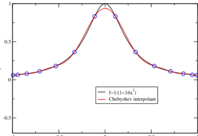
-1 -0.5 0 0.5 1 x -0.5 0 0.5 1 y f = 1/(1+16x2) Chebyshev interpolant N=4 -1 -0.5 0 0.5 1 x -0.5 0 0.5 1 y f=1/(1+16x2) Chebyshev interpolant N=13

Figure 5: Same thing as Fig. 4 but using a grid based on the zeros of Chebyshev polynomials. The Runge phenomenon is no longer present.

is as small as possible. A theorem by Chebyshev states that this choice is unique and is given by a grid which nodes are the zeros of the Chebyshev polynomialTN+1(see Sec. 2.3 for more details

on Chebyshev polynomials). With such a grid, one can achieve

w_NX₊₁ ∞= 1 2N, (27)

which is the smallest possible value. So, a grid based on nodes of Chebyshev polynomials can be expected to perform better that a standard uniform one. This is what can be seen on Fig. 5, which shows the same thing than Fig. 4 but with a Chebyshev grid. Clearly, the Runge phenomenon is no longer present. It can be checked, that, for this choice of functionf, the uniform convergence of the interpolant to the function is recovered.

2.3

Polynomial Interpolation

2.3.1 Orthogonal polynomials

Spectral methods are based on the notion oforthogonal polynomials. In order to define orthogo-nality, one has to define the scalar product of two functions, on an interval [₋1,1]. Let us consider a positive functionwof [₋1,1] called themeasure. The scalar product off andg, with respect to this measure is defined as :

(f, g)_w=

Z

x∈[−1,1]

f(x)g(x)w(x) dx. (28)

A basis of PN is then a set of N + 1 polynomials pn, each of degree n that are orthogonal :

(pi, pj)_w= 0 fori6=j.

The projectionPNf of a functionf on this basis is then

PNf = N X n=0 ˆ fnpn, (29)

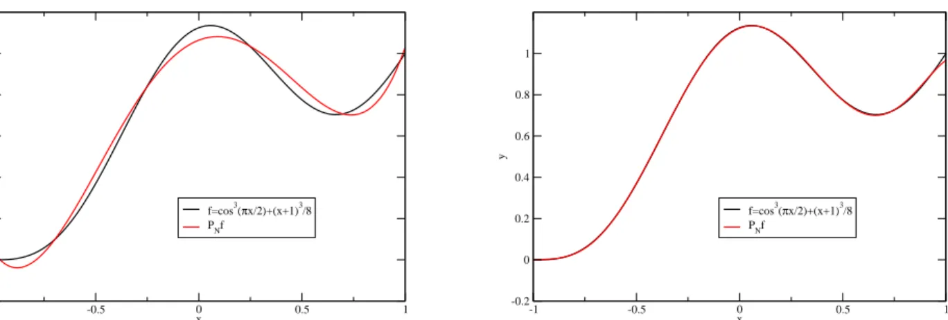
-1 -0.5 0 0.5 1 x -0.2 0 0.2 0.4 0.6 0.8 1 y f=cos3(πx/2)+(x+1)3/8 P_Nf N=4 -1 -0.5 0 0.5 1 x -0.2 0 0.2 0.4 0.6 0.8 1 y f=cos3(πx/2)+(x+1)3/8 P_Nf N=8

Figure 6: Function f = cos3_{(πx/2) + (x+ 1)}3

/8 (black curve) and its projection on Chebyshev

polynomials (red curve), for N = 4(left panel) and N = 8(right panel).

where the coefficients of the projection are given by ˆ

fn=

(f, pn)

(pn, pn)

. (30)

The difference betweenf and its projection goes to zero whenN increases :

kf ₋PNfk∞→0 when N → ∞. (31)

Figure 6 shows the functionf = cos3_{(πx/2) + (x+ 1)}3

/8 and its projection on Chebyshev poly-nomials (see Sec. 2.4.2), for N = 4 and N = 8, illustrating the rapid convergence of PNf to

f.

At first sight, the projection seems to be an interesting mean of numerically representing a function. However, in practice, this is not the case. Indeed, to determine the projection of a function, one needs to compute the integrals (30), which requires the evaluation of f at a great number of points, thus making the all numerical scheme impracticable.

2.3.2 Gaussian quadratures

The main theorem of Gaussian quadratures states that, given a measure w, there exist N + 1 positive realswn andN+ 1 realsxn∈[−1,1] such that:

∀f ∈P_2N+δ, Z [−1,1] f(x)w(x) dx= N X n=0 f(xn)wn. (32)

Thewnare called theweightsand thexn are the collocation points. The degree of applicability of

the theorem depends on the integerδ, which can take the following values.

• Gauss quadrature : δ= 1.

• Gauss-Lobatto : δ=−1 andx0=−1 andxN = 1.

Gauss quadrature is more appealing because it applies to polynomials of higher degree but Gauss-Lobatto quadrature is often more useful for numerical purposes because the outermost collocation points coincide with the boundaries of the interval making is easier to impose continuities or boundary conditions.

2.3.3 Spectral interpolation

As already stated in 2.3.1, the main shortcoming of projecting a function on orthogonal polyno-mials comes from the difficulty to compute the integrals (30). The idea of spectral methods is to approximate the coefficients of the projection by making use of the Gaussian quadratures. By doing so, one can define theinterpolantof a functionf by

INf = N X n=0 ˜ fnpn(x), (33) where ˜ fn= 1 γn N X i=0 f(xi)pn(xj)wi and γn = N X i=0 p2n(xi)wi. (34)

The ˜fn exactly coincides with the coefficients ˆfn, if the Gaussian quadrature is applicable for

computing (30), that is for allf ∈P_{N+δ. So, in general, INf 6=PNf and the difference between} the two is called the aliasing error. The advantage of using the ˜f is that they are computed by estimatingf at theN+ 1 collocation points only.

One can show that INf and f coincide at the collocation points : INf(xi) = f(xi) so that

IN interpolatesf on the grid which nodes are the collocation points. Figure 7 shows the function

f = cos3_{(πx/2)+(x+ 1)}3

/8 and its spectral interpolation using Chebyshev polynomials, forN= 4 andN = 6.

2.3.4 Two equivalent descriptions

The description of a functionf in terms of its spectral interpolation can be given in two different but equivalent spaces:

• in the configuration space if the function is described by its value at the N+ 1 collocation pointsf(xi).

• in the coefficient space if one works with theN+ 1 coefficients ˜fi.

There is a bijection between the two spaces and the following relations enable to go from one description to the other:

• the coefficients can be computed from the values off(xi) using Eq. (34).

• the values at the collocation points are expressed in terms of the coefficients by making use of the definition of the interpolant (33):

f(xi) = N X n=0 ˜ fnpn(xi). (35)

-1 -0.5 0 0.5 1 x -0.2 0 0.2 0.4 0.6 0.8 1 y f=cos3(πx/2)+(x+1)3/8 I_Nf N=4 -1 -0.5 0 0.5 1 x -0.2 0 0.2 0.4 0.6 0.8 1 y f=cos3(πx/2)+(x+1)3/8 I_Nf N=6

Figure 7: Functionf = cos3_{(πx/2) + (x+ 1)}3

/8(black curve) and its interpolant INf Chebyshev

polynomials (red curve), for N = 4 (left panel) and N = 6(right panel). The collocation points

are denoted by the blue circles and correspond to Gauss-Lobatto quadrature.

Depending on the operation one has to perform on a given function, it may be more clever to work in one space or the other. For instance, the square root of a function is very easily given in the collocation space by √f(xi), whereas the derivative can be computed in the coefficient

space, if, and this is generally the case, the derivatives of the basis polynomials are known, by

f′₌ N X n=0 ˜ fnp′n(x).

2.4

Usual polynomials

In this section, some commonly used sets of orthogonal functions are presented.

2.4.1 Legendre polynomials

Legendre polynomialsPn are orthogonal on [−1,1] with respect to the measurew(x) = 1.

More-over, the scalar product of two polynomials is given by : (Pn, Pm) = Z 1 −1 PnPmdx= 2 2n+ 1δmn. (36)

Starting fromP0= 1 andP1=x, the successive polynomials can be computed by the following

recurrence expression:

(n+ 1)Pn+1(x) = (2n+ 1)xPn(x)−nPn−1(x). (37)

Amongst the various properties of Legendre polynomials, one can note that i)Pn has the same

parity asn. ii)Pn is of degreen. iii)Pn(±1) = (−1)n. iv)Pn has exactlynzeros on [−1,1]. The

first polynomials are shown on Fig. 8.

The weights and location of the collocation points associated with Legendre polynomials depend on the choice of quadrature.

-1 -0.5 0 0.5 1

x

Figure 8: First Legendre polynomials, from P0 toP5.

• Legendre-Gauss : xi are the nodes ofPN+1 andwi =

2 (1₋x2 i) P′ N+1(xi) 2.

• Legendre-Gauss-Radau : x0=−1 and the xi are the nodes ofPN+PN+1. The weights are

given byw0=

2

(N+ 1)2 andwi = 1 (N+ 1)2.

• Legendre-Gauss-Lobatto : x0=−1,xN =−1 andxi are the nodes ofPN′ . The weights are

wi= 2

N(N+ 1) 1 [PN(xi)]2

.

Those values are not analytic but can be computed numerically in an efficient way.

Some elementary operations can be easily performed on the coefficient space. Let us assume that a functionf is given by its coefficientsan so thatf =

N X

n=0

anPn. Then the coefficientsbn of

Hf =

N X

n=0

bnPn can be found as a function of thean, for various operatorsH. For instance,

• ifH is the multiplication byxthen :

bn= n 2n₋1an−1+ n+ 1 2n+ 3an+1 (n≥1). (38) • ifH is the derivation : bn= (2n+ 1) N X p=n+1,p+nodd ap. (39)

-1 -0.5 0 0.5 1 x -1 -0.5 0 0.5 1

Figure 9: First Chebyshev polynomials, fromT0 toT5.

• ifH is the second derivation :

bn= (n+ 1/2)

N X

p=n+2,p+neven

[p(p+ 1)₋n(n+ 1)]ap. (40)

Those kind of relations enable to represent the action ofH as a matrix acting on the vector of the

an, the product being the coefficients ofHf, i.e. the bn.

2.4.2 Chebyshev polynomials

Chebyshev polynomials, denoted by Tn, are orthogonal on [−1,1] with respect to the measure

w= 1/√1₋x2 _{and the scalar product of two polynomials is}

(Tn, Tm) = Z 1 −1 TnTm √ 1−x2dx= π 2(1 +δ0n)δmn. (41) Given thatT0= 1 andT1=x, the higher order polynomials can be obtained by making use of the

recurrence

Tn+1(x) = 2xTn(x)−Tn−1(x). (42)

This implies the following simple properties. i)Tn has the same parity asn. ii)Tn is of degreen.

iii) Tn(±1) = (−1)n. iv) Tn has exactly n zeros on [−1,1]. The first polynomials are shown on

Fig. 9.

Contrary to the Legendre case, both the weights and position of the collocation points are analytical and given by :

• Chebyshev-Gauss : xi= cos

(2i+ 1)π

2N+ 2 and wi=

π N+ 1.

• Chebyshev-Gauss-Radau :xi= cos 2πi

2N+ 1. The weights arew0=

π 2N+ 1andwi= 2π 2N+ 1 • Chebyshev-Gauss-Lobatto : xi= cos πi

N. The weights arew0=wN = π

2N andwi= π N.

As for the Legendre case, the action of various linear operators H can be expressed in the coefficient space. This means that the coefficientsbnofHf are given as functions of the coefficients

an off. For instance,

• ifH is the multiplication byxthen :

bn =1 2[(1 +δ0n−1)an−1+an+1] (n≥1). (43) • ifH is the derivation : bn= 2 (1 +δ0n) N X p=n+1,p+nodd pap. (44)

• ifH is the second derivation :

bn= 1 (1 +δ0n) N X p=n+2,p+neven p p2₋n2 ap. (45) 2.4.3 Convergence properties

One of the main advantage of spectral method is the very fast convergence of the interpolantINf

to the function f, at least for smooth enough functions. Let us consider a _Cm _{function u, then,}

one can place the following upper bounds on the difference betweenuand its interpolantINu:

• For Legendre : kINu−uk_L2 ≤ C1 Nm−1/2 m X k=0 u (k) _L2. (46) • For Chebyshev : kINu−uk_L2 w ≤ C2 Nm m X k=0 u (k) L2 w . (47) kINu−uk_∞≤ C3 Nm−1/2 m X k=0 u (k) L2 w . (48)

The Ci are some positive constants. An interesting limit of the above estimates concerns a C∞

function. One can then see that the difference between uandINudecays faster than any power

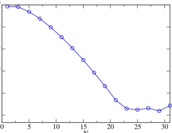
of N. It implies that the error decays exponentially and one talks about an evanescent error. An example of this very fast convergence is shown on Fig. 10. The error clearly decays as an exponential, until the level of 10−14_{of the precision of the computation is reached (one is working}

in double precision in this particular case). Fig. 10 illustrates the fact that, with spectral methods, very good accuracy can be reached with only a moderate number of coefficients.

If the function is less regular (i.e. not_C∞_{), the error is no longer exponential and only decays}

as a power-law, thus making the use of spectral method less appealing. This effect is called the Gibbs phenomenon. It can be easily seen on the worst possible case, the one of a discontinuous function (m = 0). In the case, the estimates (46-48) do not even ensure convergence at all. On Fig. 11 one shows a step function and its interpolant, for various values of N. One can see that the maximum difference between the function and its interpolant is not even going to zero when

0 5 10 15 20 25 30 N 10-15 10-12 10-9 10-6 10-3 100 max Λ |I N f -f|

Figure 10: Maximum difference betweenf = cos3_{(πx/2) + (x+ 1)}3

/8 and its interpolant INf, as

a function ofN. -1 -0.8 -0.6 -0.4 -0.2 0 0.2 0.4 0.6 0.8 1 x -0.2 0 0.2 0.4 0.6 0.8 1 N = 5N = 9 N = 17

2.4.4 Trigonometrical functions

A detailed presentation of the theory of Fourier transform is beyond the scope of this work. How-ever, there is a close link between the so-calleddiscrete Fourier transform and the spectral inter-polation and this is briefly outlined here.

The Fourier transformP f of a functionf of [0,2π] is given by :

P f(x) =a0+ ∞ X n=1 ancos (nx) + ∞ X n=1 bnsin (nx). (49)

The Fourier transform is known to converge rather rapidly to the function itself. However, the coef-ficientsan andbn are given by integrals like

Z 2π

0

f(x) cos (nx) dxthat can not be easily computed (as it was the case for the projection of a function on orthogonal polynomials in Sec. 2.3.1).

The solution to this problem is also very similar to the use of the Gaussian quadratures. Let us introduceN + 1 collocation pointsxi = 2πi/(N+ 1). Then, the discrete Fourier coefficients

with respect to those points are : ˜ a0 = 1 N N X k=1 f(xk) (50) ˜ an = 2 N N X k=1 f(xk) cos (nxk) (51) ˜_{bn =} 2 N N X k=1 f(xk) sin (nxk) (52)

and the interpolantINf is then given by :

INf(x) = ˜a0+ N X n=1 ˜ ancos (nx) + N X n=1 ˜ bnsin (nx). (53)

The approximation made by using the discrete coefficients in place of the real ones is of the same nature than the one made when computing the coefficients of the projection (30) by means of the Gaussian quadratures. Let us mention that, in the case of a discrete Fourier transform, the first and last collocation points lies on the boundary of the interval, as for a Gauss-Lobatto quadrature. As for the polynomial interpolation, the convergence ofINf to f is exponential, for

all periodic and_C∞_functions.

2.4.5 Choice of basis

For periodic functions of [0,2π[, the discrete Fourier transform is the natural choice of basis. If the considered function has also some symmetries, one can use a subset of the trigonometrical polynomials. For instance, if the function is i) periodic on [0, ,2π[ and is also odd with respect to

x=π, then it can be expanded on sines only.

If the function is not periodic, then it is natural to expand it either on Chebyshev or Legendre polynomials. Chebyshev polynomials have two main advantages. First the associated weights and collocation points are analytical and second, the coefficients can be computed by means of FFT algorithms. The use of an FFT reduces the number of operations fromN2_{when using the standard}

formula Eq. (34) to onlyNlnN operations. For codes where most of the computational time is spent going from one representation space to the other, this may be an interesting feature. The

main advantage of Legendre polynomials is the fact that the associated measure is very simple

w(x) = 1. The multi-domain technique presented in Sec. 2.6.4 is one particular example where such property is required.

2.5

Spectral Methods for ODEs

2.5.1 Weighted residual method

Let us consider a differential equation of the following form

Lu(x) =S(x), x∈[−1,1], (54) where L is a linear, second order, differential operator. The problem admits a unique solution once some boundary conditions are prescribed atx= 1 and x=₋1. Typically, one can specify i) the value ofu (Dirichlet-type) ii) the value of its derivative ∂xu(Neumann-type) iii) a linear

combination of the two (Robin-type).

As for the elementary operations presented in Sec. 2.4.1 and 2.4.2, the action ofLonucan be expressed by a matrixLij. If the coefficients ofuwith respect to a given basis are the ˜ui, then the

coefficients ofLuare

N X

j=0

Lij˜uj. (55)

TheLijcan usually be easily computed by combining the action of elementary operations like the

second derivation, the first derivation, the multiplication or division byx(see Sec. 2.4.1 and 2.4.2 for some examples).

A function uis an admissible solution of the problem if and only if i) it fulfills the boundary conditions exactly (up to machine accuracy) ii) it makes the residual R =Lu₋S small. In the weighted residual method, one considers a set ofN+ 1 test functionsξn on [−1,1]. The smallness

ofRis enforced by demanding that

(R, ξk) = 0,∀k≤N. (56)

AsN increases, the obtained solution is closer and closer to the real one. Depending on the choice of the test functions and the way the boundary conditions are enforced, one gets various solvers. Three classical examples are presented next.

2.5.2 The Tau-method

In this particular method, the test functions coincide with the basis used for the spectral expansion, for instance the Chebyshev polynomials. Let us denote ˜ui and ˜si the coefficients of the solutionu

and the sourceS with respect to Chebyshev polynomials.

Given the expression ofLuin the coefficient space (55) and the fact that the basis polynomials are orthogonal, the residual equations (56) are expressed as

N X

i=0

Lniu˜i= ˜sn, ∀n≤N, (57)

the unknowns being the ˜ui. However, as such, this system does not admit a unique solution, due

to the homogeneous solutions ofL (i.e. the matrix associated with L is not invertible) and one has to impose the boundary conditions. In the Tau-method, this is done by relaxing thelast two

equations (57) (i.e. forn=N₋1 andn=N) and by replacing them by the boundary conditions atx=₋1 andx= 1.

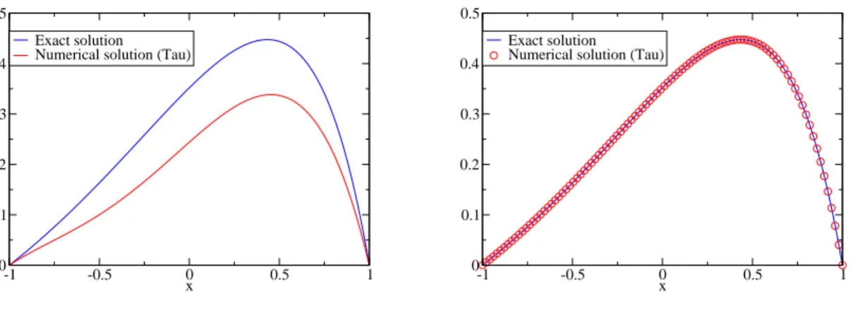
-1 -0.5 0 0.5 1 x 0 0.1 0.2 0.3 0.4 0.5 Exact solution Numerical solution (Tau)

N=4 -1 -0.5 0 0.5 1 x 0 0.1 0.2 0.3 0.4 0.5 Exact solution Numerical solution (Tau)

N=8

Figure 12: Exact solution (60) of Eq. (58) (blue curve) and the numerical solution (red curves)

computed by means of a Tau-method, forN = 4(left panel) andN = 8(right panel).

The Tau-method thus ensures thatLuandShave the same coefficients but for the last ones. If the functions are smooth, then their coefficients should decrease exponentially (evanescent error) and so the “forgotten” conditions are less and less stringent whenN increases, ensuring that the computed solution converges rapidly to the real one.

As an illustration, let us consider the following equation : d2_u dx2−4 du dx+ 4u= exp (x)− 4e (1 +x2₎ (58)

with the following boundary conditions

u(x=₋1) = 0 andu(x= 1) = 0. (59) The solution exact is analytical and is

u(x) = exp (x)₋sinh (1)

sinh (2)exp (2x)−

e

(1 +x2₎. (60)

Fig. 12 shows the exact solution and the numerical one, for two different values of N. One can note that the numerical solution converges rapidly to the numerical one, the two being almost indistinguishable for N as small as N = 8. The numerical solution exactly fulfills the boundary conditions, no matter whatN is.

2.5.3 The collocation method

The collocation method is very similar to the Tau-method. They only differ from the choice of test functions. Indeed, in the collocation method one uses continuous function that are zero at each but one collocation point. They are indeed the Lagrange cardinal polynomials already seen in Sec. 2.2 and can be written asξi(xj) =δij. With such test functions, the residual equations (56) are

Lu(xn) =S(xn), ∀n≤N. (61)

The value ofLuat each collocation points is easily expressed in terms of the ˜uby making use of (55) and one gets :

N X i=0 N X j=0 Liju˜jTi(xn) =S(xn), ∀n≤N. (62)

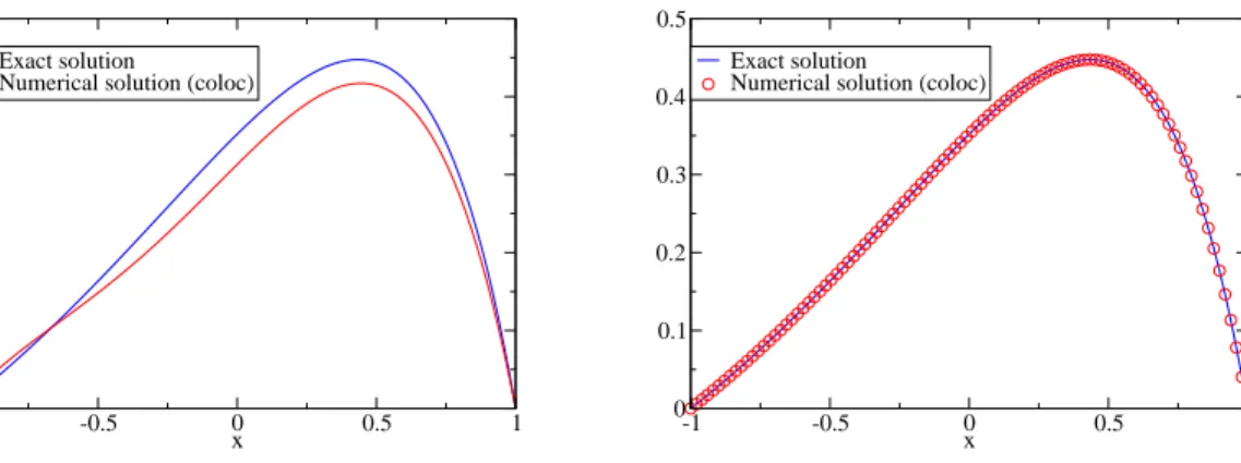
-1 -0.5 0 0.5 1 x 0 0.1 0.2 0.3 0.4 0.5 Exact solution

Numerical solution (coloc) N=4 -1 -0.5 0 0.5 1 x 0 0.1 0.2 0.3 0.4 0.5 Exact solution

Numerical solution (coloc) N=8

Figure 13: Same as Fig. 12 but for the collocation method.

Let us note that, even if the collocation method imposes that Lu and S coincide at each collocation point, the unknowns of the system written in the form (62) are the coefficients ˜unand

not theu(xn). As for the Tau-method, the system (62) is not invertible and boundary conditions

must be enforced by additional equations. In this case, the relaxed conditions are the two associated with the outermost points, i.e. n= 0 and n =N, which are replaced by appropriate boundary conditions to get an invertible system.

Fig. 13 shows both the exact and numerical solutions for Eq. (58).

2.5.4 Galerkin method

The basic idea of Galerkin method is to seek the solution u as a sum of polynomials Gi that

individuallyverify the boundary conditions. Doing souautomatically fulfills those conditions and

they do not have to be imposed by additional equations. Such polynomials constitute a Galerkin basis of the problem. For practical reasons, it is better to chose a Galerkin basis that can be expressed easily in terms of the original orthogonal polynomials.

For instance, with the boundary conditions (59), one can choose :

G2k(x) = T2k+2(x)−T0(x) (63)

G2k+1(x) = T2k+3(x)−T1(x) (64)

More generally, the Galerkin basis relates to the usual ones by means of a transformation matrix

Gi= N X

j=0

MjiTj, ∀i≤N−2. (65)

Let us mention that the matrixM is not square. Indeed, to maintain the same degree of approx-imation, one can consider onlyN−1 Galerkin polynomials, due to the two additional conditions they have to fulfill (see for instance Eqs. (63-64)). One can also note that, in general, theGi are

notorthogonal polynomials.

The solutionuis sought in terms of the coefficients ˜uG

i on the Galerkin basis :

u(x) = N−2 X k=0 ˜ uGkGk(x). (66)

-1 -0.5 0 0.5 1 x 0 0.1 0.2 0.3 0.4 0.5 Exact solution

Numerical solution (Galerkin) N=4 -1 -0.5 0 0.5 1 x 0 0.1 0.2 0.3 0.4 0.5 Exact solution

Numerical solution (Galerkin) N=8

Figure 14: Same as Fig. 12 but for the Galerkin method.

By making use of Eqs. (55) and (65) one can expressLuin terms of the ˜uG i : Lu(x) = N−2 X k=0 ˜ uGk N X i=0 N X j=0 MjkLijTi(x). (67)

The test functions used in the Galerkin method are the Gi themselves so that the residual

system reads :

(Lu, Gn) = (S, Gn), ∀n≤N−2 (68)

where the left-hand-side is computed by means of (67) and by expressing theGi in terms of theTi

by (65). Concerning the right-hand-side, the source itself is notexpanded on the Galerkin basis, given that it does not fulfill the boundary conditions. Putting all the pieces together, the Galerkin system reads : N−2 X k=0 ˜ uG k N X i=0 N X j=0 MinMjkLij(Ti|Ti) = N X i=0 Mins˜i(Ti|Ti), ∀n≤N−2. (69)

This is a system of N₋1 equations for the N ₋1 unknowns ˜uG

i and it can be directly solved,

being well-posed. Once the ˜uG

i are known, one can obtain the solution in terms of the usual basis

by making, once again, use of the transformation matrix :

u(x) = N X i=0 N−2 X n=0 Min˜uGn ! Ti. (70)

The solution obtained by the application of this method to the equation (58) is shown on Fig. 14.

2.5.5 The methods are optimal

A numerical method is said to be optimal if it does not introduce an additional error to the one that would be done by interpolating the exact solution of a given equation.

Let us calluexactsuch exact solution, unknown in general. Its interpolant is INuexact and the

numerical solution of the equation isunum. The numerical method is then optimal if and only if kINuexact−uexactk∞andkunum−uexactk∞ behave in the same manner whenN → ∞.

5 10 15 20 25 N 10-16 10-14 10-12 10-10 10-8 10-6 10-4 10-2 Error Tau Collocation Galerkin Interpolation

Figure 15: Difference between the exact solution (60) of Eq. (58)and its interpolant (black curve) and between the exact and numerical solutions for i) the tau method (green curve and circle symbols) ii) the collocation method (blue curve and square symbols) iii) the Galerkin method (red curve and triangle symbols).

In general, optimality is difficult to check because bothuexactand its interpolant are unknown.

However, for the test problem proposed in Sec. 2.5.2 this can be done. Fig. 15 shows the maximum relative difference between the exact solution (60) and its interpolant and the various numerical solutions. All the curves behave in the same manner as N increases, indicating that the three methods previously presented are optimal (at least for this particular case).

2.6

Multi-domain Techniques

2.6.1 Motivations and setting

A seen in Sec. 2.4.3, spectral methods are very efficient when dealing withC∞_{functions. However,}

they lose some of their appeal when dealing with less regular functions, the convergence to the exact functions being substantially slower. Nevertheless, at times, the physicist has to deal with such fields. This is the case for the density jump at the surface of strange stars or the formation of shocks to mention only two examples.

In order to maintain spectral convergence, one then needs to introduce several computational domains such that the various discontinuities of the functions lie at the interface between the domains. Doing so,in each domain, one only deals with_C∞_functions.

In the following, three different multi-domain methods are presented to solve an equation of the type Lu =S on [₋1,1]. L is a second order linear operator and S a given source function. Appropriate boundary conditions are given at the boundariesx=₋1 andx= 1.

For simplicity the physical space is split into two domains:

• first domain : x≤0 described by x1= 2x+ 1, x1∈[−1,1], • second domain : x≥0 described byx2= 2x−1, x2∈[−1,1].

Ifx_≤0, a functionuis described by its interpolant in terms ofx1: INu(x) = N X i=0 ˜ u1iTi(x1(x)). The

same thing is true forx_≥0 with respect to the variablex2. Such setting is obviously appropriate

to deal with problems where discontinuities occur atx= 0, that isx1= 1 andx2=−1.

2.6.2 Multi-domain tau method

As for the standard tau-method (see Sec. 2.5.2) and in each domain, the test functions are the basis polynomials and one writes the associated residual equations. For instance in the domain

x_≤0 one gets: (Tn, R) = 0 =⇒ N X i=0 Lni˜u1i = ˜s1n ∀n≤N, (71)

the ˜s1 _{being the coefficients of the source and L}

ij the matrix representation of the operator. As

for the one-domain case, one relaxes the last two equations, keeping only N−1 equations. The same thing is done in the second domain.

Two supplementary equations are enforced to ensure that the boundary conditions are fulfilled. Finally, the operator Lbeing of second order, one needs to ensure that the solution andits first derivative are continuous at the interfacex= 0. This translates as a set of two additional equations involving the coefficients in both domains.

So, one considers

• N₋1 residual equations in the first domain,

• N−1 residual equations in the second domain,

• 2 boundary conditions,

• 2 matching conditions,

for a total of 2N+ 2 equations. The unknowns are the coefficients ofuin both domains (i.e. the ˜

u1i and the ˜u2i), that is 2N+ 2 unknowns. The system is well posed and admits a unique solution.

2.6.3 Method based on the homogeneous solutions

The method exposed here proceeds in two steps. First, particular solutions are computed in each domain. Then, appropriate linear combination with the homogeneous solutions of the operatorL

are performed to ensure continuity and impose boundary conditions.

In order to compute particular solutions, one can rely on any of the methods exposed in Sec. 2.5. The boundary conditions at the boundary of each domain can be chosen to be (almost) anything. For instance one can use, in each domain, a collocation method to solveLu=S, demanding that the particular solutionupartis zero at both end of each intervals.

Then, in order to have a solution in the whole space, one needs to add homogeneous solutions to the particular ones. In general, the operatorLis of second order and it admits two independent homogeneous solutions g and h, in each domain. Let us note that, in some cases, additional regularity conditions can reduce the number of available homogeneous solutions. The homogeneous solutions can either be computed analytically if the operatorL is simple enough or numerically but one then needs to have a method for solvingLu= 0.

In each domain, the physical solution is a combination of the particular solution and the homogeneous ones of the type :

whereαandβ are constants that must be determined. In the two domains case, we are left with 4 unknowns. The system they must verify is composed of i) 2 equations for the boundary conditions ii) 2 equations for the matching of u and its first derivative across the boundary between the two domains. The obtained system is called the matching system and generally admits a unique solution.

2.6.4 Variational method

Contrary to the methods previously presented, the variational one is only applicable with Legendre polynomials. Indeed, the methods requires that the measure isw(x) = 1. It is also useful to extract the second order term of the operatorLand to rewrite it likeLu=u′′_{+H,H being of first order}

only.

In each domain, one writes the residual equation explicitly : (ξ, R) = 0 =_⇒ Z ξu′′dx+ Z ξ(Hu) dx= Z ξSdx. (73)

The term involving the second derivative ofuis then integrated by parts :

[ξu′]₋ Z ξ′u′dx+ Z ξ(Hu) dx= Z ξSdx. (74)

The test functions are the same as the ones used for the collocation method, i.e. functions being zero at all but one collocation point: ξi(xj) =δij. By making use of the Gauss quadratures,

the various parts of Eq. (74) can then be expressed as:

Z ξ′nu′dx = N X i=0 ξn′ (xi)u′(xi)wi= N X i=0 N X j=0 DijDinwiu(xj) (75) Z ξn(Hu) dx = N X i=0 ξn(xi) (Hu) (xi)wi=wn N X i=0 Hniu(xi) (76) Z ξnSdx = N X i=0 ξn(xi)S(xi)wi=S(xn)wn, (77)

whereDij (resp. Hij) represent the action of the derivative (resp. ofH)in the configuration space

g′(xk) = N X j=0 Dkjg(xj) (78) (Hg) (xk) = N X j=0 Hkjg(xj). (79)

For points strictlyinside each domain, the integrated term [ξu′_{] of Eq. (74) vanishes and one}

gets equations like:

− N X i=0 N X j=0 DijDinwiu(xj) +wn N X i=0 Hniu(xi) =S(xn)wn. (80)

This is a set ofN₋1 equations for each domains. In the above form, the unknowns are theu(xi),

As usual two additional equations are provided by appropriate boundary conditions at both end of the whole domain. One also gets an additional condition by matching the solution across the boundary between the two domains.

The last equation of the system is the matching of the first derivative of the solution. However, instead of writing it “explicitly”, this is done by making use of the integrated term in Eq. (74) and this is actually the crucial step of the whole method. Applying Eq. (74) to the last pointxN

of the first domain, one gets :

u′(x1= 1) = N X i=0 N X j=0 DijDiNwiu(xj)−wN N X i=0 HN iu(xi) +S(xN)wN. (81)

The same thing can be done with the first point of the second domain, to getu′_(x

2=−1) and the

last equation of the system is obtained by demanding thatu′_(x

1= 1) =u′(x2=−1) and relates

the values ofuin both domains.

Before finishing with the variational method, it may be worthwhile to explain why Legendre polynomials are used. Suppose one wants to work with Chebyshev polynomials instead . The measure is thenw(x) = √ 1

1₋x2. When one integrates the term containing u

′′ _{by part one then}

gets

Z

−u′′f wdx= [₋u′f w] +

Z

u′f′w′dx (82) Because the measure is divergent at the boundaries, it is difficult, if not impossible, to isolate the term inu′_{. On the other hand this is precisely the term that is needed to impose the appropriate}

matching of the solution.

2.6.5 Merits of the various methods

From a numerical point of view, the method based on an explicit matching using the homogeneous solutions is somewhat different from the two others. Indeed, one has to solve several systems in a row but each one is of the same size than the number of points in one domain. On the contrary, for both the variational and the tau method one has to solve only one system but its size is the same as the number of points in whole space, which can be quite big for settings with many domains. However, those two methods do not require to compute the homogeneous solutions, computation that could be tricky depending on the operators involved and on the number of dimensions. It is also true that the Tau-method is somewhat more difficult to generalized to the higher-dimensional case than the collocation method.

The variational method may seem more difficult to implement and is only applicable with Legendre polynomials, prohibiting the use of any FFT algorithms to compute the coefficients. However, on the mathematical grounds, it is the only method which is demonstrated to be optimal. Moreover, some examples have been found where the others methods are not optimal.

The choice of one method or another thus depend on the particularity of the situation. As for the mono-domain space, for simple tests problems, the results are very similar. Fig. 16 shows the maximum error between the analytical solution and the numerical one for the three different methods. All errors are evanescent and reach machine accuracy with the roughly same number of points.

5 10 15 20 25 30 35 N 10-16 10-14 10-12 10-10 10-8 10-6 10-4 10-2 Error Tau method Homogeneous Variational

Figure 16: Difference between the exact and numerical solutions of the following test problem.

d2_u

dx2+ 4u=S, withS(x <0) = 1andS(x >0) = 0. The boundary conditions areu(x=−1) = 0

andu(x= 1) = 0. The black curve and circles denote results from the multi-domain Tau method, the red curve and triangles from the method based on the homogeneous solutions and the blue curve and diamonds from the variational one.

3

Multi-dimensional cases: dealing with space and time

In principle, the generalization to more than one dimension is rather straightforward if one uses the tensorial product. Let us first take an example, with the spectral representation in terms of Chebyshev polynomials of a scalar functionf(x, y), defined on the square (x, y)_∈[₋1,1]_×[₋1,1]. One simply writes

f(x, y) = M X i=0 N X j=0 aijTi(x)Tj(y), (83)

withTi being the Chebyshev polynomial of degreei. The partial differential operators can also be

generalized, as being linear operators acting on the spaceP_M⊗P_{N. Simple, linear Partial} Differen-tial Equations (PDE) can be solved by one of the methods presented in Section 2.5 (Galerkin, tau or collocation), on thisM N-dimensional space. The development (83) can of course be generalized to any dimension. Some special PDE and spectral base examples, where the differential equation decouples for some of the coordinates, shall be given in Section 3.3. From a relativistic point of view, the time coordinate could be treated in this way and one should be able to achieve spec-tral accuracy for the time representation of a space-time function a(t, x, y, z) and its derivatives. Unfortunately, this does not seem to be the case and, we are not aware neither of any efficient algorithm for dealing with the time coordinate, nor of any published successful code solving any of the PDE coming from the Einstein equations.

3.1

Time Discretization

Why is time playing such a special role ? It is not obvious to find in the literature on spectral methods a complete and comprehensive study. A first standard explanation is the difficulty, in general, to predict the exact time interval on which one wants to study the time evolution. Then, time discretization errors in both finite-differences and spectral methods are typically much smaller than are spatial ones. Finally, one must keep in mind that, contrary to finite-differences, spectral methods are storing all global information about a function on the whole time interval. Therefore, a historical reason may be that, since until rather recently there were strong memory and CPU limitations to multi-dimensional simulations, it was not possible to (even hope to) describe a complete field depending on 3+1 coordinates. To this reason one can add the fact that, in the full 3+1 dimensional case, the matrix representing a differential operator would be of very big size; it would therefore be very time-consuming to invert it in a general case, even with iterative methods. Thus, there have been very few theoretical developments on the subject, with the exception of Ierley et al.[86], were the authors have applied spectral methods in time for the study of the Korteweg de Vries and Burger equations, using Fourier series in space and Chebyshev polynomials for the time coordinate. It is interesting to note that they observe a time-stepping restriction: they have to employ multi-domain and patching techniques (see Sec. 2.6) for the time interval, with the size of each sub-domain being roughly given by the Courant-Friedrichs-Lewy (CFL) condition. So the most common approach for time representation are finite-differences techniques, which allow for the use of many well-established time-marching schemes, and the method of lines (for other methods, including fractional stepping, see Fonrberg [61]).

3.1.1 Method of lines

Let us write the general form of a first-order in time linear PDE:

∂u

whereL is a linear operator containing only derivatives with respect to spatial coordinates. One can represent the function uthrough a finite setUN(t), composed of its time-dependent spectral

coefficients, or values at the collocation points. We note LN the spectral approximation to the

operatorL, together with the boundary conditions, if a tau or collocation method is used. LN is

therefore represented as anN_×N matrix. This is the so-called method of lines, which allows one to reduce a PDE to some ODE, after discretization in all dimensions but one. The advantage is that many ODE integration schemes are known (Runge-Kutta, symplectic integrators, ...) and can be used here. We shall suppose an equally-spaced grid in time, with the time-step noted ∆tand

UJ

N =UN(J×∆t). In order to step fromUNJ toU J+1

N , one has either to compute the action ofLN

on UN K

_K≤J (explicit schemes) or to solve for a boundary value problem in term ofU_NJ+1 (implicit

schemes). Both types of schemes have different stability properties, which can be analyzed as follows. Assuming thatLN can be diagonalized in the sense of the definition given in (3.1.3), the

stability study can be reduced to the study of the collection of scalar ODE problems

∂UN

∂t =λiUN, (85)

whereλi is any of the eigenvalues ofLN in the sense of Eq. (89).

3.1.2 Stability

The basic definition of stability for an ODE integration scheme is that, if the time-step is lower than some threshold, then _kUJ

Nk ≤ AeKJ∆t, with the constants A and K independent of the

time-step. This is perhaps not the most appropriate definition, since in practice one often deals with bounded functions and an exponential growth in time would not be acceptable. Therefore, an integration scheme is said to beabsolutely stable (or asymptotically stable), if kUJ

Nk remains

bounded,∀J ≥0. This property depends on a particular value of the product λi×∆t. For each

time integration scheme, theregion of absolute stability is the set of the complex plane containing all theλi∆t for which the scheme is absolutely stable.

Finally, a scheme is said to be A-stable if its region of absolute stability contains the half complex plane of numbers with negative real part. It is clear that no explicit scheme can be

A-stable due to the CFL condition. It has been shown by Dahlquist [51] that there is no linear multi-step method of order higher than 2 which isA-stable. Thus implicit methods are also limited in time-step size if more than second-order accurate. In addition, Dahlquist [51] shows that the most accurate second-orderA-stable scheme is the trapezoidal one (also called Crank-Nicolson, or second-order Adams-Moulton scheme)

U_NJ+1 =UNJ + ∆t 2 LNU J+1 N +LNU J N . (86)

On Figs. 17 and 18 are displayed the absolute stability regions for the Adams-Bashford and Runge-Kutta families of explicit schemes (see for instance [44]). For a given type of spatial linear operator, the requirement on the time-step usually comes from the largest (in modulus) eigenvalue of the operator. For example, in the case of the advection equation on [₋1,1], with a Dirichlet boundary condition

Lu=∂u

∂x,

u(1) = 0, (87)

and using a Chebyshev-tau method, one has that the largest eigenvalue ofLN grows in modulus

asN2_{. Therefore, for any of the schemes considered on Figs. 17-18, the time-step has a restriction}

of the type

-2 -1.5 -1 -0.5 0 0.5 1 Real part -1 -0.5 0 0.5 1 Imaginary part AB1 AB2 AB3 AB4

Figure 17: Regions of absolute stability for the Adams-Bashford integration schemes of order 1 to 4. -4 -3 -2 -1 0 1 2 3 4 Real part -4 -2 0 2 4 Imaginary part RK2 RK3 RK4 RK5

Figure 18: Regions of absolute stability for the Runge-Kutta integration schemes of order 2 to 5. Note that the size of the region is increasing with the order.

-200 -100 0 100 200 Real part -200 -100 0 100 200 Imaginary part N=17 N=33 N=65

Figure 19: Eigenvalues of the first derivative-tau operator (89) for Chebyshev polynomials. The largest (in modulus) eigenvalue is not displayed; this one is real, negative and goes asO(N2_).

which can be related to the usual CFL condition by the fact that the minimal distance between two points of a (N-point) Chebyshev grid decreases like O(N−2_{). Due to the above citedSecond}

Dahlquist barrier [51], implicit time marching schemes of order higher than two also have such

kind of limitation.

3.1.3 Spectrum of simple spatial operators

An important issue in determining the absolute stability of a time-marching scheme for the solution of a given PDE is the computation of the spectrum (λi) of the discretized spatial operatorLN (85).

As a matter of fact, these eigenvalues are those of the matrix representation ofLN, together with

the necessary boundary conditions for the problem to be well-posed (e.g. BNu= 0). If one notes

bthe number of such boundary conditions, each eigenvalueλi(here, in the case of the tau method)

is defined by the existence of a non-null set of coefficients{uj}_1≤j≤N such that

(_∀j) 1_≤j _≤N₋b, (LNu)j = λiuj,

BNu = 0. (89)

As an example, let us consider the case of the advection equation (first-order spatial derivative) with a Dirichlet boundary condition, solved with the Chebyshev-tau method (87). Because of the definition of the problem (89), there areN₋1 “eigenvalues”, which can be computed, after a small transformation, using any standard linear algebra package. For instance, it is possible, making use of the boundary condition, to express the last coefficient as a combination of the other ones

uN =− N−1

X

j=1

uj (90)

One is thus left with a usual eigenvalue problem for a (N ₋1)_×(N ₋1) matrix. Results are displayed on Figure 19 for three various values ofN. Real parts are all negative: the eigenvalue

which is not displayed lies on the negative part of the real axis and is much larger in modulus (it is growing likeO(N2_{)) than the N}

−1 others.

This way of determining the spectrum can be, of course, generalized to any linear spatial operator, for any spectral base, as well as to the collocation and Galerkin methods. Intuitively from CFL-type limitations, one can see that in the case of the heat equation (Lu = ∂2_u/∂x2_),

explicit time-integration schemes (or any scheme which is not A-stable) shall have a severe time-step limitation of the type

∆t.O(N4), (91)

for both Chebyshev or Legendre decomposition bases. Finally, one can decompose a higher-order in time PDE into a first-order system and then use one of the above proposed schemes. In the particular case of the wave equation

∂2_u

∂t2 =

∂2_u

∂x2, (92)

it is possible to write a second-order Crank-Nicolson scheme directly [110]

U_NJ+1= 2UNJ −UNJ−1+ ∆t2 2 ∂2UNJ+1 ∂x2 + ∂2UNJ−1 ∂x2 ! . (93)

Since this scheme isA-stable, there is no limitation on the time-step ∆t, but for explicit or higher-order schemes this limitation would be ∆t .O(N2_{), as for advection equation. The solution of}

such an implicit scheme is obtained as that of a boundary value problem at each time-step.

3.1.4 Semi-implicit schemes

It is sometimes possible to use a combination of implicit and explicit schemes to loosen a time-step restriction of the type (88). Let us consider as an example the advection equation with non-constant velocity on [₋1,1]

∂u ∂t =v(x)

∂u

∂x, (94)

with the relevant boundary conditions, which shall in general depend on the sign ofv(x). If on the one hand the stability condition for explicit time schemes (88) is too strong, and on the other hand an implicit scheme is too lengthy to implement or to use (because of the non-constant coefficient

v(x)), then it is interesting to consider the semi-implicit two-step method (see also [68])

U_NJ+1/2₋∆t 2 L − NU J+1/2 N = U J N + ∆t 2 LN −L − N UNJ, UNJ+1− ∆t 2 L + NUNJ+1 = U J+1/2 N + ∆t 2 LN−L + N UNJ+1/2, (95)

whereL+_NandL−_Nare respectively the spectral approximations to the constant operators−v(1)∂/∂x

and−v(−1)∂/∂x, together with the relevant boundary conditions (if any). This scheme is abso-lutely stable if

∆t. 1

Nmax_|v(x)_|. (96) With this type of scheme, the propagation of the wave at the boundary of the interval is treated implicitly, whereas the scheme is still explicit in the interior. The implementation of the implicit part, for which one needs to solve a boundary-value problem, is much easier than for the initial operator (94) because of the presence of only constant-coefficient operators. This technique is quite helpful in the case of more severe time-step restrictions (91), for example for a variable coefficient heat equation.