energies
ArticleRenewable Energy Sources and Battery Forecasting
Effects in Smart Power System Performance
Mehdi Bagheri1,* , Venera Nurmanova1, Oveis Abedinia2,3, Mohammad Salay Naderi4 , Noradin Ghadimi3,5and Mehdi Salay Naderi6
1 Department of Electrical and Computer Engineering, Nazarbayev University, Astana 010000, Kazakhstan;
2 Department of Electric Power Eng., Budapest University of Technology and Economics, Budapest 1111,
Hungary; [email protected]
3 Young Researchers and Elite Club, Islamic Azad University, Ardabil Branch, Ardabil 5615731567, Iran;
4 Electrical and Computer Engineering Department, Tehran North Branch, Islamic Azad University,
Tehran 1651153311, Iran; [email protected]
5 Department of Electrical engineering, Faculty of Technical Engineering, University of Mohaghegh Ardabili,
Ardabil 5615731567, Iran
6 Iran Grid Secure Operation Research Center, Amirkabir University of Technology, Tehran 158754413, Iran;
* Correspondence: [email protected]
Received: 6 November 2018; Accepted: 13 December 2018; Published: 24 January 2019
Abstract:In this study, the influence of using acid batteries as part of green energy sources, such as wind and solar electric power generators, is investigated. First, the power system is simulated in the presence of a lead–acid battery, with an independent solar system and wind power generator. In the next step, in order to estimate the output power of the solar and wind resources, a novel forecast model is proposed. Then, the forecasting task is carried out considering the conditions related to the state of charge (SOC) of the batteries. The optimization algorithm used in this model is honey bee mating optimization (HBMO), which operates based on selecting the best candidates and optimization of the prediction problem. Using this algorithm, the SOC of the batteries will be in an appropriate range, and the number of on-or-off switching’s of the wind turbines and photovoltaic (PV) modules will be reduced. In the proposed method, the appropriate capacity for the SOC of the batteries is chosen, and the number of battery on/off switches connected to the renewable energy sources is reduced. Finally, in order to validate the proposed method, the results are compared with several other methods.
Keywords:renewable energy sources; lead–acid battery; state of charge; feature selection; forecasting
1. Introduction
One of the main problems with the use of renewable energy sources is the high forecast error percentage. Hence, due to increased solar and wind energy utilization, researchers are today looking for new methods of prediction with the highest possible accuracy. The above-mentioned problem affects the dispatching, sustainability, and quality guarantee of the power systems [1]. One of the common solutions to deal with this problem is the use of energy storage systems in power systems containing solar and wind resources. In many developed countries, these storage systems have been used for years. With the emerging advanced batteries used in the power systems, the output power quality of the systems is increasing. In addition to the above challenges, the battery’s treatment forecast is the main challenge in synthetic power systems composed of wind-solar and storage devices [2–5].
Energies2019,12, 373 2 of 18
Despite the high penetration of various battery technologies in power systems, the electrochemical reactions conceal an unforeseen intricacy. In different research works, the behavior of the utilized battery is simulated in various ways. According to the complexity and quality of battery behavior simulation, various methods are classified in different categories. On the other hand, there are various methods for predicting battery performance. Lead–acid batteries are used in renewable energy sources (wind-solar) to meet any circumstance [6–9].
Regarding the mentioned literature, different models have been proposed by researchers for considering the economic and environmental features of renewable energy generation [10]. This point indicates the application of the active power placement model through wind and PV by active power control of wind, solar, and battery hybrid power systems. There has been sufficient deliberation in the literature regarding the particular operation situation of production parts which will vary considerably thanks to the intermittent and instable nature of the wind, the subsequent giant active energy tracking error, and the redundant on-or-off shift of wind as well as PV, which in turn harmfully increases the operation price, and adds additional unsought fluctuations to the power output [11]. Additionally, classical power placement strategies tend to be rather conformist in order to be safe and responsible, and to dispatch the power reference averagely through the output power and rated power of the power generation unit [12]. In this work, a new hybrid method for simulating battery behavior is proposed. The parameters which are predicted in this model are the output power of wind and solar power generators. Since wind and solar resources have oscillating and complex behavior, different methods are suggested to increase the forecasting accuracy. This paper presents a new model based on a combination of solar and wind, as well as a battery storage system. Additionally, the proposed solution method is framed to adjust the output power of the proposed system to obtain the reference power ordered by the grid, in which the amount of on/off and off/on switching of the renewable energy sources is minimized, and the application of the regulation ability of wind turbines is maximized. Specifically, the forecasted power of these signals is taken as the production aptitude of wind turbines and PV. In order to evaluate the performance of the prediction method, an artificial power system in the presence of wind and solar sources along with a battery is simulated using the proposed method. After the proposed hybrid system is simulated, a stochastic search-based method is proposed to minimize the amount of on/off and off/on switching of the wind turbine and solar system. This approach also minimizes the usage of the regulation ability of wind turbines, especially the anticipated output power of the wind and solar systems. The proposed method is a combination of the mutual information (MI), interaction gain (IG) of features, and neural network (NN) approaches [13]. In order to optimize the predictive engine parameters, a neural network-based stochastic seeking technique is used in feature selection. Analyzing the numerical results and comparison with actual values proves the high accuracy of the proposed prediction method. It is also seen that the amount of switching in wind turbines is reduced significantly. The main contributions of this research work are categorized as follows:
a. In order to simulate battery behavior, a new method is proposed that is used in energy production systems in the presence of wind and solar sources.
b. A new optimization algorithm is proposed by combining the honey bee mating optimization (HBMO) algorithm and a new stochastic search technique. This algorithm is applied on a three stage forecast engine to set the optimal weight values in the prediction process.
The structure of this article is composed of 5 sections, which are as follows. In the second section, a simulated system in the presence of wind-solar sources and batteries is introduced. A new proposed method for predicting battery behavior is defined in the third section. In Section4, simulation results are presented, and finally the conclusion is presented in Section5.
2. Synthetic Wind-Solar and Battery Based Power System
In this section, the power system modeling consists of a wind turbine, solar panel, and battery combined system. In this section, each of the system components is modeled and then the general
Energies2019,12, 373 3 of 18
framework of battery behavior is examined [1]. In the following, the simulation details of each section are described.
2.1. Wind Power System Model
Formulation of the blade tip speed ratio and blade pitch angle, as the most principal parts of a wind power system, is as follows:
Pwt= 1
2Cp(λ,β)Aρυ
3 (1)
In this formula, the mechanical elicited power related to the rotor of the wind turbine, and the swept area of the rotor, are denoted by Pwtand A, respectively [14,15]. Cpindicates the power factor. This factor defines the aerodynamics of the rotor in the form of a function in terms of tip speed ratio and pitch angle. Finally, the pitch angle and the tip speed ratio are denoted byβandλ, respectively. The tip speed ratio is based on the ratio between the blade tip speed and the wind speed, which is calculated by
λ= ωrR
ν (2)
In this equation, the rotor speed and radius of the rotor are denoted byωrand R, respectively. With wind turbines, the output power is proportional to the speed of the blades and the pitch angle, which is regulated based on the turbine blades. By examining Equation (1), the output power from the wind turbine is maximized. By optimizing the power curve, the generated power from wind turbines is maximized for a wide range of wind speeds [2].
2.2. Solar System Model
This section presents modeling of the photovoltaic panel, which is one of the most important issues in solar power production [16].
The output terminals of the circuit in this system are coupled to the load. The voltage current formulations of this panel are as below:
Ipv =Iph−I0 exp V pv+IpvRs nsmVt −1 −Vpv+IpvRs RP (3) Vt= kTc q (4)
In this formulation, the PV output current, photo current, and diode reverse saturation current are denoted by Ipv, Iph, and I0, respectively. Vpvdenotes the PV panel output voltage. In Equation (3), Rs, Rp, and nsare the series resistance, shunt resistance, and cell numbers in series, respectively. m and q are the diode ideality factor and electron charge, respectively. k and Tcare the Boltzmann constant and panel temperature, respectively, and m is the diode ideality factor. Finally, Vtis the thermal voltage [17].
The presented photo current Iphis appraised by solar irradiance Gc, panel temperature Tc, and the temperature coefficientα, and is computed by
Iph = Gc Gr
[Icc+α(Tc−Tr)] (5)
In the above equation, the criteria solar radiance, criteria temperature, and short circuit current to criteria radiance and temperature, are represented by Gr, Trand Icc, respectively. I0denotes the
Energies2019,12, 373 4 of 18
diode reverse saturation current, which is a function in terms of the diode ideality factor m, criteria temperature Tr, panel temperature Tc, and thermal voltage Vt, and is calculated by
I0=I0r Tc Tr m3 exp Vg T c Tr−1 mVt (6)
where the reverse saturated current is denoted by I0rfor the criteria temperature, and the energy gap is represented by Vg. The output power for a photovoltaic panel is computed by
PPV=VPVIPV (7)
In this relation, IPVand VPVindicate output current and operational voltage for the photovoltaic panel, respectively, and as mentioned, PPVis the output power of the PV panel.
2.3. Forecast Model for Battery Treatment
In the simulated system, the lead–acid battery is exploited as a storage system. The main specifications of the lead–acid battery are the state-of-charge (SOC), and the floating charge voltage or terminal voltage. In this work, using the hour counting technique, the SOC behavior of the lead–acid battery is modeled [18]. Additionally, the NN approach is used to map battery parameters, namely the terminal voltage in volts and current in amperes across and through the battery, respectively, to the SOC of the battery. However, since the degree of error in the measurement of the mentioned method is high, the variable charge voltage method is used to simulate this part.
2.3.1. Battery State-of-Charge Model
Although the SOC method is one of the most suitable methods for simulating battery behavior, this method also has some disadvantages, such as not being entirely charged, excessive discharge, being overcharged, etc. [14]. In this section, the ampere-hour counting technique is used to compute SOC. The relationship between the time of charge or discharge and current values is calculated using Equation (8): SOC=SOC0+ Z t t0 Ibat Cbat dτ (8)
In this formula, SOC0is the initial value for the battery SOC, and interest time and initial point time are represented by t and t0, respectively. Ibatand Cbatindicate the current and capacity of the battery, respectively. Moreover, regarding the losses during battery charging and discharging and storing times, the SOC is appraised by
SOC=SOC0+ [1− σ 24(t−t0)] + Z t t0 Ibatηbat Cbat d τ (9)
In this equation,σdenotes the rate of the self-discharge, and the competence of battery charging and discharging is denoted byηbat. The battery capacity Cbat, similar to all chemical processes, is dependent on temperature, and is appraised by [19–21]
Cbat=C0bat(1+δC(Tbat−298.15)) (10)
where Cbatand C0batare the accessible or useful size of the battery considering the battery temperature Tbatand the nominal capacity of the battery, respectively [21]. In the studied synthetic power system, three main components, the photovoltaic panel, wind turbine, and storage device, are regarded as
Energies2019,12, 373 5 of 18
supplying the load. The cable casualties are disregarded in this work. Thus, the battery current Ibat can be written as [20]
Ibat=
Psolar+PWindηrectifier−PLoad/ηinverter
Vbat (11)
In this equation, PSolar, PWind, and PLoaddenote the energy of the PV set, wind turbine, and load, respectively. The voltage of the battery is defined by Vbat. In order to exchange the obtained AC power from the wind turbine to DC power, a rectifier is employed. In this work, the battery has a rated capacity of 4.5 Ah and a nominal voltage of 6 V. Furthermore, its charge and discharge is measured based on a controlled current source. All the data, i.e., terminal voltage (V), current (A), as well as SOC, are measured by the scope block. The developed data is saved in a structured format into a MATLAB workspace, where NNs can be applied.
2.3.2. Model of Battery Floating Charge Voltage
The simulation of the battery floating charge voltage is done through the equation-fit approach as follows:
V0bat=a(SOC)3+b(SOC)2+c(SOC) +d (12)
The voltage of the battery floating charge is represented by V0batin this formula. This voltage depends on the influence of temperature on the battery voltage forecast dT, which can be represented by
Vbat=Vbat0 +δV(Tbat−298.15) (13)
where Vbat andδV are the calibrated voltage of the battery based on temperature influx and the temperature factor, respectively. Moreover, the computation of the parameters introduced in Equation (12) can be presented as follows:
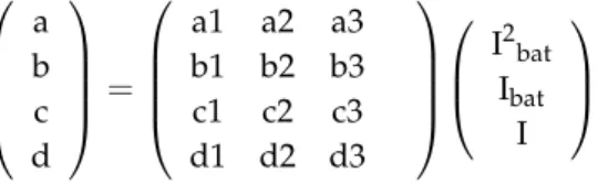
a b c d = a1 a2 a3 b1 b2 b3 c1 c2 c3 d1 d2 d3 I2bat Ibat I (14)
The calculation of a1, . . . , a3, . . . , d1, . . . , d3 in this equation is completed by the least squares fitting approach. The battery charging and discharging was tested with various currents, and the obtained results are plotted in Figure1[20].
Energies 2018, 11, x FOR PEER REVIEW 5 of 18 capacity of 4.5 Ah and a nominal voltage of 6 V. Furthermore, its charge and discharge is measured
based on a controlled current source. All the data, i.e., terminal voltage (V), current (A), as well as
SOC, are measured by the scope block. The developed data is saved in a structured format into a
MATLAB workspace, where NNs can be applied.
2.3.2. Model of Battery Floating Charge Voltage
The simulation of the battery floating charge voltage is done through the equation‐fit approach
as follows:
V′ a SOC b SOC c SOC d (12)
The voltage of the battery floating charge is represented by V′bat in this formula. This voltage
depends on the influence of temperature on the battery voltage forecast dT, which can be represented
by
V V δ T 298.15 (13)
where Vbat and δV are the calibrated voltage of the battery based on temperature influx and the
temperature factor, respectively. Moreover, the computation of the parameters introduced in
Equation (12) can be presented as follows:
I I I 3 d 2 d 1 d 3 c 2 c 1 c 3 b 2 b 1 b 3 a 2 a 1 a d c b a bat bat 2 (14)
The calculation of a1, …, a3, …, d1, …, d3 in this equation is completed by the least squares
fitting approach. The battery charging and discharging was tested with various currents, and the
obtained results are plotted in Figure 1 [20].
Figure 1. Charging of the battery and discharging validation of the floating charge voltage model. In this work, we have to solve an optimization problem minimizing the following general risk
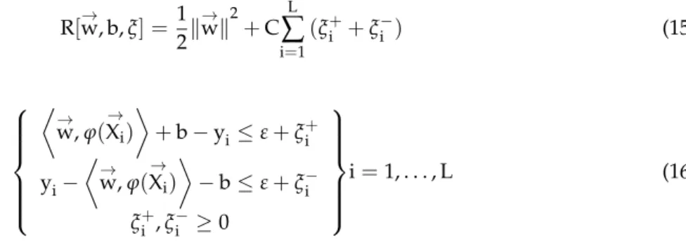
function to get the best hyper parameter value:
L 2 i i i 1 1 R [ w , b, ] w C ( ) 2
(15) subject to0 State of Charge (SOC)
2.4 B at tery Vo lt ag e ( V) 1 2 A Measured 2 A Predicted 8 A Measured 8 A Predicted 16 A Measured 16 A Predicted 20 A Measured 20 A Predicted Battery Charging Battery Dis-charging
Energies2019,12, 373 6 of 18
In this work, we have to solve an optimization problem minimizing the following general risk function to get the best hyper parameter value:
R[→w, b,ξ] = 1 2k → wk2+C L
∑
i=1 (ξi++ξ−i ) (15) subject to → w,ϕ( → Xi) +b−yi≤ε+ξi+ yi− → w,ϕ( → Xi) −b≤ε+ξi− ξ+i ,ξ−i ≥0 i=1, . . . , L (16)The first term of Equation (15) (1/2k→wk2) is applied as a measurement of function flatness. The second term is the empirical error insensitive loss function, that shows no penalty errors belowε. All the mentioned parameters are determined by the proposed optimization algorithm,
while these parameters are considered as decision variables in the optimization process to find the best optimization objective function. After the final iteration, the proposed parameters are finalized as optimal parameter values.
3. Short-Term Energy Forecasting for the Wind and PV System
The real energy control structure is depicted in Figure2. The control structure is composed of total energy generated by wind, PV, and battery resources [18–23]. Related specifications of dispatching power, the sought oscillation of output power, and also the restriction of power rate in the simulated system, have been investigated. With regards to operating conditions and the available active power, the output power from wind turbines, solar panels, and batteries is predicted in the short term. Figure2
shows the structure of the prediction equipment. In the next section, the structure of the prediction equipment will be described in detail.
Energies 2018, 11, x FOR PEER REVIEW 6 of 18
i i i i i i i i
w, (X )
b y
y
w, (X )
b
i=1,...,L
,
0
(16)The first term of Equation (15) (1/2 w 2) is applied as a measurement of function flatness. The
second term is the empirical error insensitive loss function, that shows no penalty errors below
.All the mentioned parameters are determined by the proposed optimization algorithm, while these
parameters are considered as decision variables in the optimization process to find the best
optimization objective function. After the final iteration, the proposed parameters are finalized as
optimal parameter values.
3. Short‐Term Energy Forecasting for the Wind and PV System
The real energy control structure is depicted in Figure 2. The control structure is composed of
total energy generated by wind, PV, and battery resources [18–23]. Related specifications of
dispatching power, the sought oscillation of output power, and also the restriction of power rate in
the simulated system, have been investigated. With regards to operating conditions and the available
active power, the output power from wind turbines, solar panels, and batteries is predicted in the
short term. Figure 2 shows the structure of the prediction equipment. In the next section, the structure
of the prediction equipment will be described in detail.
Figure 2. Schematic of active power control.
3.1. Construction of the Forecast Engine
One of the proper ways to simplify complex learning processes is to combine different neural
networks [18,22–24]. In the mentioned algorithm, the input data is contributed within the building
blocks; in other words, the mature distribution between these blocks. In this study, a hybrid model
of predictive tools is presented to solve this problem. This model consists of three main stages. Each
of these steps contains several layers of a multilayer perceptron (MLP) NN as a prediction tool. It
should be noted that all layers of the NN have the same features, hence the weight factor is used
directly for the next step, and it can then improve the obtained knowledge of the previous one. In the
hybrid neural network (HNN) method, using the multiple methods of MLP for the NNs increases
the learning ability. The three main layers of HNN consisting of a NN are: The LM (Levenberg– Marquardt), SCG (scaled conjugate gradient backpropagation), and CGP (conjugate gradient
backpropagation with Polak‐Ribiére updates) training approaches. Details of each layer are described
in Reference [25]. In the proposed model, the accuracy and power of prediction are increased to obtain
better results for predicting the load signal by this method. In case of choosing unsuitable values for
the weight factor of NNs, there are over‐fitting or under‐fitting problems created with the proposed
P ow er R ef ere nc e Se tti ng Dispatch Curve P t Pdispatc h Power Ramp Rate Limiter Desired Frequency Proposed Forecast Model Photovoltaic Generation Battery Generation +
Power
Allocat
ion
Wind Power Generation Ʃ + Pset delta P Pwind Ppv Pbattery P0 PCC-Figure 2.Schematic of active power control. Construction of the Forecast Engine
One of the proper ways to simplify complex learning processes is to combine different neural networks [18,22–24]. In the mentioned algorithm, the input data is contributed within the building blocks; in other words, the mature distribution between these blocks. In this study, a hybrid model of predictive tools is presented to solve this problem. This model consists of three main stages. Each of these steps contains several layers of a multilayer perceptron (MLP) NN as a prediction tool. It should be noted that all layers of the NN have the same features, hence the weight factor is used directly for the next step, and it can then improve the obtained knowledge of the previous one. In the hybrid neural network (HNN) method, using the multiple methods of MLP for the NNs increases the learning
Energies2019,12, 373 7 of 18
ability. The three main layers of HNN consisting of a NN are: The LM (Levenberg–Marquardt), SCG (scaled conjugate gradient backpropagation), and CGP (conjugate gradient backpropagation with Polak-Ribiére updates) training approaches. Details of each layer are described in Reference [25]. In the proposed model, the accuracy and power of prediction are increased to obtain better results for predicting the load signal by this method. In case of choosing unsuitable values for the weight factor of NNs, there are over-fitting or under-fitting problems created with the proposed prediction tool [26,27]. In this study, a new and upgraded HNN-based prediction tool for predicting load signals is presented to solve the problem. The proposed tool consists of combining the proposed HNN method with the new stochastic seeking approach called HBMO. Using the new hybrid method, the predictive tools training capabilities increase, and the input and output of the mapping function in a complex signal are extracted with more precision. If one of the NN members in the prediction tool falls to the lowest local area during the training, both this member and the next member is unable to escape from the trap. In order to solve this problem, the HBMO element is combined with each member of the NN of the proposed model. Therefore, in the case of the above-mentioned circumstances, the NN member has the ability to exit from these conditions.
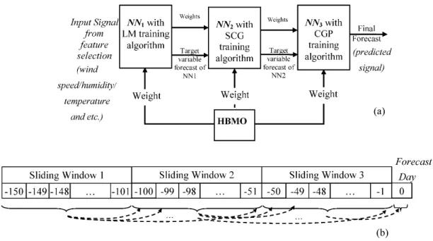
In the next step, HBMO compares the value of the target function of the current state to the previous state and selects the best value of the target function [13]. If the stop criterion is met, the next step is executed; otherwise, it returns to the previous step, the target function is calculated, and this process continues until the stop criterion is met. In the end, among the obtained values from target functions, the lowest objective function value of the HBMO algorithm is chosen as the best solution. The weight factor of the selected solution is replaced in NN1 and then the next step of the prediction tool is implemented. Once the best NN values are achieved, all members of the prediction tool are trained and selected to predict future values of the load signal. In Figure3, the prediction model is depicted. More details are given in References [28–30].
Energies 2018, 11, x FOR PEER REVIEW 7 of 18 prediction tool [26,27]. In this study, a new and upgraded HNN‐based prediction tool for predicting load signals is presented to solve the problem. The proposed tool consists of combining the proposed HNN method with the new stochastic seeking approach called HBMO. Using the new hybrid method, the predictive tools training capabilities increase, and the input and output of the mapping function in a complex signal are extracted with more precision. If one of the NN members in the prediction tool falls to the lowest local area during the training, both this member and the next member is unable to escape from the trap. In order to solve this problem, the HBMO element is combined with each member of the NN of the proposed model. Therefore, in the case of the above‐ mentioned circumstances, the NN member has the ability to exit from these conditions.
In the next step, HBMO compares the value of the target function of the current state to the previous state and selects the best value of the target function [13]. If the stop criterion is met, the next step is executed; otherwise, it returns to the previous step, the target function is calculated, and this process continues until the stop criterion is met. In the end, among the obtained values from target functions, the lowest objective function value of the HBMO algorithm is chosen as the best solution. The weight factor of the selected solution is replaced in NN1 and then the next step of the prediction tool is implemented. Once the best NN values are achieved, all members of the prediction tool are trained and selected to predict future values of the load signal. In Figure 3, the prediction model is depicted. More details are given in References [28–30].
Figure 3. The proposed forecast engine structure: (a) Main model and (b) Training mechanism. In this model, the NN output constitutes the signal forecast of the proposed model. Furthermore, in the training of this block, 50 days of historical data consisting of 50 × 24 = 1200 hourly training samples have been considered. Therefore, the main engine needs 3 × 50 = 150 days of historical data. At the beginning, the first block is trained by the historical data of 150 days ago to 101 days ago, then the second NN is trained by data from 100 days ago to 51 days ago, and finally the third block is trained by data from 50 days ago to 1 day ago. The mentioned process is frequent until the first block of the NN forecasts the signal of days −100 to −51. These signals with the selected candidates are included in sliding window 2, therefore the second NN is trained and forecasts the signal of day −50. This process will be continue to get the final output of the wind and PV signal as the predicted value.
4. Numerical Analysis
4.1. Training and Model Analysis
Figure 3.The proposed forecast engine structure: (a) Main model and (b) Training mechanism.
In this model, the NN output constitutes the signal forecast of the proposed model. Furthermore, in the training of this block, 50 days of historical data consisting of 50×24 = 1200 hourly training samples have been considered. Therefore, the main engine needs 3×50 = 150 days of historical data. At the beginning, the first block is trained by the historical data of 150 days ago to 101 days ago, then the second NN is trained by data from 100 days ago to 51 days ago, and finally the third block is trained by data from 50 days ago to 1 day ago. The mentioned process is frequent until the first block of the NN forecasts the signal of days−100 to−51. These signals with the selected candidates are
Energies2019,12, 373 8 of 18
included in sliding window 2, therefore the second NN is trained and forecasts the signal of day−50. This process will be continue to get the final output of the wind and PV signal as the predicted value.
4. Numerical Analysis
4.1. Training and Model Analysis
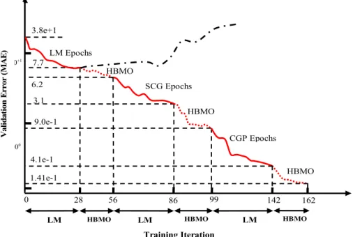
In this section, the proposed prediction tool is tested on actual information in order to investigate the effectiveness of the proposed prediction tools performance in the training phase. A usual curve based on its trial and error is shown in Figure4. In this figure, the error function is defined by mean absolute error (MAE).
Energies 2018, 11, x FOR PEER REVIEW 8 of 18 In this section, the proposed prediction tool is tested on actual information in order to investigate
the effectiveness of the proposed prediction tools performance in the training phase. A usual curve
based on its trial and error is shown in Figure 4. In this figure, the error function is defined by mean
absolute error (MAE).
In fact, this analysis is conducted to validate the planned approach around overfitting and
anachronistic convergence. It can be understood from Figure 4 that the increment of the error function
for every phase of the suggested forecast engine based on NNs leads to a stop in the learning
procedure through exchanging the last weights, which will be done based on the proposed
optimization algorithm. Therefore, the learning epochs of the learning algorithm half period for the
first three repetitions are 28, 86 – 56 = 30, and 142 – 99 = 43, which are determined by the initial
stopping model. Accordingly, production of the suggested HBMO half period in the first three
repetitions are 55 − 29 = 26, 99 – 86 = 13, and 162 − 142 = 20, which are assigned by the HBMO stopping
standards.
Additionally, to get the best effects of the proposed forecast engine structure, an additional
analysis is presented to show the optimal number of selected blocks. Accordingly, one to six blocks
of NNs have been considered here to select the best number of blocks.
Figure 4. Calculation of training results: (solid line) NN training algorithm, (dotted line) training by optimization algorithm, (dashed dotted line) overfitting of training.
In this model, we assumed that the training mechanisms of all the blocks are same. The gained
validation errors, measured in terms of mean squared error (MSE), as well as the training times, are
shown in Figure 5 a,b, respectively. In this figure, we can see that the minimum error is in NN block
number 3. Additionally, the training time is increased step by step as more NN blocks are added.
From this figure, it can be seen that an overfitting issue based on NN blocks occurs, leading to the
minimum validation error, while additional NNs cannot learn more from the input/output mapping
function of the wind and PV signal. Accordingly, three NNs are assumed for the proposed structure
with different training mechanisms to improve the performance of total training with minimum
error.
0 28 56 86 142
LM
Training Iteration
HBMO LM HBMO LM HBMO
3.8e+1 7.7 3.1 10+1 100 V alid atio n E rr or (M A E ) 99 6.2 9.0e-1 4.1e-1 162 LM Epochs SCG Epochs CGP Epochs HBMO HBMO HBMO 1.41e-1
Figure 4.Calculation of training results: (solid line) NN training algorithm, (dotted line) training by optimization algorithm, (dashed dotted line) overfitting of training.
In fact, this analysis is conducted to validate the planned approach around overfitting and anachronistic convergence. It can be understood from Figure4that the increment of the error function for every phase of the suggested forecast engine based on NNs leads to a stop in the learning procedure through exchanging the last weights, which will be done based on the proposed optimization algorithm. Therefore, the learning epochs of the learning algorithm half period for the first three repetitions are 28, 86 – 56 = 30, and 142 – 99 = 43, which are determined by the initial stopping model. Accordingly, production of the suggested HBMO half period in the first three repetitions are 55−29 = 26, 99 – 86 = 13, and 162−142 = 20, which are assigned by the HBMO stopping standards.
Additionally, to get the best effects of the proposed forecast engine structure, an additional analysis is presented to show the optimal number of selected blocks. Accordingly, one to six blocks of NNs have been considered here to select the best number of blocks.
In this model, we assumed that the training mechanisms of all the blocks are same. The gained validation errors, measured in terms of mean squared error (MSE), as well as the training times, are shown in Figure5a,b, respectively. In this figure, we can see that the minimum error is in NN block number 3. Additionally, the training time is increased step by step as more NN blocks are added. From this figure, it can be seen that an overfitting issue based on NN blocks occurs, leading to the minimum validation error, while additional NNs cannot learn more from the input/output mapping function of the wind and PV signal. Accordingly, three NNs are assumed for the proposed structure with different training mechanisms to improve the performance of total training with minimum error.
Energies2019,12, 373 9 of 18 Energies 2018, 11, x FOR PEER REVIEW 9 of 18
Figure 5. Analysis of optimal number for NN blocks: (a) Obtained validation error, and (b) training time.
Additionally, to present a proper vision of the presentation of the proposed model of the training mechanism, the first LM half cycle is continued after the early stopping point and represented by a dashed‐dotted line. The overfitting problem is solved via this procedure. As noted earlier, if a premature convergence occurs in the local minimum in this phase, LM does not have the ability to quit these conditions and causes an overfitting. Using the proposed method based on the hybrid model presented in this paper, the mentioned problem is resolved. The proposed prediction method has been applied to the obtained data from wind speed and solar radiation related to Inner Mongolia. The obtained data is used as real data to model wind speed and solar radiation. This data is plotted in Figure 6.
To validate the authenticity of the suggested method, diverse error standards, such as MAE, root mean square error (RMSE), and normalized mean absolute percentage error (NMAPE), are considered in this case study. The pertaining formulas of these error standards are as follows:
f r N i i r i 1 i PV PV 100 NMAPE 100% N PV
(17)The amount of data is represented by N in this formula. The predicted data of PV energy and the actual data of PV energy are determined by f
i
PV and a i
PV , respectively. Bar notation represents the mean of these values.
N f r i i i 1 1 MAE PV PV N
(18)
2 N f r i i i 1 1 RMSE PV PV N
(19)Figure 5. Analysis of optimal number for NN blocks: (a) Obtained validation error, and (b) training time.
Additionally, to present a proper vision of the presentation of the proposed model of the training mechanism, the first LM half cycle is continued after the early stopping point and represented by a dashed-dotted line. The overfitting problem is solved via this procedure. As noted earlier, if a premature convergence occurs in the local minimum in this phase, LM does not have the ability to quit these conditions and causes an overfitting. Using the proposed method based on the hybrid model presented in this paper, the mentioned problem is resolved. The proposed prediction method has been applied to the obtained data from wind speed and solar radiation related to Inner Mongolia. The obtained data is used as real data to model wind speed and solar radiation. This data is plotted in Figure6.
To validate the authenticity of the suggested method, diverse error standards, such as MAE, root mean square error (RMSE), and normalized mean absolute percentage error (NMAPE), are considered in this case study. The pertaining formulas of these error standards are as follows:
NMAPE= 100 N N
∑
i=1 PV f i−PVri PV r i ×100% (17)The amount of data is represented by N in this formula. The predicted data of PV energy and the actual data of PV energy are determined by PVfi and PVai, respectively. Bar notation represents the mean of these values.
MAE= 1 N N
∑
i=1 PV f i−PVri (18) RMSE= v u u t1 N N∑
i=1 PVfi−PVri 2 (19)Energies2019,12, 373 10 of 18 Energies 2018, 11, x FOR PEER REVIEW 10 of 18
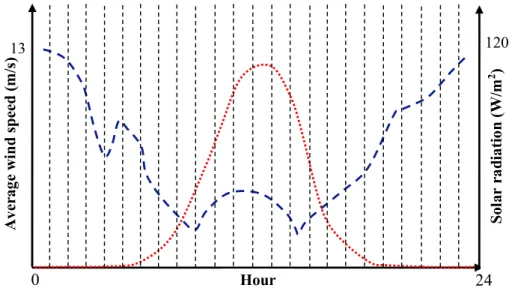
Figure 6. Wind speed trend and solar radiation curve. Red dotted line, PV; blue dashed line, wind.
4.2. Obtained Results for the Forecast Engine
In order to compare the performance of the proposed method with other methods under
equivalent circumstances, the modeling results were compared with the results presented in
Reference [6]. The obtained results from the proposed method in comparison with the other four
methods presented in Reference [6] are listed in Table 1.
Table 1. Generated numerical results of the suggested forecasting model in comparison with other strategies.
Methods Error
Winter Spring Summer Fall
23 December 5 December 12 May 27 April 26 June 27 August 18 October 28 September BPNN [6] NMAPE 29.65 35.47 18.55 23.45 21.05 18.67 15.17 32.74 MAE 1.08 1.47 1.56 1.98 1.88 1.35 0.81 2.01 RMSE 1.92 2.15 2.04 2.73 2.20 1.86 0.96 2.68 RBFNN [6] NMAPE 16.71 35.46 17.24 18.21 10.84 5.12 7.22 21.86 MAE 0.61 1.47 1.45 1.54 0.94 0.37 0.38 1.34 RMSE 0.74 1.72 1.94 2.20 1.43 0.45 0.49 1.80 WT + BPNN [6] NMAPE 11.94 30.26 16.99 17.95 17.62 5.98 13.07 22.44 MAE 0.43 1.25 1.44 1.51 1.54 0.43 0.70 1.38 RMSE 0.62 1.66 1.70 1.89 2.05 0.55 0.79 1.52 WT + RBFNN [6] NMAPE 8.16 13.81 8.91 13.14 8.54 4.25 4.32 12.17 MAE 0.29 0.57 0.75 1.11 0.74 0.30 0.23 0.75 RMSE 0.40 0.64 1.01 1.57 1.06 0.38 0.32 0.87 Proposed NMAPE 7.13 10.56 6.78 10.47 6.2 3.46 3.4 9.84 MAE 0.26 0.51 0.62 1 0.73 0.3 0.28 0.61 RMSE 0.36 0.45 0.9 1.31 0.84 0.25 0.33 0.7 By examining the obtained results from Table 1, it can be stated that the performance of the
proposed method is better than the other four methods in terms of all the error criteria. In order to
demonstrate the superiority of the active power distribution method in comparison with the classical
mean method, the effect of the proposed active power method for controlling the active power of the
network and supplying the network power in two modes was investigated. The two cases are: (a)
The energy storing batteries were not complicated in active power control, and (b) the energy storing
batteries were complex in active power control.
4.3. Test Cases in the Power System
Case one: In this case, the forecasted output power of the proposed strategy through the high‐
level network is a stationary signal, as shown in Figure 7. The minimum and maximum power is
0
Hour 13 A ver ag e w ind speed ( m /s )24
120 S ol ar ra di at io n (W /m 2 )Figure 6.Wind speed trend and solar radiation curve. Red dotted line, PV; blue dashed line, wind. 4.2. Obtained Results for the Forecast Engine
In order to compare the performance of the proposed method with other methods under equivalent circumstances, the modeling results were compared with the results presented in Reference [6]. The obtained results from the proposed method in comparison with the other four methods presented in Reference [6] are listed in Table1.
Table 1. Generated numerical results of the suggested forecasting model in comparison with other strategies.
Methods Error
Winter Spring Summer Fall
23 December 5 December 12 May 27 April 26 June 27 August 18 October 28 September BPNN [6] NMAPE 29.65 35.47 18.55 23.45 21.05 18.67 15.17 32.74 MAE 1.08 1.47 1.56 1.98 1.88 1.35 0.81 2.01 RMSE 1.92 2.15 2.04 2.73 2.20 1.86 0.96 2.68 RBFNN [6] NMAPE 16.71 35.46 17.24 18.21 10.84 5.12 7.22 21.86 MAE 0.61 1.47 1.45 1.54 0.94 0.37 0.38 1.34 RMSE 0.74 1.72 1.94 2.20 1.43 0.45 0.49 1.80 WT + BPNN [6] NMAPE 11.94 30.26 16.99 17.95 17.62 5.98 13.07 22.44 MAE 0.43 1.25 1.44 1.51 1.54 0.43 0.70 1.38 RMSE 0.62 1.66 1.70 1.89 2.05 0.55 0.79 1.52 WT + RBFNN [6] NMAPE 8.16 13.81 8.91 13.14 8.54 4.25 4.32 12.17 MAE 0.29 0.57 0.75 1.11 0.74 0.30 0.23 0.75 RMSE 0.40 0.64 1.01 1.57 1.06 0.38 0.32 0.87 Proposed NMAPE 7.13 10.56 6.78 10.47 6.2 3.46 3.4 9.84 MAE 0.26 0.51 0.62 1 0.73 0.3 0.28 0.61 RMSE 0.36 0.45 0.9 1.31 0.84 0.25 0.33 0.7
By examining the obtained results from Table1, it can be stated that the performance of the proposed method is better than the other four methods in terms of all the error criteria. In order to demonstrate the superiority of the active power distribution method in comparison with the classical mean method, the effect of the proposed active power method for controlling the active power of the network and supplying the network power in two modes was investigated. The two cases are: (a) The energy storing batteries were not complicated in active power control, and (b) the energy storing batteries were complex in active power control.
4.3. Test Cases in the Power System
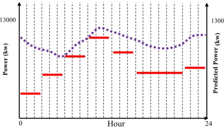
Case one: In this case, the forecasted output power of the proposed strategy through the high-level network is a stationary signal, as shown in Figure7. The minimum and maximum power is equal to
Energies2019,12, 373 11 of 18
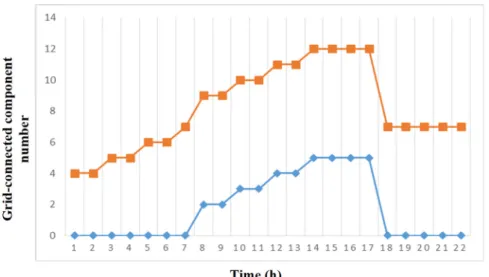
2000 and 1000 kW, respectively, and shifts occur at 3, 5, 10, 13, 15, and 20 h. In this test case, the outputs of the wind-solar battery power system generated through the average model and the suggested power placement method were compared by the anticipated output power. Regarding this mode, the error of the output power was lower and the output power curve was flatter than that of the average method. In this test case, the max tracking error as well as the mean square of the tracking error provided by the suggested method are 889.7 and 339.6 kW, respectively. Moreover, the suggested model outperformed the conventional model. Additionally, regarding this system (considering wind and PV), the PV modules were not permitted to launch until the modifiable ability of the wind turbines was insufficient to meet the desired output power. In Figure8, the simulation results of the network connected to the wind turbine and the photovoltaic panels are shown. It is assumed that the maximum capacity of the wind turbine for power extraction is used; that is, when the wind turbine does not have the required power to provide the maximum capacity, the solar system is operational. It can be stated that when the number of solar modules in a connected network is greater than zero, the number of wind turbines is equal to 8. By analyzing Figure9, the number of on/off switches in the proposed method is lower than the mean model in all stages of the modulation test.
In the second test case, the predicted output power of the proposed strategy through the high-level network is a stationary signal, as shown in Figure7. The minimum power and maximum power is equal to 4000 and 11,000 kW, respectively, and shifts occur at 3, 5, 11, 16, and 19 h. During daily performance of the complex method, the demand path of the output power has been determined. In Figure9, the output power of the proposed complex method assessed via the power allocation method is related to the predicted output power.
Energies 2018, 11, x FOR PEER REVIEW 11 of 18 equal to 2000 and 1000 kW, respectively, and shifts occur at 3, 5, 10, 13, 15, and 20 h. In this test case,
the outputs of the wind‐solar battery power system generated through the average model and the
suggested power placement method were compared by the anticipated output power. Regarding this
mode, the error of the output power was lower and the output power curve was flatter than that of
the average method. In this test case, the max tracking error as well as the mean square of the tracking
error provided by the suggested method are 889.7 and 339.6 kW, respectively. Moreover, the
suggested model outperformed the conventional model. Additionally, regarding this system
(considering wind and PV), the PV modules were not permitted to launch until the modifiable ability
of the wind turbines was insufficient to meet the desired output power. In Figure 8, the simulation
results of the network connected to the wind turbine and the photovoltaic panels are shown. It is
assumed that the maximum capacity of the wind turbine for power extraction is used; that is, when
the wind turbine does not have the required power to provide the maximum capacity, the solar
system is operational. It can be stated that when the number of solar modules in a connected network
is greater than zero, the number of wind turbines is equal to 8. By analyzing Figure 9, the number of
on/off switches in the proposed method is lower than the mean model in all stages of the modulation
test.
In the second test case, the predicted output power of the proposed strategy through the high‐
level network is a stationary signal, as shown in Figure 7. The minimum power and maximum power
is equal to 4000 and 11,000 kW, respectively, and shifts occur at 3, 5, 11, 16, and 19 h. During daily
performance of the complex method, the demand path of the output power has been determined. In
Figure 9, the output power of the proposed complex method assessed via the power allocation
method is related to the predicted output power.
Figure 7. Wind speed trend and solar radiation curve. Red dotted line, PV; blue dashed line, wind. As illustrated in Figure 9, if the sum of the forecast energy obtained from wind turbines and
photovoltaic panels is more than the predicted output energy, then the output of the whole system is
controlled using the suggested appropriation method and can track the sought energy. It is
remarkable that the output energy curve is flat and without oscillation. Earlier, when the whole
predicted power was lower than the predicted output power, the batteries were allowed to unload.
As shown in Figure 9, this procedure was continued until the battery’s SOC reached SOCmin.
Therefore, the desired power can be tracked using the suggested approach, until the battery SOC is
higher than SOCmin. Subsequently, to improve the usage of the wind and solar power generators for
the equipment, when SOC is lower than SOCmin, the wind power and photovoltaic panels have the
highest power output of the predicted power. 0 13000 P ower ( kw ) 24 1300 P redi cte d P ower ( k w 2)
Hour
(kw)Figure 7.Wind speed trend and solar radiation curve. Red dotted line, PV; blue dashed line, wind.
As illustrated in Figure9, if the sum of the forecast energy obtained from wind turbines and photovoltaic panels is more than the predicted output energy, then the output of the whole system is controlled using the suggested appropriation method and can track the sought energy. It is remarkable that the output energy curve is flat and without oscillation. Earlier, when the whole predicted power was lower than the predicted output power, the batteries were allowed to unload. As shown in Figure9, this procedure was continued until the battery’s SOC reached SOCmin. Therefore, the desired power can be tracked using the suggested approach, until the battery SOC is higher than SOCmin. Subsequently, to improve the usage of the wind and solar power generators for the equipment, when SOC is lower than SOCmin, the wind power and photovoltaic panels have the highest power output of the predicted power.
Energies2019,12, 373 12 of 18 Energies 2018, 11, x FOR PEER REVIEW 12 of 18
Figure 8. The statistics of component numbers connected to the grid based on the suggested model.
Figure 9. SOC of the energy storage battery.
4.3. Optimization Analysis
In this section, an additional analysis is provided to show the effectiveness of the proposed
optimization algorithm. In order to find out why HBMO is used to solve this problem instead of
many other optimization algorithms, an optimization analysis is presented to prove the advantages
and ability of HBMO [31].
The Ackley benchmark function, which is the reference of the data, is considered to show the
effectiveness of the proposed optimization method [32]. This function is formulated as follows:
2 2 2 xi cos( c . x )i i 1 i 1 b . 1 n n 1 2 i f (x , x ) a.e e a e a =20, b =0.2, c=2 , 20 x 20, i 1, 2
(20)In this function, the target is getting the minimum value, and as can be seen in Table 2, the best
results are yielded by HBMO compared to the other optimization algorithms, namely the
evolutionary algorithm [33], genetic algorithm (GA) [34], differential evolutionary (DE) algorithm
[35], ant colony (ACO) algorithm [36], and particle swarm optimization (PSO) [37]. In Table 2,
minimum, maximum, and mean values for all optimization algorithms are presented through an
equal number of trial runs—10 trials. As shown in this table, the proposed optimization algorithm
could provide better results.
Figure 8.The statistics of component numbers connected to the grid based on the suggested model.
Energies 2018, 11, x FOR PEER REVIEW 12 of 18
Figure 8. The statistics of component numbers connected to the grid based on the suggested model.
Figure 9. SOC of the energy storage battery.
4.3. Optimization Analysis
In this section, an additional analysis is provided to show the effectiveness of the proposed
optimization algorithm. In order to find out why HBMO is used to solve this problem instead of
many other optimization algorithms, an optimization analysis is presented to prove the advantages
and ability of HBMO [31].
The Ackley benchmark function, which is the reference of the data, is considered to show the
effectiveness of the proposed optimization method [32]. This function is formulated as follows:
2 2 2 xi cos( c . x )i i 1 i 1 b . 1 n n 1 2 i f (x , x ) a.e e a e a =20, b =0.2, c=2 , 20 x 20, i 1, 2
(20)In this function, the target is getting the minimum value, and as can be seen in Table 2, the best
results are yielded by HBMO compared to the other optimization algorithms, namely the
evolutionary algorithm [33], genetic algorithm (GA) [34], differential evolutionary (DE) algorithm
[35], ant colony (ACO) algorithm [36], and particle swarm optimization (PSO) [37]. In Table 2,
minimum, maximum, and mean values for all optimization algorithms are presented through an
equal number of trial runs—10 trials. As shown in this table, the proposed optimization algorithm
could provide better results.
Figure 9.SOC of the energy storage battery. 4.4. Optimization Analysis
In this section, an additional analysis is provided to show the effectiveness of the proposed optimization algorithm. In order to find out why HBMO is used to solve this problem instead of many other optimization algorithms, an optimization analysis is presented to prove the advantages and ability of HBMO [31].
The Ackley benchmark function, which is the reference of the data, is considered to show the effectiveness of the proposed optimization method [32]. This function is formulated as follows:
f(x1, x2) =−a.e −b. v u u t 2 ∑ i=1x2i n −e 2 ∑ i=1 cos(c.xi) n +a+e1 a=20, b=0.2, c=2×π,−20≤xi≤20, i=1, 2 (20)
In this function, the target is getting the minimum value, and as can be seen in Table 2, the best results are yielded by HBMO compared to the other optimization algorithms, namely the evolutionary algorithm [33], genetic algorithm (GA) [34], differential evolutionary (DE) algorithm [35], ant colony (ACO) algorithm [36], and particle swarm optimization (PSO) [37]. In Table2, minimum, maximum, and mean values for all optimization algorithms are presented through an equal number
Energies2019,12, 373 13 of 18
of trial runs—10 trials. As shown in this table, the proposed optimization algorithm could provide better results.
Table 2.Obtained results for the Ackley benchmark function.
Index EA GA DE ACO PSO Proposed
MIN 3.14×10⁻⁸ 6.15×10⁻⁹ 5.21×10⁻¹⁴ 4.87×10⁻¹⁴ 0.00 0.00 MEAN 2.031 0.583 5.02×10⁻¹ 5.09×10⁻¹ 3.05×10⁻¹ 1.53×10−2
MAX 4.182 4.361 1.572 8.54×10⁻¹ 7.30×10⁻¹ 5.81×10⁻²
To show the graphical representation of the proposed benchmark function, the Ackley function is presented in Figure10. This figure is plotted in the feasible region of −20 to 20 for x1 and x2. In Figure11, the proposed optimization algorithm is compared with the five other algorithms in terms of iteration speed and final optimal values. As presented in this figure, the proposed method and the other five obtained results in the first iteration (section A) and the last iteration (section B) are presented. All figures demonstrate the validity and superiority of the proposed algorithm in comparison with others. In this problem, the number of iterations and the population were set to 50 and 10, respectively.
Energies 2018, 11, x FOR PEER REVIEW 13 of 18
Table 2. Obtained results for the Ackley benchmark function.
Index EA GA DE ACO PSO Proposed
MIN 3.14 × 10⁻⁸ 6.15 × 10⁻⁹ 5.21 × 10⁻¹⁴ 4.87 × 10⁻¹⁴ 0.00 0.00
MEAN 2.031 0.583 5.02 × 10⁻¹ 5.09 × 10⁻¹ 3.05 × 10⁻¹ 1.53 × 10−2
MAX 4.182 4.361 1.572 8.54 × 10⁻¹ 7.30 × 10⁻¹ 5.81 × 10⁻²
To show the graphical representation of the proposed benchmark function, the Ackley function is presented in Figure 10. This figure is plotted in the feasible region of −20 to 20 for x1 and x2. In
Figure 11, the proposed optimization algorithm is compared with the five other algorithms in terms of iteration speed and final optimal values. As presented in this figure, the proposed method and the other five obtained results in the first iteration (section A) and the last iteration (section B) are presented. All figures demonstrate the validity and superiority of the proposed algorithm in comparison with others. In this problem, the number of iterations and the population were set to 50 and 10, respectively.
Figure 10. The proposed Ackley function.
Figure 11. Optimization algorithm on Ackley function: Values of the first iterations for the algorithms: A1 (Proposed), A2 (PSO), A3 (DE), A4 (ACO), A5 (GA), and A6 (EA). Values of the final iteration: B1
(Proposed), B2 (PSO), B3 (DE), B4 (ACO), B5 (GA), and B6 (EA).
-20 0 20 X1 -20 0 20 X 2 -20 0 20 X1 -20 0 20 X2 -20 0 20 X1 -20 0 20 X2 -20 0 20 X1 -20 0 20 X 2 -20 0 20 X1 -20 0 20 X 2 -20 0 20 X1 -20 0 20 X2 -20 0 20 X1 -20 0 20 X 2 -20 0 20 X1 -20 0 20 X2 -20 0 20 X1 -20 0 20 X 2 -20 0 20 X1 -20 0 20 X 2 -20 0 20 X1 -20 0 20 X2 -20 0 20 X1 -20 0 20 X2 A1 A2 A3 A4 A5 A6 B1 B2 B3 B4 B5 B6
Figure 10.The proposed Ackley function.
Energies 2018, 11, x FOR PEER REVIEW 13 of 18
Table 2. Obtained results for the Ackley benchmark function.
Index EA GA DE ACO PSO Proposed
MIN 3.14 × 10⁻⁸ 6.15 × 10⁻⁹ 5.21 × 10⁻¹⁴ 4.87 × 10⁻¹⁴ 0.00 0.00
MEAN 2.031 0.583 5.02 × 10⁻¹ 5.09 × 10⁻¹ 3.05 × 10⁻¹ 1.53 × 10−2
MAX 4.182 4.361 1.572 8.54 × 10⁻¹ 7.30 × 10⁻¹ 5.81 × 10⁻²
To show the graphical representation of the proposed benchmark function, the Ackley function is presented in Figure 10. This figure is plotted in the feasible region of −20 to 20 for x1 and x2. In
Figure 11, the proposed optimization algorithm is compared with the five other algorithms in terms of iteration speed and final optimal values. As presented in this figure, the proposed method and the other five obtained results in the first iteration (section A) and the last iteration (section B) are presented. All figures demonstrate the validity and superiority of the proposed algorithm in comparison with others. In this problem, the number of iterations and the population were set to 50 and 10, respectively.
Figure 10. The proposed Ackley function.
Figure 11. Optimization algorithm on Ackley function: Values of the first iterations for the algorithms: A1 (Proposed), A2 (PSO), A3 (DE), A4 (ACO), A5 (GA), and A6 (EA). Values of the final iteration: B1
(Proposed), B2 (PSO), B3 (DE), B4 (ACO), B5 (GA), and B6 (EA).
-20 0 20 X1 -20 0 20 X 2 -20 0 20 X1 -20 0 20 X2 -20 0 20 X1 -20 0 20 X2 -20 0 20 X1 -20 0 20 X 2 -20 0 20 X1 -20 0 20 X 2 -20 0 20 X1 -20 0 20 X 2 -20 0 20 X1 -20 0 20 X 2 -20 0 20 X1 -20 0 20 X2 -20 0 20 X1 -20 0 20 X 2 -20 0 20 X1 -20 0 20 X 2 -20 0 20 X1 -20 0 20 X2 -20 0 20 X1 -20 0 20 X 2 A1 A2 A3 A4 A5 A6 B1 B2 B3 B4 B5 B6
Figure 11.Optimization algorithm on Ackley function: Values of the first iterations for the algorithms: A1(Proposed), A2(PSO), A3(DE), A4(ACO), A5(GA), and A6(EA). Values of the final iteration: B1
Energies2019,12, 373 14 of 18
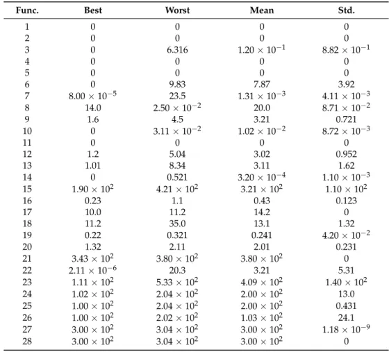
Furthermore, to show the abilities of the proposed method, different mathematical benchmarks of CEC2013 have been considered, including 28 problems. In this analysis, 10, 30, and 50 dimensions, as well as the complexity of the algorithm, were evaluated. The proposed benchmarks include F1 to F5 as unimodal functions, F6 to F20 as multimodal functions, and F21 to F28 as composite functions. The obtained results of the proposed algorithm over the mentioned benchmarks in 10-D, 30-D, and 50-D are presented in Tables3–5, respectively.
Table 3.Obtained numerical results for D = 10.
Func. Best Worst Mean Std.
1 0 0 0 0 2 0 0 0 0 3 0 6.316 1.20×10⁻¹ 8.82×10⁻¹ 4 0 0 0 0 5 0 0 0 0 6 0 9.83 7.87 3.92 7 8.00×10⁻⁵ 23.5 1.31×10⁻³ 4.11×10⁻³ 8 14.0 2.50×10⁻² 20.0 8.71×10⁻² 9 1.6 4.5 3.21 0.721 10 0 3.11×10⁻² 1.02×10⁻² 8.72×10⁻³ 11 0 0 0 0 12 1.2 5.04 3.02 0.952 13 1.01 8.34 3.11 1.62 14 0 0.521 3.20×10⁻⁴ 1.10×10⁻³ 15 1.90×10² 4.21×10² 3.21×10² 1.10×10² 16 0.23 1.1 0.43 0.123 17 10.0 11.2 14.2 0 18 11.2 35.0 13.1 1.32 19 0.22 0.321 0.241 4.20×10⁻² 20 1.32 2.11 2.01 0.231 21 3.43×10² 3.80×10² 3.80×10² 0 22 2.11×10⁻⁶ 20.3 3.21 5.31 23 1.11×10² 5.33×10² 4.09×10² 1.40×10² 24 1.02×10² 2.04×10² 2.00×10² 13.0 25 1.00×10² 2.04×10² 2.00×10² 0.431 26 1.00×10² 2.02×10² 1.03×10² 24.1 27 3.00×10² 3.04×10² 3.00×10² 1.18×10⁻⁹ 28 3.00×10² 3.04×10² 3.00×10² 0
Table 4.Obtained numerical results for D = 30.
Func. Best Worst Mean Std.
1 0 0 0 0 2 1.22×10³ 4.10×10⁴ 8.00×10³ 6.41×10³ 3 0 1.20×10³ 34.1 1.51×10² 4 5.33×10⁻⁷ 0.12 1.51×10⁻⁴ 2.42×10⁻⁴ 5 0 0 0 0 6 0 22.1 0.434 2.41 7 0.412 22.1 3.44 4.21 8 20.1 21.0 20.6 1.31×10⁻⁵
Energies2019,12, 373 15 of 18
Table 4.Cont.
Func. Best Worst Mean Std.
9 21.2 30.3 23.3 1.21 10 1.30×10⁻² 0.165 5.45×10⁻² 2.31×10⁻² 11 0 0 0 0 12 11.6 31.2 21.3 3.13 13 21.6 73.0 43.4 11.1 14 0 0.101 2.32×10⁻² 1.41×10⁻² 15 2.14×10³ 3.20×10³ 2.51×10³ 2.10×10² 16 6.54×10⁻² 1.11 0.841 0.1 17 10.2 23.2 25.2 2.40×10⁻¹⁵ 18 23.2 83.4 66.1 2.32 19 0.652 1.32 1.20 1.30×10⁻² 20 5.41 11.3 10.1 2.30×10⁻² 21 2.00×10² 4.12×10² 2.52×10² 32.1 22 10.1 1.03×10² 7.52×10² 13.1 23 2.11×10³ 3.34×10³ 3.21×10² 23.1 24 2.00×10² 2.23×10² 2.00×10² 4.31 25 2.00×10² 2.43×10² 2.31×10² 14.1 26 2.00×10² 3.01×10² 2.01×10² 12.0 27 3.00×10² 6.34×10² 3.40×10² 14.1 28 3.00×10² 3.00×10² 3.00×10² 0
Table 5.Obtained numerical results for D = 50.
Func. Best Worst Mean Std.
1 0 0 0 0 2 4.32×10³ 4.53×10⁴ 2.30×10³ 1.12×10⁴ 3 1.43 6.54×10⁵ 5.40×10⁵ 1.42×10⁵ 4 2.52×10⁻⁶ 5.32×10⁻³ 1.33×10⁻² 1.31×10⁻³ 5 0 0 0 0 6 2.32 32.4 33.8 1.31×10⁻² 7 6.50 45.5 4.32 8 10.0 14.2 2.09 1.30×10⁻² 9 30.0 45.5 23.9 1.12 10 6.50×10⁻³ 0.00 4.48×10⁻² 2.23×10⁻² 11 0 0.00 0 0 12 25.0 50.0 42.9 10.1 13 11.0 1.37×10² 1.11×10⁻² 12.6 14 0 5.45×10⁻² 2.46×10⁻² 11.7 15 3.30×10³ 4.24×10³ 5.34×10³ 2.38×10² 16 0.23 1.23 1.26 0.139 17 32.4 42.5 43.4 3.16×10⁻¹⁵ 18 12.3 1.26×10² 1.23×10² 1.64 19 1.40 2.33 2.37 0.141 20 13.0 20.7 15.5 0.528 21 2.00×10² 1.18×10³ 4.33×10² 2.41×10² 22 7.40 43.5 12.7 5.31 23 4.50×10³ 5.38×10³ 4.52×10³ 4.21×10² 24 21.0 2.35×10² 1.48×10³ 1.02 25 2.20×10² 3.47×10² 3.23×10² 2.41 26 2.00×10² 3.26×10² 2.17×10² 4.40 27 5.12×10² 1.35×10³ 5.33×10² 34.0 28 4.04×10² 2.67×10³ 3.54×10² 34.0
Energies2019,12, 373 16 of 18
5. Conclusions
In this work, a novel method for controlling the output power of renewable energy sources using an intelligent algorithm is presented. The parameters which are predicted in this model are the output power of wind and solar power generators. This paper presents a new model based on a combination of solar and wind, as well as a battery storage system. Additionally, the proposed solution method is framed to adjust the output power of the proposed system to obtain the reference power ordered by the grid, in which the amount of on/off and off/on switching of renewable energy sources is minimized and the application of the regulation ability of wind turbines is maximized. Specifically, the forecasted power of these signals is taken as the production aptitude of wind turbines and PV. Furthermore, a new forecasting tool based on the artificial prediction tool has been introduced to predict wind and solar signals. The prediction model is inspired by the performance of the HBMO algorithm. In this model, free parameters in the multi-stage forecasting tool in the learning mechanism are optimized. One of the optimization issues is the ability to locate active power. The proposed algorithm is looking for the best answer. The validity and advantages of the proposed method have been examined by considering factors such as output power performance, the reduction degree of change, and maintaining SOC at the same time. The superiority of the proposed method has been proven in comparison with other methods. Through this method, the maximum output power of the wind turbine, and a reduction in the number of on/off switches with respect to PV, are obtained.
Author Contributions:Conceptualization, M.B. and M.S.N. (Mohammad Salay Naderi); Methodology, O.A. and N.G.; Software, O.A. and V.N.; Validation, M.S.N. (Mehdi Salay Naderi); Writing-Original Draft Preparation, O.A., M.B., N.G. and V.N.; Writing–Review & Editing, M.S.N. (Mohammad Salay Naderi) and M.S.N. (Mehdi Salay Naderi).
Funding: This research was funded by Faculty Development Competitive Research Grant of Nazarbayev University grant number SOE2018018.
Conflicts of Interest:The authors declare no conflict of interest.
References
1. Manla, E.; Nasiri, A.; Rentel, C.H.; Hughes, M. Modeling of Zinc/Bromide Energy Storage for Vehicular Applications.IEEE Trans. Ind. Electron.2010,57, 624–632. [CrossRef]
2. Wang, J.; Shahidehpour, M.; Li, Z. Security-constrained unit commitment with volatile wind power generation.IEEE Trans. Power Syst.2008,23, 1319–1327. [CrossRef]
3. Ummels, B.C.; Gibescu, M.; Pelgrum, E.; Kling, W.L.; Brand, A.J. Impacts of wind power on thermal generation unit commitment and dispatch.IEEE Trans. Energy Convers.2007,22, 44–51. [CrossRef]
4. Jiang, R.; Wang, J.; Guan, Y. Robust unit commitment with wind power and pumped storage hydro. IEEE Trans. Power Syst.2012,27, 800. [CrossRef]
5. Teleke, S.; Baran, M.; Bhattacharya, S.; Huang, A. Optimal control of battery energy storage for wind farm dispatching.IEEE Trans. Energy Convers.2010,25, 787–794. [CrossRef]
6. Mandal, P.; Madhira, S.T.S.; Haque, A.U.; Meng, J.; Pineda, R.L. Forecasting Power Output of Solar Photovoltaic System Using Wavelet Transform and Artificial Intelligence Techniques. Procedia Comput. Sci.2012,12, 332–337. [CrossRef]
7. Abedinia, O.; Amjady, N.; Ghadimi, N. Solar energy forecasting based on hybrid neural network and improved metaheuristic algorithm.Comput. Intell.2017,34, 241–260. [CrossRef]
8. Abedinia, O.; Raisz, O.; Amjady, N. An Effective Prediction Model for Hungarian Small-Scale Solar Power Output.IET Renew. Power Gener.2017,11, 1648–1658. [CrossRef]
9. Bhangu, B.; Bentley, P.; Stone, D.; Bingham, C. Nonlinear observers for predicting state-of-charge and state-of-health of lead-acid batteries for hybrid-electric vehicles.IEEE Trans. Veh. Technol.2005,54, 783–794. [CrossRef]
10. Rodrigues, E.M.G.; Godina, R.; Catalão, J.P.S. Modelling electrochemical energy storage devices in insular power network applications supported on real data.Appl. Energy2017,188, 315–329. [CrossRef]