Gyper: A graph-based HLA genotyper using aligned DNA sequences

(1)

Faculty of Industrial Engineering, Mechanical Engineering and Computer

Science

Faculty of Industrial Engineering, Mechanical Engineering and Computer

Science

Gyper: A graph-based HLA genotyper

using aligned DNA sequences

(2)

(3)

GYPER: A GRAPH-BASED HLA GENOTYPER USING

ALIGNED DNA SEQUENCES

Hannes Pétur Eggertsson

60 ECTS thesis submitted in partial fulfillment of a Magister Scientiarum degree in computational engineering

Advisors

Bjarni Vilhjálmur Halldórsson (deCODE genetics)

Páll Melsted (University of Iceland)

Faculty Representative

Daníel Fannar Guðbjartsson

Faculty of Industrial Engineering, Mechanical Engineering and Computer

Science

School of Engineering and Natural Sciences

University of Iceland

(4)

Gyper: A graph-based HLA genotyper using aligned DNA sequences Gyper

Faculty of Industrial Engineering, Mechanical Engineering and Computer Science School of Engineering and Natural Sciences

University of Iceland Hjarðarhaga 2-6 107, Reykjavík, Reykjavik Iceland Telephone: 525 4700 Bibliographic information:

Hannes Pétur Eggertsson, 2015, Gyper: A graph-based HLA genotyper using aligned DNA sequences, M.Sc. thesis, Faculty of Industrial Engineering, Mechanical Engineering and Com-puter Science, University of Iceland.

Printing: Háskólaprent, Fálkagata 2, 107 Reykjavík Reykjavik, Iceland, September 2015

(5)

List of Figures

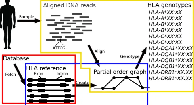
1.1 The flow of information within an eukaryotic cell system. The coding sequence for the proteins are the red, green, and blue regions. Exons are spliced together to form RNA which is translated to protein. . . 2 1.2 Overview of Gyper’s genotyping pipeline. An individual is sampled and

se-quenced. The sequenced reads are aligned to the human reference genome. The HLA allele references are fetched from an external database. A partial order graph is created which stores all the alleles in a single graph for each gene. Finally, we align the sequenced reads to the graph and genotype the individual. . . 6

2.1 A read pair. The two reads are read from one end of each fragment strands in opposite direction. . . 7 2.2 Two chromosome strands. A is always bonded with T and C is bonded

with G. The reverse complementary of the sequence GATACCC is GGGTATC. . 8 2.3 Example FASTA file entry for a sequence from the human reference genome.

Here the sequence ID is chr6_7500001-7500350 meaning the sequence is from chromosome 6 and is showing bases located at 7500001 to 7500350. The sequence description is omitted. Following the header is the sequencing data split by 50 characters per line. . . 10 2.4 An example of a reference allele format. . . 12

3.1 Modified version of Gyper’s pipeline (Figure 1.2). The scope of the three main steps are highlighted. . . 15 3.2 IMGT/HLA XML wrapper example output. . . 16 3.3 Flow chart for finding relevant positions of the human genome using one

al-lele. Reads overlapping the exons are simulated and mapped to the human reference genome. . . 18

(8)

LIST OF FIGURES

3.4 Example input and output of our MSA. Bases colored green and red are

indels (insertions or deletions) and mismatches, respectively. . . 22

3.5 Create a partial order reference graph using three example exon sequences: GATA,-AT-, and CATA. Blue edges show edges we traversed through, green labels represent changed or new labels on edges. Red and yellow nodes represent new and old nodes, respectively. a) Two nodes are created, initial node on level 0 and a final node on levelLength(sequences[0]) + 1, which is here 5. b) The sequence GATA is added to the graph. c) The sequence -AT- is added to the graph. Note that no new nodes need to be created, only edges. We change the bit string for the edge going from A to T so it includes this sequence. d) The sequence CATA is added to the graph. The new C node will be on the same level as the G node. . . 25

3.6 Extended graph from figure 3.5. Here we have added three intron references to the graph. We use the previous initial node as a final node for the new extension. The red nodes are the new intron nodes. The intron sequences we have added are: TTA, GTA, and -TA. Note that the edges on the new nodes do not store a bit string like the other exon nodes. . . 27

3.7 Alignment of the sequenceACATto the graph from figure 3.6. The numbers below each node denotes their topological sort order and blue edges are the path of the alignment. . . 31

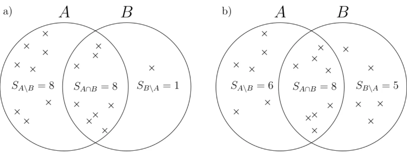
3.8 Alleles A and B are represented as sets. Each set has the reads that allele explains. The number of reads explained by either allele A or B is SA,B =SA\B+SA∩B+SB\A. . . 35

3.9 Two examples of the distributions of reads (crosses) among two alleles, A and B. a) It is likely that the individual is homozygous even though SA= 16 and SA,B = 17. The read inside the B\A region is likely an error. b) Here however, SA\B and SB\A are relatively similar and thus we would rather expect that the individual is heterozygous. . . 36

4.1 Coverage plot forHLA-DQA1. . . 40

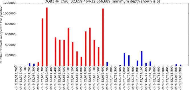
4.2 Coverage plot forHLA-DQB1. . . 40

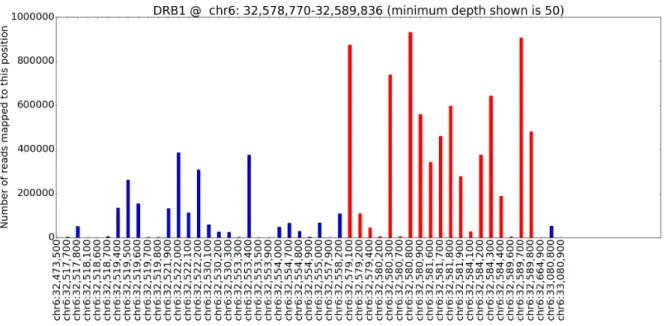
4.3 Coverage plot forHLA-DRB1. . . 41

4.4 Coverage plot forHLA-A. . . 41

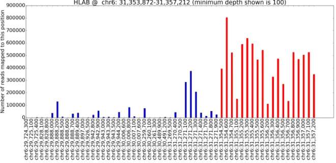
4.5 Coverage plot forHLA-B. . . 42

(9)

LIST OF FIGURES

4.7 File sizes of BAM files used in our training set before and after filtering. The files are ordered in ascending order by their file size before filtering. The file sizes are in MiB and we use logarithmic scale. . . 43 4.8 The weighted average impute INFO score for the two threshold qualities:

The mismatch quality thresholdρ(blue) and the clipping thresholdτ (red). Note that the axes do not start at zero. . . 46 4.9 The weighted average impute INFO score for different minimum sequence

length. Note that the axes do not start at zero. The results show that changing the minimum sequence length is insignificant. . . 48 4.10 The weighted average impute INFO score for different values of the zygosity

(10)

(11)

List of Tables

1.1 The number of alleles for the six most important HLA genes known to the IMGT/HLA database. . . 5

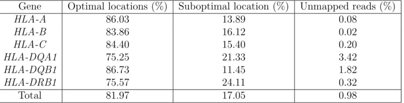
4.1 The fraction of reads mapped to the optimal locations, suboptimal loca-tions, and no locations of the human genome reference. . . 39 4.2 Checking for bias introduction our filtered BAM files. Only the most

com-mon Icelandic alleles were used in this analysis. Larger numbers mean greater unwanted bias. . . 45 4.3 Number of individuals in each verification dataset. . . 50 4.4 Gyper’s 2 digit genotype call accuracy compared to deCODE’s verification

data. . . 51 4.5 Gyper’s 4 digit genotype call accuracy compared to deCODE’s verification

data. . . 51 4.6 Gyper’s 2 digit impute accuracy compared to deCODE’s verification data. 52 4.7 Gyper’s 4 digit impute accuracy compared to deCODE’s verification data. 52 4.8 Gyper’s 2 digit exome accuracy compared to Erlich et al. [2011]. . . 53 4.9 Gyper’s 4 digit exome accuracy compared to Erlich et al. [2011]. . . 53 4.10 Gyper’s 2 digit low coverage WGS accuracy compared to Erlich et al. [2011]. 53 4.11 Gyper’s 4 digit low coverage WGS accuracy compared to Erlich et al. [2011]. 53 4.12 OptiType’s 4 digit call accuracy on 1000 Genomes’ exon dataset compared

to Erlich et al. [2011]. . . 54 4.13 OptiType’s 4 digit WGS genotype calling accuracy compared to Erlich

(12)

LIST OF TABLES

A1 Gyper’s called HLA-A genotype on 1000 Genomes’ exome dataset com-pared to Erlich et al. [2011]. . . 59 A2 Gyper’s called HLA-B genotype on 1000 Genomes’ exome dataset

com-pared to Erlich et al. [2011]. . . 63 A3 Gyper’s called HLA-C genotype on 1000 Genomes’ exome dataset

com-pared to Erlich et al. [2011]. . . 67

B1 Gyper’s called HLA-A genotype on 1000 Genomes’ low coverage WGS dataset compared to Erlich et al. [2011]. . . 71 B2 Gyper’s called HLA-B genotype on 1000 Genomes’ low coverage WGS

dataset compared to Erlich et al. [2011]. . . 72 B3 Gyper’s called HLA-C genotype on 1000 Genomes’ low coverage WGS

(13)

Acknowledgments

First, I would like to thank my father, Eggert Guðjónsson, and mother, Bryndís Helga Hannesdóttir. Not only have they passed down to me my splendid genes, but they have also showed me love and support all my life which I am deeply grateful for. It is truly privileged to have them as my parents. I am also greatly thankful my girlfriend and soulmate Bryndís Tryggvadóttir, her support for me, even in the toughest of times you have helped me believe in myself.

I also want to thank University of Iceland and their teachers for an amazing job of guiding me. It is seems absurd to get such a world class level of education while not needing to pile up student loans. The teachers at the university have really given me the strive for excellence and helped me achieve my dreams.

During the work of this thesis I’ve been completely stumped by how much trust and facility deCODE and its helpful employees have given me. Thank you everyone at deCODE who have given me this opportunity. A special thanks goes to my advisors, Bjarni V. Halldórsson and Páll Melsted, who have given me nothing but patience and constructive feedback. I hope to be able to work with you in the future.

(14)

(15)

Abstract

The major histocompatibility complex has an important role for the immune system in thousands of species. The human leukocyte antigen (HLA) is the human version of the complex and is located on the short arm of chromosome 6. Identifying an individual’s HLA genotype can give valuable information for medical applications. Several techniques already exist to HLA type an individual accurately, however they remain expensive and time consuming. Recently though, there has been a breakthrough in developing methods which use Next-Generation Sequencing (NGS) data for this purpose, due to its high availability. Using these methods we can genotype individuals using purely computation on sequencing data. However, these NGS methods remain somewhat time consuming, often requiring hours or days.

We introduce Gyper, a new open-source software which genotypes individuals for HLA using NGS data in a matter of seconds. Gyper’s speed is obtained by selecting a small subset of reads to consider and align them to the references in a partial order graph. Using Gyper we genotyped about 4,000 Icelander in deCODE’s dataset for the six major HLA genes. The resulting data was imputed for more than 150.000 Icelanders. Comparing those results with our verification data showed over 96% accuracy. Additionally we genotyped individuals from the 1000 Genomes project for the HLA class I genes and Gyper’s accuracy was always equal or higher than other HLA genotypers. These results show that Gyper can provide an impressively fast, yet reliable, genotyping results for a wide range of applications.

(16)

(17)

Ágrip

Major histocompatibility complex er hópur gena sem spilar lykilhlutverk í ónæmiskerfi þúsunda lífvera. Í manninum er hann kallaður human leukocyte antigen (HLA) og er staðsettur á styttri armi litnings 6. Vitneskja um hvaða genasamsætu einstaklingur hefur er mikilvægt fyrir svið læknisfræðinnar. Ýmsar leiðir eru til staðar sem geta til um tegund HLA genasamsætu einstaklings með hárri nákvæmni en þessar aðferðir eru dýrar og tímafrekar. Nýlega hafa margar aðferðir sprottið upp sem nota DNA raðgreiningargögn í sama tilgangi vegna mikils aðgengis að slíkum gögnum. Helsti kostur slíkra aðferða er að þær krefjast aðeins tölvu og DNA raðgreiningargagna. Galli þeirra er að þær eru tímafrekar, oft þarf klukkustundir eða jafnvel daga til að vinna úr gögnunum.

Við kynnum Gyper, nýjan opinn hugbúnað sem finnur HLA genasamsætu einstaklings með raðgreiningargögnum á aðeins nokkrum tugum sekúnda. Hraði Gyper fæst með því að skoða aðeins lítinn, en mikilvægan, hlut af raðgreiningargögnunum og bera saman við genasamsæturnar á hagkvæman hátt. Við notuðum Gyper til að finna genasamsætu um 4.000 Íslendinga á sex mikilvægum HLA genum. Með tengslaneti ályktuðum við HLA genasamsætur fyrir um 150.000 Íslendinga. Sannprófun sýndi að Gyper náði að tilgreina rétta genasamsætu í yfir 96% tilfella. Til að bera niðurstöður okkar saman við önnur forrit, þá fundum við einnig genasamsætur einstaklinga úr 1000 Genomes verkefninu. Í öllum tilfellum var nákvæmni Gyper sú sama eða hærri. Niðurstöður okkar sýna að Gyper nær að vera mjög hraðvirkur, en á sama tíma nákvæmur, í tilgreiningu sinni á genasamsætum einstaklinga fyrir HLA svæðið og á sér mikla notkunarmöguleika.

(18)

(19)

1 Introduction

1.1 Genetics

The flow of genetic information within a biological system was first explained in 1956 by Francis Crick [Crick, 1956]. His explanation is called the central dogma of molecular biology [Crick, 1970]. It explains how deoxyribonucleic acid (DNA) stores genetic data about every organism and how it can be transcripted to ribonucleic acid (RNA), and how RNA is translated to protein.

If one would compare the genetic structure of any two individuals of the same species you will find a few differences. These differences can be very small, such as polymorphism of only a single nucleotide (SNP), or much larger, such as duplication of whole chromo-somes (e.g. down’s syndrome). We can identify these differences and associate them with observed properties, such as behavior, morphology, and diseases. We call the observed properties phenotypes.

In 1953, James Watson and Francis Crick discovered the structure of the DNA. It is shaped like a double helix [Watson and Crick, 1953], where each helix has the opposite direction. On each helix the genetic information is stored in four different chemical bases: Adenine (A), cytosine (C), guanine (G), and thymine (T). The bases are interconnected with hydrogen bonds, where adenine bonds with thymine and guanine bonds with cytosine. Each of the connected bases form a base pair.

Genes are made up of hundreds to tens of thousands of base pairs acting as instructions to make biological molecules called proteins. The genes can acquire mutations in their DNA sequence which results in different variants of the same gene, called alleles. Different alleles can either encode for the same protein, different versions of the protein, or they might even be unable to encode for the protein at all.

The coding sequence of a gene is the region which is translated to protein. Humans have eukaryotic cells, which are cells with a nucleus containing the DNA. In eukaryotic cells the coding sequence is not continuous, it is split among several parts called exons. The exons are separated by introns. On either end of a gene there is an untranslated region which marks the beginning and end of the RNA reading frame. A polymerase transcribes the DNA into a RNA and splices the exon sequences. There are also untranslated regions on each end of the RNA. Finally, protein is created by translating the RNA. Figure 1.1

(20)

1 Introduction

illustrates the process for an eukaryotic gene with three exons.

Figure 1.1: The flow of information within an eukaryotic cell system. The coding sequence for the proteins are the red, green, and blue regions. Exons are spliced together to form RNA which is translated to protein.

1.2 The human genome

The human genome contains more than three billion base pairs which are stored on 22 pairs of chromosomes plus a single pair of sex chromosomes, hence 46 chromosomes total. In every pair of chromosomes, one came from the father and one from the mother. In humans there estimated to be 20,000-25,000 protein-encoding genes [Consortium, 2004]. Genes, that have a similar function, are said to be in the same gene family.

An approximate assembly of the human genome has been created and is called the human reference genome. One such assembly is released by the Genome Reference Consortium (GRC). Its most recent release is called GRCh38p4 (build 38, patch 4).

(21)

1.3 Genotyping

Genome Browser. They provide a good way to view and search the genome with various useful information, such as the location of genes and genetic variations found in the reference [Kent et al., 2002].

One of the main use cases of the human reference genome is using it in a local sequencing alignment. In such alignments DNA sequences, which are sampled from an individual, are aligned to the human reference genome. If the sequence can be aligned to the reference it is said to be mapped to that location. Otherwise, if the sequence does not align to the reference anywhere, the sequence is unmapped. Aligning sequences this way is computationally much easier than doing a whole-genome assembly of the individual. A commonly used local alignment tool is called BWA [Li and Durbin, 2009].

1.3 Genotyping

Genotype is the combination of individual’s two alleles. The act of estimating the genotype is called genotyping. In the field of bioinformatics, one major topic is called genome-wide association studies for humans. In these studies the human genotypes are associated with diseases and other phenotypes. Much of deCODE’s current work is performing association studies on the Icelandic population.

A wide range of genotyping methods exist, each with their pros and cons. Many methods are expensive, time consuming, and require advanced laboratory instruments. Another cheaper option is to use DNA sequencing data. GATK [McKenna et al., 2010] is an example of a generic DNA sequencing data genotyper. In summary, GATK extracts aligned sequences that were mapped to a certain location of the genome to predict the genotype of an individual. For most genes GATK’s predictions are accurate. However, highly variable genes often cause problems because the human reference genome is unable to represent them well. Examples of such genes are the ones in human leukocyte antigen (HLA) gene family.

1.4 The HLA gene family

The HLA gene family contains over 200 known genes in three different classes: I, II, and III. It is the human version of the major histocompatibility complex (MHC) and is located on the short arm of chromosome 6. In class I there are three main genes: HLA-A,

HLA-B, and HLA-C. The proteins produced from these genes are on the surface of most cells. These proteins are bound to protein chains called peptides that have been exported from within the cell. The proteins from genes in HLA class I display these peptides to the immune system and if the immune system recognizes the peptides as foreign it can react to it, such as triggering the infected cell to self destruct. In HLA class II there

(22)

1 Introduction

are six main genes: HLA-DPA1, HLA-DPB1, HLA-DQA1, HLA-DQB1, HLA-DRA, and

HLA-DRB1.

The HLA allele sequences are available in the IMGT/HLA database [Robinson et al., 2015]. As of release 3.21.1, August 2015, there are more than 13,000 known HLA alleles and increasing fast. With such a high number of alleles, genotyping is a very tough challenge.

Previously, certain HLA genotypes have been associated with diseases. Such as type I diabetes [Kikuoka et al., 2001] and celiac disease [Kaukinen et al., 2002], which are both autoimmune diseases. In another recent study some HLA class II alleles have been associated with multiple sclerosis (MS) disease [Moutsianas et al., 2015]. Furthermore, many medical operations depend heavily on matching HLA genotypes between a patient and its donor, such as bone marrow transplantation [Hansen et al., 1980], and umbilical cord blood stem cell transplantation [Gluckman et al., 1999]. The best outcome of such transplants are produced when the donor is a sibling which is HLA identical to the patient. Unfortunately though, usually no such donor is available because there is only 25% chance that two siblings receive the same alleles from their parents. In these cases a transplant from a well-matched unrelated donor is required and most often has acceptable results [Beatty et al., 1985].

In recent years many new methods have been created to use sequencing data to genotype HLA. Such methods have reduced the cost of genotyping and require nothing but a com-puter and sequencing data. Currently one of the most promising HLA genotyper using sequencing data is OptiType [Szolek et al., 2014]. OptiType genotypes for the three main class I genes using an integer linear programming (ILP) algorithm. Its results show good accuracy. However, this method is still rather time consuming, requiring hours or days to compute.

1.5 Gyper

Gyper is a novel open-source genotyper which uses sequencing data to genotype indi-viduals. The motivation behind Gyper is to create a genotyper which genotypes highly variable genes in an accurate and fast manner. It uses aligned DNA sequencing data. The name Gyper is an abbreviation of Graph genotYPER. In this initial release Gyper supports six HLA genes. They are the three main class I genes and three class II genes:

HLA-DQA1,HLA-DQB1, and HLA-DRB1. Overall these six genes account for 12,534 al-leles or 93.5% of all known HLA alal-leles (Table 1.1). This means that number of genotypes is enormous. The HLA-B gene has almost eight million allele combinations possible. The speed is achieved by storing the allele references in a partial order graph (POG) and align only relevant reads to it. A partial order graph is a directed acyclic graph made up of nodes (vertices) and edges. Each node stores a single DNA base while the edges contain

(23)

1.5 Gyper

Table 1.1: The number of alleles for the six most important HLA genes known to the IMGT/HLA database.

Gene HLA-A HLA-B HLA-C HLA-DQA1 HLA-DQB1 HLA-DRB1

#Alleles 3,192 3,977 2,740 54 807 1,764

information about which reference allele traverses through that edge. We make use of the fact that sequencing data is usually stored aligned and indexed, meaning we can quickly get reads that have been mapped to certain locations of the genome. Considering only a small subset of reads will vastly improve the speed of the genotyping, but has a risk of not taking all relevant reads into account and therefore missing potentially valuable information. We estimate the genotype of an individual by counting how many reads can be aligned to each allele reference. Figure 1.2 shows an overview of Gyper’s pipeline. Two alleles need to be chosen, because we each have two chromosomes. If an individual has the same allele on both chromosomes, it is said to be homozygous for that gene otherwise it is heterozygous. One key challenge we faced was to determine this zygosity. Our method takes into account that reads from sequencing machines will often contain er-rors. For each base these machines estimate the likelihood of an error. We crop reads with low quality ends to reduce the number of errors in the data. Also, we allow mismatches in reads if that base is very likely to contain an error.

Gyper has several parameters that were optmized using a training dataset. The training dataset was gathered from about 4,000 Icelandic people. After training, we verified Gyper using both a verification dataset from deCODE and a widely used verification dataset for individuals in the 1000 Genomes project.

(24)

1 Introduction

Figure 1.2: Overview of Gyper’s genotyping pipeline. An individual is sampled and sequenced. The sequenced reads are aligned to the human reference genome. The HLA allele references are fetched from an external database. A partial order graph is created which stores all the alleles in a single graph for each gene. Finally, we align the sequenced reads to the graph and genotype the individual.

(25)

2 Background

2.1 Next-generation sequencing

Over the last several decades, many different sequencing methods have been developed. These methods determine the order of the nucleotide bases of a small DNA fragment. One widely used method, including at deCODE, is called next-generation sequencing (NGS). The machinery used is produced by Illumina which uses a synthetic approach to sequence individuals [Bentley et al., 2008]. Here we will describe the process used by those machines.

First, a sample of DNA is obtained and labeled from an individual (e.g. blood). Then, the DNA is randomly sheared into fragments of various length. The average fragment length can be set to different values but in deCODE’s dataset this length is typically around 500 bases and is almost always smaller than 1000 bases. To each end of the fragments the four types of bases are added in the mixture, each fluorescently labeled with a different color and attached with a blocking group.

Figure 2.1: A read pair. The two reads are read from one end of each fragment strands in opposite direction.

The four bases then compete for being the next base on the template DNA strand that is being sequenced. When one base has been attached all other non-incorporated molecules are washed away. After each synthesis, a photograph of the incorporated base is taken. For each base the likelihood of an error is estimated. The blocking group is then removed using a chemical process. This process is repeated until we have sequenced a certain number of read pairs.

(26)

2 Background

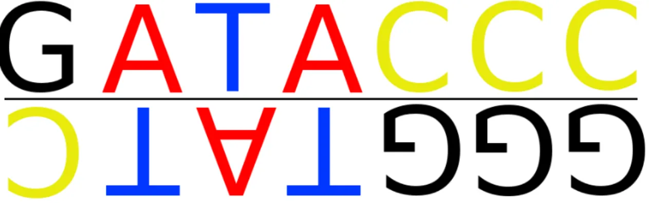
The reads of a read pair have different directions (Figure 2.1). On each end of a DNA strand there can either be a three-prime (3’) or a five-prime (5’). The direction of a read can either be from 3’ to 5’ or from 5’ to 3’. Also, we have an idea of the length between the two reads because they will both start on each end of the fragment. Both reads are reading the same chromosome, but different chromosome strands. Recall that A complements with T, and C with G. That means one strand will be the reverse of the other with A changed to T, T changed to A, C changed to G, and G changed to C. (Figure 2.2). One string is said to be the reverse complement of the other.

Figure 2.2: Two chromosome strands. A is always bonded with T and C is bonded with G. The reverse complementary of the sequence GATACCC isGGGTATC.

The total number of read pairs can vary, but generally it is aimed to have 30x coverage or more. The coverage is the average number of times each base pair is sequenced. Having a too low coverage means multiple locations are likely to be not covered by any reads. Since we are adding a single base in each step the most common error we might expect are mismatches, it is highly unlikely that we get errors in the form in insertions or deletions. Insertion is when an extra DNA base is added to the read by mistake and a deletion is when a base is mistakenly not read by the sequencer.

What distinguishes this method is that it is fast and cheap but the reads will be short, generally between 75 and 150 bases. In deCODE the read lengths used are 100, 120, or 150 base pairs. With today’s Illumina sequencing machines we can produce hundreds or thousands of sequences concurrently. In 2010, the cost of sequencing one million bases ranged from $0.05 to $0.15 USD and the required time is up to 11 days [Vliet, 2010]. In January 2014, Illumina released a sequencing machine capable of sequencing an individual for less then $1,000 with 30x coverage or about $0.01 per one million bases in three days [Hayden, 2014].

Each sequence is an extremely small fraction of the human genome and we have no information if our read contains any mistakes or where the read was located, only that it was on some random chromosome at some random location. We can never even be sure that all bases are included in our reads, some locations might still be completely missing. Assembling these reads is a process called whole-genome assembly and it is a very difficult problem.

(27)

2.2 Phred score

The problem can be looked at like this: We have many identical jigsaw puzzles cut in various ways. We remove a bunch of puzzles and also bend some of them around so they will not fit anymore and then try to solve the puzzle. To make the problem easier we can use a human reference genome. This can be thought as another very similar completed jigsaw puzzle. The idea is to compare the pieces we have with the completed puzzle to get a better idea where they can fit, changing the problem to an alignment problem. This task is still very computationally heavy and involves a lot of guessing. It is especially tricky for locations of the genome where variability is high, such as the HLA region. Moreover, there are many regions with high similarity to the HLA genes, which makes the task even harder.

2.2 Phred score

Phred quality score is a scaled quality score given to each base pair of a read. It is a commonly used in sequencing technology. It measures the probability of sequencing errors of each base pair in a read. The Phred qualityQis the log value of the probability of sequencing errors P(e) calculated using the formula:

Q=−10 log₁₀(P(e)) (2.1) For example, if the probability of error is 1% (i.e. 99% accuracy) then the quality score given is 20. Solving forP(e) we get

P(e) = 10−Q/10 (2.2)

The quality Q from Illumina machines range from 0 to 41 and are represented as an ASCII character c [Johnson, 2013]. The conversion from Q to c can be done by adding 33 to Q and convert the bits from that number to an ASCII character. Character 33 in the ASCII table is ‘!’ which is the lowest possible quality. Additionally, it is the first printable character in the table if we exclude the white space character ‘ ’. Using the lowest possible quality is never really done though, as it means there is 100% probability of an error. The highest quality character possible for Illumina machines is ‘J’, the 74th character in the ASCII table used for a quality score of 41. Using equation 2.2 it equals 0.00794% probability of an error. The quality values are stored as ASCII characters for space efficiency. For example, if the quality value 41 was stored as the string ‘41’ we would need two bytes instead of one.

(28)

2 Background

2.3 Data formats

2.3.1 FASTA format

The FASTA format is a common format for storing both nucleotide and amino acid sequences. It was created by William Pearson and was used in his program with the same name. Since then it has become the industry standard in bioinformatics for raw sequencing data [Pearson and Lipman, 1988]. It has a wide range of use cases. Frequently, it is used to store sequenced reads or even the whole human genome. Pearson did not have any particular specifications for the format, but here we will discuss how it is most commonly used. >chr6_7500001-7500350 GGTATGCCTGTATATACAAATGTTCCAGAATCTGAAAAAATCCAAAGTTC AAAACATATCTAGTCCCAGGCATTTCAGATAAGGGATACTCTGTGTGTGT GTGTGTGTTTGTGTGTGTGTGTGTGTGTGTGTGTATGAATTTTGAGAGTG TTGTTTATTTTTATTTTGTAAATACAAGGTCTTGCTCTGTCACCCAGGCT GGAGATCAGTAGCATGATCACATTTCACTGCTGCTTTGAACTCTGACTCA AGGAATTCTCCCTCCTACCTCAGCCTCCCAAGTAGGTAGGACTCCCAAGT AGGTGGCGTACACCACCATGCCTGGCTAATTTATTTTATTTTTTCTAAAG

Figure 2.3: Example FASTA file entry for a sequence from the human reference genome. Here the sequence ID is chr6_7500001-7500350 meaning the sequence is from chromosome 6 and is showing bases located at 7500001 to 7500350. The sequence description is omitted. Following the header is the sequencing data split by 50 characters per line.

Each entry in a FASTA file has a single header line which always starts with the greater-than symbol ‘>’. It is followed by the sequence ID that cannot contain any white spaces. Optionally, the sequence ID is then followed by a white space and then a description of the sequence. The sequence ID often contains some useful information about the sequence. In the next line after each header is its sequencing data. There, each nucleotide is stored as a single character. For example we store the DNA chemical bases adenine, guanine, cytosine, and thymine as A, G, C, and T respectively. For easier readability, it is rec-ommended that each line will not exceed 80 characters, thus sequences longer than 80 characters need to be split into multiple lines [Genestudio, 2015]. However, since headers are only allowed to be in a single line they can break the 80 character restriction. In ad-dition, every line has the same length except perhaps the last one. This restriction makes it possible for FASTA readers to be able to know where the last location of the newline character can be, thus improving reading performances slightly. The sequence continues until the next header line or the end-of-file (EOF) file descriptor has been reached. An example entry in a FASTA file is shown in figure 2.3.

(29)

2.3 Data formats

Files using the FASTA format have the.faor.fasta extensions. The FASTA format has some extensions, such as the FASTQ format which also includes a quality score for each base. FASTQ files have the.fq or .fastq extensions. To make searches in big FASTA files faster the files are often indexed and saved in FASTA index files. They have the extensions .fa.fai or .fasta.fai. For example, SAMTools [Li, 2011] indexes FASTA files.

2.3.2 SAM and BAM format

For storing aligned reads the sequence alignment/map (SAM) format is often used. The SAM format has two sections: An optional header section and an alignment section. Lines in the header section always start with the character ‘@’. In the alignment section each sequence is stored in one line. In each line there are 11 TAB delimited mandatory fields. If these fields are unavailable they must still be defined with the values ‘0’ if the field contains a number or ‘*’ if it contains a string.

There are also optional fields that can be used by storing key-value pairs in the format of TAG:TYPE:VALUE where tag is the key. Many tags are predefined such as the RG tag which stores the read group of the sequence.

A companion format to SAM is the binary alignment/map (BAM), it stores the exactly same data as SAM but is compressed using the BGZF library and encoded to binary. The compression is focused on performance rather than high compression [Li et al., 2009]. SAM and BAM files are stored in .sam and .bam files, respectively. Most commonly they are used in storing next-generation read alignments. The SAM specifications are constantly being updated by the SAM/BAM format specification working group which is a part of the SAMTools project group. SAMTools is a software package and library that can work with SAM and BAM files. They provide many tools for SAM/BAM files such as conversion from and to other formats, filtering, compression, decompression, sorting, indexing, merging files, and more [Li, 2011].

CRAM is another companion format to SAM. It allows for a highly efficient reference-based compression of SAM files reference-based on Fritz et al. [2011]. The files are stored with a .cram extension. The reference-based compression algorithm is capable of storing the data in smaller files than BAM does.

2.3.3 VCF

The variant call format (VCF) is a format to store genetic variation data. FASTA files work very well when displaying sequences with no variations, such as the human genome reference, but often it is necessary to be able to view variations of a reference. The VCF

(30)

2 Background

format tries to do this in an efficient manner. It shares many similarities with SAM/BAM files. The variations supported include single nucleotide polymorphism (SNP), insertions, deletions, and structural variants. One reference genome is used and then variations are stored as alternative sequence to the reference.

Files using the VCF format are usually saved with the .vcf extension. Similar to SAM/BAM files VCF files have a header section and data section. Lines in the header section start with the character ‘#’ or ‘##’ depending on if the line stores data columns or meta information, respectively. The meta information is stored as key=value pairs. VCF files have eight mandatory columns which can be omitted with a ‘.’ character. They are usually stored compressed using the BGZF library [Danecek et al., 2011].

2.4 The HLA reference alleles format

The HLA reference alleles are represented using a specific naming format. First the gene family is be defined, followed by the gene name. The family is HLA for the six genes supported by Gyper. Each type, subtype, synonymous substitution and non-coding substitution will then have an unique set of 2 digit numbers. Sometimes the name will have a suffix character that represents a change in the protein expression. (Figure 2.4)

Figure 2.4: An example of a reference allele format.

Every allele has at least 4 digits so the family, gene, type, and subtype fields are manda-tory. Beyond that, the fields are only used when needed. Sometimes there are more than a hundred different subtypes. In these cases the subtypes have 3 digits. However, alleles with 3 digit subtypes do not have increased resolution. For example the allele

HLA-A*02:102 is considered having a 4 digit resolution, not 5.

Different types and subtypes mean that the two alleles will produce different proteins. This means the exon DNA sequences of the alleles are different. However, it is possible that the exon DNA sequences are not the same but they will still both translate to synonymous proteins. These substitutions are called synonymous substitutions because

(31)

2.5 Current DNA sequencing genotypers

they do not affect the translated protein. Sequences that differ only in exon sequences but not in translated proteins are distinguished by the 6 digit resolutions. Finally, the 8 digit resolution will distinguish substitutions in the non-coding region, that is variations of introns.

Genotyping techniques that use HLA proteins are only capable of 4 digit resolution typing. For most applications we are only interested in genotyping for different proteins, therefore 4 digit resolution is sufficient. By using DNA sequencing data we are capable of genotyping with up to 8 digit resolution.

2.5 Current DNA sequencing genotypers

Before Gyper, other programs have been created with same purpose of genotyping using sequencing data. Gyper is highly influenced by one named OptiType [Szolek et al., 2014]. OptiType genotypes using an integer linear programming (ILP) algorithm. They tested their algorithm on a broad range of sequencing data: Whole genome sequencing data, RNA data, and exome sequencing data - which only contains exon data. Their results are very good, their comparison to verification data are showing 97% accuracy with 4 digit resolution. In our study we compared Gyper to OptiType, as their algorithm has shown to have better or equally good accuracy in comparison to other HLA genotyping programs.

HLAminer [Warren et al., 2012] is a widely used program for genotyping with sequencing data. Their focus is on Illumina shotgun sequencing data. In summary, their method involves doing a HLA assembly using a tool called TASR. Then comparing the assembly to the reference alleles using a hash table filled with every 15-nucleotide word, or 15-mers, encountered. The program genotypes very quickly but in comparison to the other tools their accuracy is not very high. For example, their accuracy compared to OptiType was reported to be about 15% lower [Szolek et al., 2014].

ATHLATES [Liu et al., 2013] is another tool that uses HLA assembly to genotype. Their methods rely on accurate recovery of the exon sequences via the assembly. It uses many of the ideas behind HLAminer but improves them and deliver a much better results. Their reported accuracy 74 out of 75 allelic pairs or about 99% overall accuracy. OptiType compared themselves with ATHLATES and both programs showed a similar accuracy. However, the sample size was very low, only 3 genes typed for 11 individuals [Szolek et al., 2014].

Recently, a HLA genotyper was created by Major et al. [2013]. It filters the DNA se-quencing data and then matches those reads to the exon sequences of the HLA alleles. In the alignment they discard reads with too many mismatches or any indels. Their method achieved a good HLA call accuracy of 94.2% for an exome dataset. However, on the same dataset OptiType achieved even better results.

(32)

(33)

3 Methods

Figure 3.1: Modified version of Gyper’s pipeline (Figure 1.2). The scope of the three main steps are highlighted.

Our method has three main steps:

• Preprocess the data (Section 3.1).

• Create the partial order graph (Section 3.2).

• Align reads to the partial order graph to genotype the individual (Section 3.3).

Figure 3.1 declares the scopes of these steps. The preprocessing step is released as a separate contribution. Gyper’s scope only covers the creation of partial order graph and alignment to it. In section 3.4 we discuss the different adjustable parameters Gyper has and in section 3.5 how we train these parameters. Finally, in section 3.6 we will touch on the implementation and availability of Gyper.

(34)

3 Methods

3.1 Preprocessing the data

The preprocessing is released separately from Gyper because it depends on external li-braries, which we did not want to add as dependencies. Furthermore, the processes in this step are exclusive to the HLA genes.

3.1.1 Fetching the HLA reference alleles

The HLA reference alleles were fetched from the IMGT/HLA database [Robinson et al., 2015]. The database is released in various formats: FASTA, flat files, MSF, PIR, and XML. We used the XML database.

To reduce the size of the database, there are few alleles that work as a template for other alleles. Template alleles have information about its full sequence with all features (exons, introns and untranslated regions) and references itself as a template. Each non-template allele only specifies features that differ from its template allele. This structure made it tedious to fetch the allele sequences for all non-template alleles manually.

To simplify the process we created a XML wrapper which depends on RapidXML, a fast XML DOM parser library in C++ [Kalicinski, 2015]. Our wrapper fetches features of all alleles and outputs them in a FASTA file. Figure 3.2 shows an example output.

In the output FASTA files the first two letters of the header is the feature identification code. The allowed codes are 5P, P3, E[0−9], and I[0−9]. Features with 5P and P3 are the untranslated regions closer to the 5’ and 3’ strand ends, respectively. E[0−9] represents exons 0 through 9 andI[0−9] introns 0 through 9. The number of exons differ among genes.

>E5_HLA-DQB1*03:02:01 GACCTCAAGGGCCTCCACCAGCAG >I5_HLA-DQB1*03:02:01

GTGATATTTCAGCCATGAGCCAGTGTGGGGGGGCACAGGTGTAAGAGGGAAGA...

Figure 3.2: IMGT/HLA XML wrapper example output.

The direction of the reference alleles are from 5’ to 3’. To get the full sequence of the allele the features should be concatenated in the following order: 5P, E1, I1, E2, ..., EN, P3. Where N is the total number of exons for a given gene.

(35)

3.1 Preprocessing the data

3.1.2 Regions with relevant reads

The HLA gene cluster is only a very small part of the whole human genome, and thus only a very small portion of the sequenced reads is relevant to HLA genotyping. We could expect a huge reduction in the time taken to perform the genotyping, if we would only need to consider those reads. However, finding the relevant reads is difficult.

One solution is to use every read pair that has been aligned to the gene’s position on the reference genome, such as GATK does [McKenna et al., 2010]. Our concern is that such an approach is unable to have accurate results for the HLA region due to its high variability. Reads from the HLA region are often misaligned since the human reference genome cannot represent those regions well.

Another solution would be to take every sequenced read into account, such as OptiType does [Szolek et al., 2014]. Their method involves considering every read pair by first mapping them to all HLA alleles, and then use all the mapped reads to genotype the individual. Their assumption is that the true genotype can explain the most reads. But we have two concerns. First, taking every read into account takes a very long time, hours or days using whole genome sequencing (WGS) data. Only a very small portion of the reads are even relevant to the genotyper. Second, using reads that are mapped elsewhere risks biasing the results. For example if a sequence outside the HLA is very similar to one or more alleles but not all, those particular alleles will be biased to score higher than the other alleles. This results in the genotyper predicting the alleles most similar to the reference too often.

Regions of interest

We propose a different method. Our method makes use of the fact the reads are usually stored aligned in alignment files (SAM/BAM files). All read pairs belong in one of three categories:

• Both reads are mapped to the reference genome at locations l1 and l2, and usually we expect them to be relatively close to each other, we assume 0 ≤ |l2−l1| ≤850.

• One read is unmapped, but the other read in the pair is mapped to location l. By convention, both reads are marked to be located at l.

• Both reads are unmapped. The reads are both marked as unmapped.

Our goal is to find regions of the genome which are likely to have HLA relevant reads mapped to them. The following three steps explain our process:

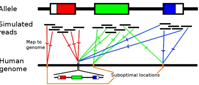
(1) Simulate reads that overlap the alleles’ exons.

(36)

3 Methods

(3) Check where the simulated reads map.

Figure 3.3 shows the process for a single allele. The aligner will map to a correct location, a suboptimal location outside HLA, or not map the read to any position of the genome. We are only interested in reads overlapping the exons, since the exons determine the first 6 digits of the HLA genotype. All aligned positions are extracted and used as the regions of interest.

When genotyping, we only use reads located inside the regions of interest. We hope that filtering the data this way will decrease the overall computational time of the genotyping without decreasing its accuracy significantly.

Figure 3.3: Flow chart for finding relevant positions of the human genome using one allele. Reads overlapping the exons are simulated and mapped to the human reference genome.

Algorithm

Algorithm 1 shows the pseudo code behind this technique. For step (1) we gather all sequences for both exons and introns from our fetched reference HLA alleles. As we are only interested in the exons, we look for reads overlapping the exons completely or partly. In our case we simulated reads of length 100 base pairs so we used 100 bases from each intron. If, for example, the exon is of length 20 base pairs, the complete sequence will be 100 intron base pairs, 20 exon base pairs, and then another 100 base pairs sequence for a total of 220 base pairs.

Reads are simulated using a read simulator called Mason, which is provided as part of the C++ library SeqAn [Döring et al., 2008, Holtgrewe, 2010]. Mason simulates sequencing

(37)

data in a realistic manner, so some sequences will contain errors. Mason was run with the Illumina machine settings so the chance of a mismatch will be much higher than an insert or deletion.

Step (2) is by far the most computationally intensive step, requiring each simulated frag-ment to be mapped to the human reference genome. In this step we explicitly call the Burrows-Wheeler Aligner (BWA) to map the fragments [Li and Durbin, 2009]. The BWA-MEM algorithm was chosen for the task. Its output is a SAM file with our simulated reads aligned to the human reference genome. We discarded reads that the BWA could not align to the reference.

Steps (1) and (2) were implemented in a single C++ program. Step (3) requires sorting all mapped positions from the previous step and keeping them in two sorted lists, one for all the starting positions and one for all the end positions. The end position is required because sometimes BWA will only align a partial read. By looping through both lists we can know at any point what the coverage depth is. The coverage depth of a base is the number of reads that overlap that base.

The algorithm starts on the start position, and checks the coverage of each base until we have reached the final position. The first item in the starting position list is the start position, and the last item in the end position list is the final position. Most bases of the genome have no coverage depth, but we can always skip to the next item in the start position list when that occurs.

Checking for bias introduction

When extracting reads outside the HLA region we might be introducing a bias to the results for some of the HLA alleles. For example, if the suboptimal regions contains sequences which are very similar to some alleles, but not all. If that happens those alleles will have a biased score. We can correct for this bias by adding a parameter in Gyper which lowers the scores of the biased alleles.

To measure the bias we simulate read pairs from all suboptimal locations we found and use them in Gyper. We can then get an estimate of how often this event happened. Reads are simulated with Mason using Illumina settings with 3000x coverage depth. Results can be found in section 4.1.3.

3.1.3 Multiple sequence alignment

In section 3.1.1 we parsed all features of the HLA alleles. Aligning the sequences in a multiple sequence alignment (MSA) will be beneficial to the algorithm that creates the partial order graph for two reasons: First, all the sequences have the same length. Second,

(38)

3 Methods

Input : All reference alleles for each genotype (alleles), number of random fragments (n), and length of intron sequences to use (intronLength).

Output: All locations of the genome and their coverage depth, excluding all location with no depth.

1 exons ← Fetch all exons using our IMGT/HLA XML parser. ; Step 1 2 Add sequences from surrounding introns of up to length intronLengthon each end

of the exons.;

3 fragments ← Generate n random simulated reads fromexons.;

4 startPositions, endPositions ←Array with all zeros of length n ; Step 2

5 for i←0 to n−1 do

6 startPositions[i] ←Map(fragments[i]);

7 endPositions[i] ← startPositions[i] + Length(fragments[i])

8 end

9 startPositions ←Sort(startPositions) ; Step 3 10 endPositions ← Sort(endPositions);

11 location, depth ← Empty array; 12 i, j, k, d←0; 13 while k ≤ endPositions[n-1]do 14 if startPositions[i] ≤k then 15 i+ +; 16 d+ +; 17 continue 18 end 19 if endPositions[j] ≤k then 20 j+ +; 21 d− −; 22 continue 23 end 24 if d is 0then 25 k ←startPositions[i] 26 end 27 else 28 Add k tolocation; 29 Add d todepth; 30 k+ +; 31 end 32 end

Algorithm 1: Extracting regions from the genome which are likely to contain misaligned HLA reads. We do that by first simulate HLA reads, map them to the genome, and determine which locations they were mapped to.

(39)

most sequences will share a base, so we can use a single node to represent a base on most or all alleles.

MSA has been used before for this purpose, for example Dilthey et al. [2015]. We align the sequences by inserting gaps into the them. In the graph, gaps are represented by the absence of a node so adding gaps will not increase the number of nodes in the graph. In fact, by aligning the sequences we can often use fewer nodes to represent the sequences. So the MSA is effectively reducing the number of nodes required for the graph.

However, an optimal MSA is massive for this case. The worst case has close to 4,000 different sequences with an average length of over two thousand base pairs (N ≈4000, L >

2000). Optimal MSA has proven to be a NP-hard problem [Wang and Jiang, 1994] and with a complexity of O(LN). So an optimal MSA would take absurdly long time for our case and is not necessary. Approximate MSA is more appropriate. We use MUSCLE, which does an approximate MSA with high accuracy. The complexity of MUSCLE’s MSA algorithm isO(N3_L₊_{N L}2_{) [Edgar, 2004].}

Figure 3.4 shows an example of our data before and after the MSA. The input and output are both in FASTA format, and the output sometimes contains dashes which represent gaps. Specifically, these are sequences shown are the 4th intron for alleles HLA-C*15:02:01, HLA-C*16:01:01, and HLA-C*17:01:01:01. For clearer representation we have colored mismatches as red, and indels as green. For these three reference alleles,

HLA-C*15:02:01 and HLA-C*16:01:01 only have one base mismatch between them. Se-quencesHLA-C*16:01:01andHLA-C*17:01:01:01however, there are 2 bases mismatched and another 3 bases inserted into HLA-C*17:01:01:01.

(40)

3 Methods Input: >I4_HLA*15:02:01 GTAAGGAGGGGGATGAGGGGTCATGTGTCTTCTCAGGGAAAGCAGAAGTCCTGGAGCCCTTCAGCTGGGT CAGGGCTGAGGCTTGGGGGTCAGGGCCCCTCACCTTCCCCTCCTTTCCCAG >I4_HLA-C*16:01:01 GTAAGGAGGGGGATGAGGGGTCATGTGTCTTCTCAGGGAAAGCAGAAGTCCTGGAGCCCTTCAGCCGGGT CAGGGCTGAGGCTTGGGGGTCAGGGCCCCTCACCTTCCCCTCCTTTCCCAG >I4_HLA-C*17:01:01:01 GTAAGGAGGGGGATGAGGGGTCATGTGTCTTCTCAGGGAAAGCAGAAGTCCTTCTGGAGCCCTTCAGCCG GGTCAGGGCTGAGGCTTGGGTGTAAGGGCCCCTCACCTTCCCCTCCTTTCCCAG Output: >I4_HLA-C*15:02:01 GTAAGGAGGGGGATGAGGGGTCATGTGTCTTCTCAGGGAAAGCAGAAGTC---CTGGAGCCCTTCAGCTG GGTCAGGGCTGAGGCTTGGGGGTCAGGGCCCCTCACCTTCCCCTCCTTTCCCAG >I4_HLA-C*16:01:01 GTAAGGAGGGGGATGAGGGGTCATGTGTCTTCTCAGGGAAAGCAGAAGTC---CTGGAGCCCTTCAGCCG GGTCAGGGCTGAGGCTTGGGGGTCAGGGCCCCTCACCTTCCCCTCCTTTCCCAG >I4_HLA-C*17:01:01:01 GTAAGGAGGGGGATGAGGGGTCATGTGTCTTCTCAGGGAAAGCAGAAGTCCTTCTGGAGCCCTTCAGCCG GGTCAGGGCTGAGGCTTGGGTGTAAGGGCCCCTCACCTTCCCCTCCTTTCCCAG

Figure 3.4: Example input and output of our MSA. Bases colored green and red are indels (insertions or deletions) and mismatches, respectively.

(41)

3.2 Constructing a reference partial order graph

3.2 Constructing a reference partial order graph

Typically sequences are aligned to a single reference genome. For genes with high struc-tural and sequence diversity this can lead to poor characterization of such regions. To represent these genes, such as the HLA genes, we used a partial order graph (POG).

3.2.1 Graph implementation

In the POG we both store nodes (vertices) and directed edges. By doing a MSA we ensure that every feature has the same length. The features are added to the graph one by one. Each node has an integer that stores the level and a single DNA base value, that is A, T,

G, or C. We surround each feature with a node that has no DNA base.

The level corresponds to the location of that base in the sequence. No two nodes connected by a direct path can have the same level. If n1 and n2 are two connected nodes in the graph the edge will always be directed to the node with the higher level. This means that the last node of the graph, the one with no outgoing edges, has the highest level. The first node of the graph, the one with no incoming edges, has a level 0.

Each edge stores reference to both nodes it connects with. Furthermore, if the edge is inside an exon it also stores a bit string. The bit string has a length equal to the number of references used. The purpose of these bit strings will be discussed when we align sequences to the graph and genotype in section 3.3. When an edge is created all bits are initialized to 0 except for the one representing the exon that is being added.

When adding another sequence to the graph which shares a path with an earlier sequence, we flip the corresponding bit to 1. By storing it this way we never need more than ceil(r/8) bytes memory per edge, where r is the number of references used in the graph. If, for example, we had 1000 references and 10,000 edges we would only need 1.25 megabytes to store this information. Additionally, we only need to store it for exons. Algorithm 2 shows the pseudocode behind this method and figure 3.5 shows an example how it creates a graph for three exon sequences: GATA,-AT-, and CATA.

We add exons and introns sequences separately because edge creations are handled differ-ently, exons have a bit string while introns do not. There is high amount of missing and unreliable intron data in the IMGT/HLA database, compared to the exons. So instead of trying to reuse data from other introns we simply allow reads to align freely within the intron. With such free alignment there is no need for the bit strings, so they are omitted on introns.

(42)

3 Methods

Input : Fasta file with aligned sequences of some feature.

Output: Partial order graph we can use as a reference.

1 graph ← empty partial order graph;

2 sequences ← read sequences from Fasta file; 3 previous ← new node with level 0.;

4 endNode ← new node with level Length(sequences[0])+ 1.;

5 Add previous and endNode to graph.; 6 for sequence in sequences do

7 for pos in Length(sequence) do 8 if sequence[pos] is a gap then

9 continue;

10 end

11 node ← node with letter sequence[pos] and level pos+ 1.; 12 if node exists in graph then

13 next ← node;

14 if No edge exists from previous to next then

15 Add Edge between previous and next with bit pos flipped on.

16 end

17 else

18 Flip bit pos on for edge from previous tonext.

19 end

20 end

21 else

22 Add node tograph.;

23 Add Edge between previous and next with bit pos flipped on.

24 end

25 previous ← next;

26 end

27 if No edge exists between previous and endNode then

28 Add Edge between previous and endNode with bit pos flipped on.

29 end

30 else

31 Flip bit pos on for edge from previous tonext.

32 end

33 end

Algorithm 2: Creating a reference partial order graph for a single exon. Creating a graph for an intron is similar but then we do not store the bit string on edges, hence no need to create or modify them.

(43)

Levels

0 1 2 3 4 5

a)

b)

G

A

T

A

001

001 c)

G

A

T

A

001

011

001

010

010 d)

G

A

T

A

001

111

101

010

010 C

100

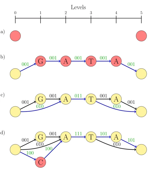
Figure 3.5: Create a partial order reference graph using three example exon sequences:

GATA,-AT-, andCATA. Blue edges show edges we traversed through, green labels represent changed or new labels on edges. Red and yellow nodes represent new and old nodes, respectively. a) Two nodes are created, initial node on level 0 and a final node on level

Length(sequences[0]) + 1, which is here 5. b) The sequence GATAis added to the graph. c) The sequence-AT-is added to the graph. Note that no new nodes need to be created, only edges. We change the bit string for the edge going from A to T so it includes this sequence. d) The sequence CATA is added to the graph. The new C node will be on the same level as the G node.

(44)

3 Methods

3.2.2 Extending the POG

Figure 3.6 shows how the partial order graph can be extended with three intron sequences:

TTA, -TA, and GTA. In our implementation we extend the graph by adding sequences connecting to the lowest level node. So when creating a graph for the HLA genes we add features in reversed order: First the 3’ untranslated end of the allele, then the last exon, then the last intron, and so on until we have added the 5’ untranslated region.

The nodes connecting the features are always free to traverse through so they do not need to store any DNA base. We keep track of the level of these nodes. When we are aligning to the graph we can check the level of the node we are aligning to. So at any point in the alignment, we know if we are aligning to an exon or an intron.

(45)

G

A

T

A

001

111

101

010

010 C

100

100 T

T

G

A

Figure 3.6: Extended graph from figure 3.5. Here we have added three intron references to the graph. We use the previous initial node as a final node for the new extension. The red nodes are the new intron nodes. The intron sequences we have added are: TTA, GTA, and -TA. Note that the edges on the new nodes do not store a bit string like the other exon nodes.

(46)

3 Methods

3.3 Aligning sequences to the POG

When aligning sequences to our graph the goal is to determine which pair of alleles can explain the most reads. Our assumption is that this pair of alleles is the individual’s true allele pair.

We have a backtracker which both to keeps track of the read’s path through the graph. The match is simply an array of boolean values equal to the length of the read. This array initially has all bits set to 0, which are flipped if a match is found. The backtracker also stores which node is the previous node of the match, so we know how the match traversed through the graph. The size of the two arrays are the same as the length of the read we are aligning. In our alignment we are free to start anywhere and end anywhere, it is a semi-global alignment where both of the ends of the references are free. Generally we would need to have our two arrays equal to the length of the read plus one, but since we can start anywhere the top boolean will always be true so there is no need to store that.

Since the graph is acyclic we can always find topological sorting of the nodes, meaning if there is a node n1 which depends on the results of node n2, n2 will never depend on n1 or any of n1’s dependencies. Also there is one, and only one, node that does not depend on any other nodes. That node is the first node in our topological sort.

3.3.1 Algorithm

We use a dynamic programming algorithm to align sequences to the graph as shown in algorithm 3. Our algorithm requires O(nm) time in the worst case, where n is the number of edges and m is the length of the sequence. It visits every edge on the graph and compares the DNA base of the sequence to the target node.

When traversing through the graph it is always guaranteed that we have already calculated the current node’s dependencies. When matches are found we only need to change a boolean value in the array and store a reference to the previous node. The aligner can find a list of nodes where the sequence was matched, because the sequence can be aligned to more than one location. If we align both reads in a read pair to a location that is very far from each other we discard that read pair.

The highest distance between reads allowed is arbitrarily chosen to be 800 base pairs. If the read is aligned to multiple locations we need to choose the best one to use. We chose the best distance between two reads to be 350 base pairs. These two values were estimated from the 99.99% highest and the most common insert sizes of deCODE’s BAM files, respectively.

(47)

3.3 Aligning sequences to the POG

matches the read to nodes 4 (A), 5 (no base), 7 (C), 8 (A), and 9 (T). Here, a reference to the 9th node will be the only node in the output list. Then, when the alignment has finished, we backtrack from that node only. Backtracking has a complexity of O(m) in the worst case.

3.3.2 Backtracking

The backtracking algorithm uses the backtracker to determine which reference alleles can explain the aligned read. It picks a node from the alignment algorithm and starts back-tracking there. Initially it has a bit string of length equal to the amount of reference alleles used with all bits flipped to 1. Then, as the backtracking algorithm travels backwards through the graph it will perform a bitwiseANDoperation for every edge with a bit string. That is, if we are traversing inside an exon we will perform theAND operation.

What we end with is a bit string whose bits are only flipped on if the read followed the corresponding reference allele exactly. In other words we say that those reference allele explain the read. If however we are traversing through an intron we do not know which reference allele created that edge on the graph, we would rather say that any reference can explain the read for the reasons we discussed before.

Continuing with the previous example (Figure 3.6) the backtracking of the sequenceACAT

would generate the following calculations:

111AND111AND100AND100 = 100

The convention when using bit string is to say they the rightmost bit is the first one. So the bit string 100 means that only the third reference explains the read. The exon of the third reference wasCATAwhichACAToverlaps. ACATdoes not overlap the other two exons. If however we aligned the readTTA, the read maps to nodes 1, 3, and 4. Since these nodes are not connected to an edge with a bit string we will not require anyANDoperations and simply have the bit string:

111

(48)

3 Methods

Input : A sequenced read from an individual who is being genotyped for gene gene.

Output:backtracker we can use to find all references that explain the read and an array of nodes where alignments end at.

1 graph ← a partial order graph for gene.; 2 order ← TopologicalSort(graph);

3 backtracker ← array for each node in graph storing both match (true orfalse)

and previousNode.;

4 nodes ← empty array. 5 for source in order do

6 for edge in edges directed from source do 7 target ← edge’s target.;

8 if target stores dna then

9 if read[0] == target.dna then

10 backtracker[target].match[0] = true;

11 backtracker[target].previousNode(0)= source;

12 end

13 pos = 1;

14 while pos is smaller than the length of the read do 15 if backtracker[source].match and

16 read[pos] == target.dna then

17 backtracker[target].match[pos] =true;

18 backtracker[target].previousNode(pos) = source;

19 end

20 Increment pos by 1.;

21 end

22 if backtracker[target].match[Length(read)] then 23 Add target tonodes.

24 end

25 end

26 else

27 backtracker[target].match ←array of true values.; 28 backtracker[target].previousNode ← array of source.;

29 end

30 end

31 end

(49)

3.3 Aligning sequences to the POG 5

G

6

A

8

T

9

A

10 11

001

111

101

010

010 C

7

100

0

T

1

T

3

G

2

A

4

Figure 3.7: Alignment of the sequence ACAT to the graph from figure 3.6. The numbers below each node denotes their topological sort order and blue edges are the path of the alignment.

Gyper: A graph-based HLA genotyper using aligned DNA sequences

Faculty of Industrial Engineering, Mechanical Engineering and Computer

Science

Faculty of Industrial Engineering, Mechanical Engineering and Computer

Science

Gyper: A graph-based HLA genotyper

using aligned DNA sequences

GYPER: A GRAPH-BASED HLA GENOTYPER USING

ALIGNED DNA SEQUENCES

Hannes Pétur Eggertsson

Advisors

Bjarni Vilhjálmur Halldórsson (deCODE genetics)

Páll Melsted (University of Iceland)

Faculty Representative

Daníel Fannar Guðbjartsson

Faculty of Industrial Engineering, Mechanical Engineering and Computer

Science

School of Engineering and Natural Sciences

University of Iceland

Contents

List of Figures

List of Tables

Acknowledgments

Abstract

Ágrip

1 Introduction

1.1 Genetics

1.2 The human genome

1.3 Genotyping

1.4 The HLA gene family

1.5 Gyper

2 Background

2.1 Next-generation sequencing

2.2 Phred score

2.3 Data formats

2.3.1 FASTA format

2.3.2 SAM and BAM format

2.3.3 VCF

2.4 The HLA reference alleles format

2.5 Current DNA sequencing genotypers

3 Methods

3.1 Preprocessing the data

3.1.1 Fetching the HLA reference alleles

3.1.2 Regions with relevant reads

3.1.3 Multiple sequence alignment

3.2 Constructing a reference partial order graph

3.2.1 Graph implementation

Levels

a)

b)

G

A

T

A

001

001

001

001

001

c)

G

A

T

A

001

001

011

001

001

010

010

d)

G

A

T

A

001

001

111

101