Planar and grid graph reachability problems

Planar and Grid Graph Reachability Problems

Eric Allender

David A. Mix Barrington

Tanmoy Chakraborty

Samir Datta

Sambuddha Roy

Abstract

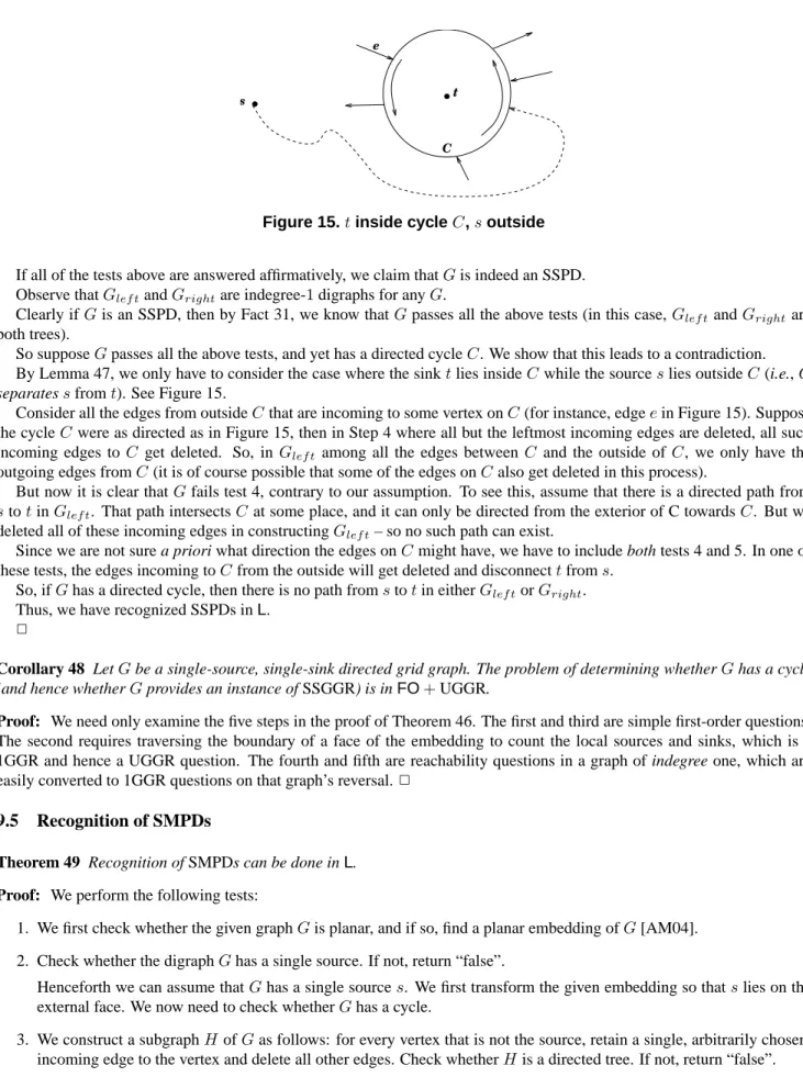
We study the complexity of restricted versions of s-t-connectivity, which is the standard complete problem forNL. In particular, we focus on different classes of planar graphs, of which grid graphs are an important special case. Our main results are:

• Reachability in graphs of genus one is logspace-equivalent to reachability in grid graphs (and in particular it is logspace-equivalent to both reachability and non-reachability in planar graphs).

• Many of the natural restrictions on grid-graph reachability (GGR) are equivalent underAC0reductions (for instance, undirected GGR, outdegree-one GGR, and indegree-one-outdegree-one GGR are all equivalent). These problems are all equivalent to the problem of determining whether a completed game position in HEX is a winning position, as well as to the problem of reachability in mazes studied by Blum and Kozen [BK78]. These problems provide natural examples of problems that are hard forNC1underAC0reductions but are not known to be hard forL; they thus give insight into the structure ofL.

• Reachability in layered planar graphs is logspace-equivalent to layered grid graph reachability (LGGR). We show that LGGR lies inUL(a subclass ofNL).

• Series-Parallel digraphs (on which reachability was shown to be decidable in logspace by Jakoby et al.) are a spe-cial case of single-source-single-sink planar directed acyclic graphs (DAGs); reachability for such graphs logspace reduces to single-source-single-sink acyclic grid graphs. We show that reachability on such grid graphsAC0reduces to undirected GGR.

• We build on this to show that reachability for single-source multiple-sink planar DAGs is solvable inL.

1

Introduction

Graph reachability problems play a central role in the study and understanding of subclasses ofP. Thes-t-connectivity problem for directed graphs (STCONN) is complete for nondeterministic logspace (NL); the restriction of this problem to undirected graphs, called USTCONN, was shown by Reingold to be complete for logspace (L) [Rei05]; thus this problem has the same complexity as the s-t-connectivity problem for graphs of outdegree 1 (and even for graphs of indegree and outdegree at most 1 [CM87, Imm87, Ete97]. It follows from [Bar89] that reachability in directed graphs of widthO(1)(or even width five, with outdegree 1) is complete forNC1.

∗_{Department of Computer Science, Rutgers, the State University of NJ. Supported in part by NSF Grant CCF-0514155. email:} [email protected].

†_{Computer Science Dept., University of Massachusetts Amherst. Supported in part by NSF Grant CCR-9988260. e-mail:[email protected].} ‡_{Computer and Information Science Department, University of Pennsylvania e-mail:[email protected].}

§_{Chennai Mathematical Institute, Chennai, India. e-mail:[email protected].}

1.1

Planar Graphs

Our focus in this paper is the restriction ofSTCONN to planar (directed) graphs: PLANAR.STCONN. This problem is hard forLunder uniform projections, as a consequence of [Ete97], and it lies inNL. Although there are a number of papers presenting efficient algorithms for connectivity in planar graphs (such as [Hus95, EIT+92, HKRS97]), little is known about the computational complexity of this problem. Prior to our work, the best upper bound known for PLANAR.STCONN was NL. Building on our work, Bourke, Tewari, and Vinodchandran recently showed that the GGR problem studied here is in Unambiguous Logspace (UL) [BTV07]. It follows that the class of problems≤log

m -reducible to PLANAR.STCONN can be

viewed as a complexity class lying betweenLandUL.

Grid graphs are an important restricted class of graphs for which the reachability problem has significant connections to

complexity classes. (The vertices in a grid graph are a subset ofIN×IN, and all edges are of the form(i, j)→(i+b, j)

or (i, j) → (i, j +b), where b ∈ {1,−1}.) In [BLMS98], Barrington et al. showed that the reachability problem in (directed or undirected) grid graphs of widthkcaptures the complexity of depthkAC0. In this paper we study grid graphs without any width restrictions. The construction of [BLMS98, Lemma 13] shows that GGR reduces to its complement via uniform projections. (The problemsSTCONNand USTCONNalso reduce to their complements via uniform projections, as a consequence of [Imm88, Sze88, Rei05, NTS95].) Reachability problems for grid graphs have proved easier to work with than the corresponding problems for general graphs. For instance, the reachability problem for undirected grid graphs (UGGR) was shown to lie inLin the 1970’s [BK78], although more than a quarter-century would pass before Reingold proved the corresponding theorem for general undirected graphs.

We show that PLANAR.STCONNis logspace-equivalent to GGR (and consequently it is logspace-reducible to its com-plement). (It had already been shown in [HRS93] that a special case of PLANAR.STCONN is logspace-reducible to its complement.) We do not know whether this reduction can be accomplished by uniform projections or even byNC1

reduc-tions; in contrast to the case forSTCONN,USTCONN, and GGR. We also show that thes-t-connectivity problem for graphs of genus one is logspace reducible to PLANAR.STCONN; the generalization for graphs of higher genus remains open.

1.2

Restrictions of Grid Graphs

We consider several natural restrictions of GGR in this paper. We have already mentioned UGGR (undirected grid graph reachability). Buss has studied UGGR in connection with tautologies arising from the game of HEX [Bus06] (namely, the tautology that every completed game board of HEX has a winner); he credits Barrington with the observation that UGGR is equivalent to the problem of determining whether a given completed HEX board position is a win for one player. Reachability in grid graphs of outdegree one (1GGR) is another restriction on GGR that is clearly solvable in logspace.

One of our theorems is that UGGR and 1GGR are equivalent underAC0reductions (and even under first-order projections). We show that these problems are hard forNC1, and thus this gives a cluster of natural problems that are candidates for having complexity intermediate betweenNC1andL, since even the general GGR problem is not known to be hard forLunderAC0 reductions.

A graph is said to be layered if the vertex set is partitioned into “layers”, where all edges from vertices in layerihave destinations in layeri+ 1. Just as general GGR is logspace-equivalent to reachability in planar digraphs, we observe that reachability in layered planar digraphs is logspace equivalent to the “layered” grid graph reachability problem (LGGR). In an instance of LGGR, all edges are directed either “east” or “south”. Thus without loss of generality, the start node is in the top left corner. If such a grid graph is rotated 45 degrees counterclockwise, one obtains a graph whose “columns” correspond to the diagonals of the original graph, wheresis the only node in the first “column”, and all edges in one column are directed “northeast” or “southeast” to their neighbors in the following column. This is consistent with the usual usage of the word “layered” in graph theory.

We show that LGGR lies in a subclass ofNLknown asUL. That is, LGGR is accepted by a nondeterministic logspace machine that never has more than one accepting computation path on a given input. Note that the the improvement fromNL toULis, at best, a very slight improvement; it is known [RA00] that the non-uniform versions ofULandNLare the same, and it is entirely plausible that the classes themselves are the same. In particular, it is shown in [ARZ99] thatNL=ULif there is any problem inDSPACE(n)that requires circuits of exponential size. We actually show that LGGR lies inUL∩coUL, since (in contrast to nearly all of the other reachability problems we consider) it remains open whether LGGR reduces to its complement. (Note also that it remains open whetherUL =coUL.) The work of Bourke et al. [BTV07] showing that PLANAR.STCONN∈ULbuilds on this theorem of ours. Subsequently,ULhas been shown to contain other graph-theoretic problems of interest [TW08]. Some other examples of reachability problems inULwere presented earlier by Lange [Lan97];

these problems are obviously inUL(in the sense that the positive instances consist of certain graphs that contain only one path from stot), and the main contribution of [Lan97] is to present a completeness result for a natural subclass of UL. In contrast, positive instances of LGGR can have many paths fromstot. We know of no reductions (in either direction) between LGGR and the problems considered in [Lan97].

1.3

Reachability Problems in Logspace

Jakoby, Liskiewicz, and Reischuk showed that reachability in series-parallel digraphs is solvable in logspace [JLR06], thus solving the reachability question for an important subclass of planar directed graphs. (They also show the much stronger result that counting the number of paths betweensandtcan be carried out in logspace for series-parallel graphs.) Series-parallel digraphs are a special case of planar directed acyclic graphs having a single source and single sink. Motivated by a desire to solve the reachability problem for a larger class of planar DAGs, we introduce the following three classes of DAGs:

• Single-Source Single-Sink Planar DAGs (SSPDs): the class of DAGs having one vertex of indegree zero and one vertex

of outdegree zero. Reachability in SSPDs generalizes the problem of reachability in series-parallel digraphs studied in [JLR06].

• Single-Source Multiple-Sink Planar DAGs (SMPDs): the class of DAGs having one vertex of indegree zero.

Reach-ability in such graphs is clearly equivalent to reachReach-ability in Multiple-Source Single Sink DAGs (MSPDs) by simply reversing all of the edges.

• Multiple-Source Multiple-Sink Planar DAGs (MMPD). This is simply the class of all planar DAGs.

We show that the SMPD reachability problem (and hence also that for MSPD) lies in logspace. In addition, reachability in SSPDs, restricted to grid graphs, is reducible to UGGR. Our algorithmic approach for SMPD extends to certain classes of graphs that are not acyclic. This is discussed in more detail in Section 9.

The rest of the paper is organized as follows. After a few preliminaries (Section 2), we begin by presenting results related to PLANAR.STCONN. In Section 3 we show that PLANAR.STCONNreduces to a special case wheresandtlie on the external face. This is useful in presenting our reduction from PLANAR.STCONNto GGR in Section 4. In Section 5 we prove a closure property of the class of sets logspace reducible to PLANAR.STCONN, and then in Section 6 we show that planar reachability is equivalent to reachability in genus one graphs. Next, in Section 7 we introduce the various restricted grid graph problems that we will be considering, and present reductions showing how these problems relate to each other. In Section 7.3 we present a generic reduction showing that, for many of the problems we consider, it is no loss of generality to assume that

sandtappear on the external boundary of the graph. (In some sense this is reminiscent of the results of Section 3). Our hardness results are presented in Section 8. Our logspace algorithms for SSPD and SMPD are presented in Section 9. We conclude with open questions in Section 10.

2

Classes and Reductions

We assume familiarity with the following important subclasses of nondeterministic logspace (NL):L,NC1,TC0, andAC0. When defining notions of reducibility and completeness in order to investigate the structure of such small complexity classes, some form ofAC0reducibility is usually employed. We will frequently make use of the terminology and notation employed by Immerman [Imm98], which exploits the close connections betweenAC0and first-order logic. In particular,AC0-Turing reducibility (≤AC0

T ) to a setAcan be defined equivalently in terms ofAC

0_{circuits augmented with “oracle gates” forA, or}

in terms of first-order formulae withAas a built-in predicate symbol applied to a structure defined in first-order. For details refer to [Imm98]. For this reason, we sometimes refer to≤AC0

T reductions asFOreductions. The class of problems≤ AC0 T

reducible toAis sometimes denoted asFO+A.

Immerman also gives good motivation for studying a restricted form of ≤AC0

m reductions called first-order projections

(≤FO

proj). These can be visualized as many-one reductions computed by first-order uniform circuits having no gates (other

than NOTgates); thus each bit of the output is either a constant or is a copy (or a negated copy) of one bit of the input. For example, the class depth-kAC0is closed under these reductions.

G’

t s

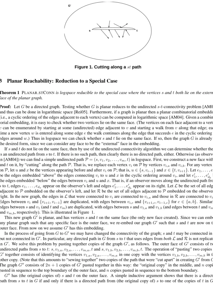
Figure 1. Cutting along astpath

3

Planar Reachability: Reduction to a Special Case

Theorem 1 PLANAR.STCONNis logspace reducible to the special case where the verticessandtboth lie on the external face of the planar graph.

Proof: LetGbe a directed graph. Testing whetherGis planar reduces to the undirecteds-t-connectivity problem [AM04] and thus can be done in logarithmic space [Rei05]. Furthermore, if a graph is planar then a planar combinatorial embedding (i.e., a cyclic ordering of the edges adjacent to each vertex) can be computed in logarithmic space [AM04]. Given a combina-torial embedding, it is easy to check whether two vertices lie on the same face. (The vertices on each face adjacent to a vertex

v can be enumerated by starting at some (undirected) edge adjacent tov and starting a walk fromv along that edge; each time a new vertexwis entered along some edgeethe walk continues along the edge that succeedsein the cyclic ordering of edges aroundw.) Thus in logspace we can check whethersandtlie on the same face. If so, then the graphGis already in the desired form, since we can consider any face to be the “external” face in the embedding.

Ifsandtdo not lie on the same face, then by use of the undirected connectivity algorithm we can determine whether there is an undirected path fromstot. If there is no such path, then clearly there is no directed path, either. Otherwise (as observed in [AM04]) we can find a simple undirected pathP= (s, v1, v2, . . . , vm, t)in logspace. First, we construct a new face withs

andton it, by “cutting” along the pathP. That is, we replace each vertexvionP by verticesvi,aandvi,b. For any vertexvi

onP, letuandxbe the vertices appearing before and aftervionP; that is,u∈ {s, vi−1}andx∈ {t, vi+1}. Lete1, . . . , eda

be the edges embedded “above” the edges connectingvi touandxin the cyclic ordering aroundvi, and lete01, . . . , e0db be

the edges embedded “below” the edges betweenvianduandx. That is, if an observer moves along the undirected path from stot, edgese1, . . . , edaappear on the observer’s left and edgese

0

1, . . . , e0db appear on its right. LetLbe the set of all edges

adjacent toP embedded on the observer’s left, and letRbe the set of all edges adjacent toP embedded on the observer’s right. In the new graph, the edges inLthat were connected toviare connected tovi,aand those inRare connected tovi,b.

Edges betweenviand{vi+1, vi−1} are duplicated, with edges betweenvi,c and{vi+1,c, vi−1,c}forc ∈ {a, b}. Similarly,

edges betweensandv1(andtandvm) are duplicated, with edges betweensandv1,aandv1,b(and edges betweentandvm,a

andvm,b, respectively). This is illustrated in Figure 1.

This new graphG0 _{is planar, and has verticessandton the same face (the only new face created). Since we can embed} any planar graph such that any specific face is the outer face, we re-embed our graphG0 such thatsandtare now on the outer face. From now on we assumeG0has this embedding.

In the process of going fromGtoG0we may have changed the connectivity of the graph;sandtmay be connected inG

but not connected inG0. In particular, any directed path inGfromstotthat uses edges from bothLandRis not replicated inG0. We solve this problem by pasting together copies of the graphG0, as follows. The outer face ofG0 consists of two undirected paths fromstot:s, v1,a, v2,a, . . . , vm,a, tands, v1,b, v2,b, . . . , vm,b, t. The operation of “pasting” two copies of G0 together consists of identifying the verticesv1,a, v2,a, . . . , vm,ain one copy with the verticesv1,b, v2,b, . . . , vm,b in the

other copy. (Note that this amounts to “sewing together” two copies of the path that were “cut apart” in creatingG0fromG.) The graphG00consists of2n+ 1copies ofG0 pasted together in this way: the “original copy” in the middle, andncopies pasted in sequence to the top boundary of the outer face, andncopies pasted in sequence to the bottom boundary.

G00 has (the original copies of)sandton the outer face. A simple inductive argument shows that there is a directed path fromstotinGif and only if there is a directed path from (the original copy of)sto one of the copies oftinG00.

s t G

P

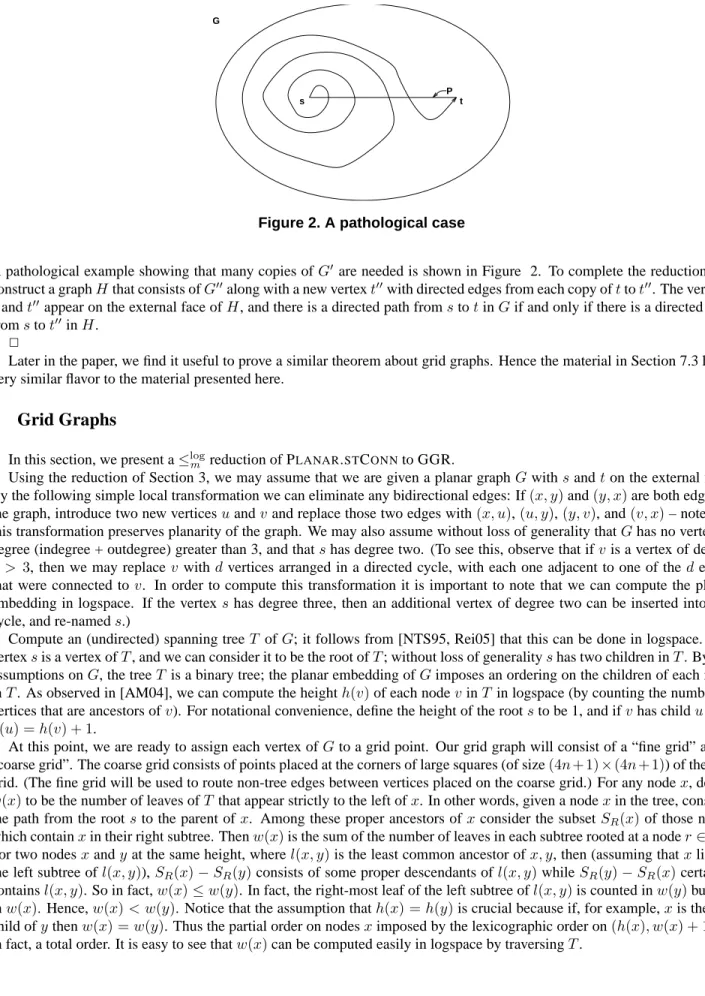
Figure 2. A pathological case

A pathological example showing that many copies ofG0are needed is shown in Figure 2. To complete the reduction, we construct a graphHthat consists ofG00along with a new vertext00with directed edges from each copy ofttot00. The vertices

sandt00appear on the external face ofH, and there is a directed path fromstotinGif and only if there is a directed path fromstot00_inH.

2

Later in the paper, we find it useful to prove a similar theorem about grid graphs. Hence the material in Section 7.3 has a very similar flavor to the material presented here.

4

Grid Graphs

In this section, we present a≤log

m reduction of PLANAR.STCONNto GGR.

Using the reduction of Section 3, we may assume that we are given a planar graphGwithsandton the external face. By the following simple local transformation we can eliminate any bidirectional edges: If(x, y)and(y, x)are both edges in the graph, introduce two new verticesuandvand replace those two edges with(x, u),(u, y),(y, v), and(v, x)– note that this transformation preserves planarity of the graph. We may also assume without loss of generality thatGhas no vertex of degree (indegree + outdegree) greater than 3, and thatshas degree two. (To see this, observe that ifvis a vertex of degree

d > 3, then we may replacev withdvertices arranged in a directed cycle, with each one adjacent to one of thededges that were connected tov. In order to compute this transformation it is important to note that we can compute the planar embedding in logspace. If the vertexshas degree three, then an additional vertex of degree two can be inserted into this cycle, and re-nameds.)

Compute an (undirected) spanning treeT ofG; it follows from [NTS95, Rei05] that this can be done in logspace. The vertexsis a vertex ofT, and we can consider it to be the root ofT; without loss of generalityshas two children inT. By our assumptions onG, the treeT is a binary tree; the planar embedding ofGimposes an ordering on the children of each node inT. As observed in [AM04], we can compute the heighth(v)of each nodevinTin logspace (by counting the number of vertices that are ancestors ofv). For notational convenience, define the height of the rootsto be 1, and ifvhas childuthen

h(u) =h(v) + 1.

At this point, we are ready to assign each vertex ofGto a grid point. Our grid graph will consist of a “fine grid” and a “coarse grid”. The coarse grid consists of points placed at the corners of large squares (of size(4n+ 1)×(4n+ 1)) of the fine grid. (The fine grid will be used to route non-tree edges between vertices placed on the coarse grid.) For any nodex, define

w(x)to be the number of leaves ofT that appear strictly to the left ofx. In other words, given a nodexin the tree, consider the path from the rootsto the parent ofx. Among these proper ancestors ofxconsider the subsetSR(x)of those nodes

which containxin their right subtree. Thenw(x)is the sum of the number of leaves in each subtree rooted at a noder∈SR.

For two nodesxandyat the same height, wherel(x, y)is the least common ancestor ofx, y, then (assuming thatxlies in the left subtree ofl(x, y)),SR(x)−SR(y)consists of some proper descendants ofl(x, y)whileSR(y)−SR(x)certainly

containsl(x, y). So in fact,w(x)≤w(y). In fact, the right-most leaf of the left subtree ofl(x, y)is counted inw(y)but not inw(x). Hence,w(x)< w(y). Notice that the assumption thath(x) =h(y)is crucial because if, for example,xis the left child ofythenw(x) =w(y). Thus the partial order on nodesximposed by the lexicographic order on(h(x), w(x) + 1)is, in fact, a total order. It is easy to see thatw(x)can be computed easily in logspace by traversingT.

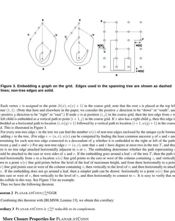
Figure 3. Embedding a graph on the grid. Edges used in the spanning tree are shown as dashed lines; non-tree edges are solid.

Each vertexxis assigned to the point(h(x), w(x) + 1)in the coarse grid; note that the rootsis placed at the top left corner(1,1). (Note that here and elsewhere in the paper, we consider the positivexdirection to be “down” or “south”, and the positiveydirection to be “right” or “east”.) If nodexis at position(i, j)in the coarse grid, then the tree edge fromxto its left child is embedded as a vertical path to point(i+ 1, j)in the coarse grid. Ifxalso has a right childy, then this edge is embedded as a horizontal path to location(i, w(y) + 1)followed by a vertical path to location(i+ 1, w(y) + 1)in the coarse grid. This is illustrated in Figure 3.

For every non-tree edgeein the tree we can find the numberw(e)of non-tree edges enclosed by the unique cycle formed by addingeto the tree. (For edgee= (u, v),w(e)can be computed by finding the least common ancestoryofuandvand determining for each non-tree edge connected to a descendant ofywhether it is embedded to the right or left of the paths betweenyanduandv.) For any non-tree edgee= (u, v), note thatuandvhave degree at most two in the treeT, and thus there is no tree edge attached horizontally adjacent touorv. The embedding determines whether the path representinge

should be attached to the east or west sides ofuandv. If the embedding goes around a leafzof the treeT, then the path is routed horizontally fromuto a locationw(e)fine grid points to the east or west of the column containingz, and vertically down to a pointw(e)fine grid points below the level of the leaf of maximum height, and from there horizontally to a point

w(e)fine grid points east or west of the column containingv, then vertically to the level ofv, and then horizontally to attach tov. If the embedding does not go around a leaf, then a simpler path can be drawn: horizontally to a pointw(e)fine grid points east or west ofv, then vertically to the level ofv, and then horizontally to connect tov. It is easy to verify that no paths collide in this way. See Figure 3 for an example.

Thus we have the following theorem.

Theorem 2 PLANAR.STCONN≤log_m GGR

Combining this theorem with [BLMS98, Lemma 13], we obtain this corollary:

Corollary 3 PLANAR.STCONNis≤log

m reducible to its complement.

5

More Closure Properties for P

.

C

We have identified an important problem PLANAR.STCONNthat may or may not be in the classL. If it is not, it is by definition complete under logspace reductions for a complexity class. Is this class robust under different types of logspace reductions? We are able to give a partial affirmative answer. Let us first remind the reader about some relevant definitions.

Different types of logspace reductions were introduced and studied by Ladner and Lynch [LL76], who showed that logspace Turing and truth-table reducibilities coincide (A≤log_T BiffA≤logtt B). They also introduced a more restrictive version

of logspace-computable truth-table reducibility, known as logspace Boolean formula reducibility≤log_bf−tt.A≤log_bf−ttBif there is a logspace computable functionfsuch thatf(x) = (q1, q2, . . . , qr, φ)where eachqiis a query andφis a Boolean formula

withrvariablesy1, . . . , yr, such thatx∈Aif and only ifφevaluates to 1 when the variablesyiare assigned the truth value

of the statement “qi∈B”. Additional results about this type of reducibility can be found in [BST93, BH91].

Corollary 4 A≤log

m PLANAR.STCONNif and only ifA≤ log

bf−ttPLANAR.STCONN.

Proof: One direction is trivial; thus assume thatA≤log_bf−ttPLANAR.STCONN. For a given inputx, letf(x) = (q1, q2, . . . , qr, φ)

be the result of applying the reduction tox. Without loss of generality, the formulaφhas negation operations only at the leaves (since it is easy in logspace to apply DeMorgan’s laws to rewrite a formula). Using closure under complementation, we can even assume that there are no negation operations at all in the formula. By the results of Section 3, we can assume that each graphqiis a planar graph withsandton the external face. Given two such graphsG1, G2, note that bothG1and G2are in PLANAR.STCONNif and only if the graph with the terminal vertex ofG1connected to the start vertex ofG2is in PLANAR.STCONN, and thus it is easy to simulate an AND gate. Similarly, an ORgate can be simulated by building a new graph with start vertexsconnected to the start vertices of bothG1andG2, and with edges from the terminal vertices ofG1

andG2to a new vertext. These constructions maintain planarity, and they also maintain the property thatsandtare on the external face. Simulating each gate in turn involves only a constant number of additional vertices and edges, and it is easy to see that this gives rise to a≤log

m reduction.2

A natural open question is whether the preceding corollary also holds, when≤log_bf−tt is replaced by≤log_T .

6

Higher Genus

In this section we prove that thes-t-connectivity problem for graphs of genus one reduces to the planar case. Throughout this section, we will assume that we are given an embeddingΠof a graphGonto a surface of genus one. (Unlike the planar case, it does not appear to be known if testing whether a graph has genusg > 0can be accomplished in logspace, even for

g= 1[MV00].) Given such an embedding, using [AM04], we can check in logspace whether the minimal genus of the graph is one.

We introduce here some terminology and definitions relating to graphs on surfaces. It will be sufficient to give informal definitions of various notions; the interested reader can refer to [MT01] for more rigorous definitions.

A closed orientable surface is one that can be obtained by adding handles to a sphere in3-space. The genus of the resulting surface is equal to the number of handles added; see also the text [GT87]. Given a graphG, the genus of the graph is the genus of the (closed orientable) surface of least genus on which the graph can be embedded.

Given a graphGembedded on a closed orientable surface, and a cycle of the graph embedded on the surface, there are two (possibly intersecting) subgraphs, called the two sides of the cycle with respect to the embedding. Informally, a side of a cycle is the set of vertices of the graph that are path-connected (via a path in the graph, each edge of the graph being considered regardless of direction) to some vertex on the cycle, such that this path does not cross the cycle itself. (In the considerations below, we are concerned only with genus one graphs for which this notion of path-connectivity suffices.) A cycle thereby has two sides, which are called the left and the right sides. If the left and right sides of a cycle have nonempty intersection, then we call the cycle a surface-nonseparating cycle. Note that a graph embedded on a sphere (i.e., a planar graph) does not have any surface-nonseparating cycles. Also, it is easy to see that a facial cycle (one that forms the boundary of a face in the embedding of the graph on the surface) cannot be surface-nonseparating. Given a cycleCin an embedded graph, it is easy to check in logspace whetherCis surface-nonseparating: merely check whether there is a vertexv ∈ G, such thatvis path-connected to both sides ofC(on the embedding).

Lemma 5 LetGbe a graph of genusg >0, and letT be a spanning tree ofG. Then there is an edgee∈E(G)such that T∪ {e}contains a surface-nonseparating cycle.

Proof: The proof follows ideas from [Tho90] which introduces the “3-path condition”:

Definition 6 LetKbe a family of cycles ofGas follows. We say thatKsatisfies the3-path condition if it has the following property. Ifx, yare vertices ofGandP1, P2, P3are internally disjoint paths joiningxandy, and if two of the three cycles Ci,j=Pi∪Pj(1≤i < j≤3) are not inK, then also the third cycle is not inK.

We quote the following from [MT01].

Proposition 7 (Proposition4.3.1of [MT01]) The family ofΠ-surface-nonseparating cycles satisfies the3-path condition.

Suppose, that∀e,(T ∪ {e})does not have a surface-nonseparating cycle. We will prove that no cycleC in the graph

Gcan be surface-nonseparating, by induction on the numberkof non-tree edges inC. This contradicts the fact that every non-planar graph has a surface-nonseparating cycle ([MT01, Lemma 4.2.4 and the following discussion]) and thus suffices to prove the claim.

The basis (k= 1) follows from the above supposition.

For the inductive step fromk−1tok, let a cycleCbe given withkedges not inT.

Take any non-tree edgee= (x, y)onC. Consider the tree pathPbetweenxandy. IfP never leaves the cycleC, then

Cis a fundamental cycle and we are done by the assumption fork= 1. Otherwise, we can consider a maximal segmentSof

P not inC. LetSlie between verticesuandvofC. Now, we have three paths betweenuandv: the two paths betweenu

andvonC(call theseC1,C2), and pathS. Note that bothS∪C1andS∪C2have fewer thanknon-tree edges. Hence they are not surface-nonseparating cycles by the induction assumption. So, by the3-path condition, neither isC=C1∪C2.

This completes the induction, and the proof.2

At this point we are able to describe how to reduce thes-t-connectivity problem for graphs of genus one to the planar case.

Given a graphGof genus one and an embeddingΠofGonto the torus, construct an (undirected) spanning treeT ofG. For each edgeeofGthat is not inT, determine whether the unique cycleCeinT∪ {e}is surface-nonseparating, as follows.

LetCe={v1, v2,· · ·, vr}. LetGebe the graph obtained fromGby cutting along the cycleCe(as described in [MT01,

p. 105]). (For the purposes of visualization, it is useful to imagine cycles as embedded on an inner tube. Cutting along a surface-separating cycle amounts to cutting a hole in the inner tube (resulting in two pieces). In contrast, ifCeis

surface-nonseparating, then it is embedded either like a ribbon tied around the tube, or like a whitewall painted on the inner tube. In the former case, cutting alongCe turns the inner tube into a bent cylinder with a copy ofCe on each end; in the latter

case cutting alongCeresults in a flat ring with one copy ofCearound the inside and one around the outside. In this latter

case, the graph is again topologically equivalent to a cylinder with a copy ofCeon each side.) More formally, the graphGe

has two copies of each of the vertices{v1, v2,· · ·, vr}, which we denote by{v1,1, v2,1,· · ·, vr,1}, and{v1,2, v2,2,· · ·, vr,2}.

For every edge(u, vj)(or(vj, u)) on the right side ofCe(according toΠ),Gehas the edge(u, vj,1)((vj,1, u), respectively),

and for every edge(u, vj)((vj, u),respectively) on the left side ofCewe have the edge(u, vj,2)(or(vj,2, u)) inGe. The

graphGealso has two copies of the cycleCe, which we denote byCe,1andCe,2. That is, we have edges betweenvj,band vj+1,b for eachb ∈ {1,2} and each1 ≤ j ≤ r, directed as inCe. An important property of cutting along the cycle Ce

is that ifCewas surface-nonseparating, then the resulting graphGeis planar, and the the cyclesCe,1andCe,2are facial

cycles ([MT01, p. 106,Lemma 4.2.4]). (Otherwise,Gewill not be planar.) Thus in logspace we can determine whetherCeis

surface-nonseparating.

By Lemma 5, we are guaranteed to find a surface-nonseparating cycle by testing each edgeethat is not inT. The graph

Gedoes not have the same connectivity properties asG;sandtmight have been connected inGbut not inGe. In particular,

any directed path inGfromstotthat uses edges from both the right and left sides ofCeis not replicated inGe. As in Section

3, we solve this problem by pasting together copies of the graphGe, as follows. The operation of “pasting” two copies ofGe

together consists of identifying the verticesv1,1, v2,1, . . . , vr,1in one copy with the verticesv1,2, v2,2, . . . , vm,2in the other

copy. (Note that this amounts to “sewing together” two copies of the path that were “cut apart” in creatingGefromG.)

Now construct the graphG0 consisting of2n+ 1copies ofGepasted together in this way: the “original copy” in the

middle, andncopies along each side, forming one long cylinder. Since this cylinder has genus zero, it is easy to see thatG0

is planar.

As in Section 3, a simple inductive argument shows that there is a directed path fromstotinGif and only if there is a directed path from (the original copy of)sto one of the copies oftinG0. Thus we have presented a logspace-computable disjunctive truth-table reduction to the planar directeds-t-connectivity problem. We obtain a many-one reduction by appeal to Corollary 4. Thus we have proved the following theorem.

Theorem 8 Thes-t-connectivity problem for graphs of genus one is≤log

m reducible to the planar directeds-t-connectivity problem.

GGR

11LGGR

1LGGR

11GGR-B

11GGR

1GGR-B

LGGR

GGR-B

1-GGR

Figure 4. NineGGRproblems.

7

Versions of the GGR Problem

Up until this point in the paper, we have not needed to be very careful about the way that grid graphs are encoded. However, many of the results in this and later sections discuss completeness and equivalence under first-order projections – and in order for us to easily establish reducibility via projections in some instances, we must impose some restrictions upon the encoding. It will be clear to the reader that the encodings that we use are equivalent to other, more natural, encodings, under≤AC0

m reductions. As a consequence of Propositions 15 and 16, it follows that the more natural encodings are, in fact,

reducible to these more restricted versions under projections, and hence they are equivalent under first-order projections. An instance of the general GGR problem consists of a graphGon ann-by-mgrid, along with two distinguished vertices

sandt. However, for the rest of this paper, we will restrict attention to graphs on a grid of size3n-by-3nwithsin position

(n, n)andtin position(2n,2n). It is easy to see how to transform an arbitrary grid graph instance into an instance withs

andtin these designated positions via an≤AC0

m reduction, by “stretching” (and possibly reflecting) the original grid.

We continue by defining and exploring a number of special cases of the GGR problem, based on a variety of restrictions on the grid graphs and on the verticessandt.

7.1

Nine Problems

We first consider two restrictions on the global structure of a GGR problem, and two local restrictions:

• The problem GGR-B is the set of directed grid graphsGwheresandtare vertices on the boundary ofG, and there is a path fromstotinG. (Equivalently,Gis ann-by-ngrid, withsin position(1,1)andtin position(n, n).)

• The problem LGGR is the set of layered directed grid graphsG, having only east and south edges, where there is a path fromstot. (Again, we use the convention thatsis in position(1,1)andtis in position(n, n).)

• The problem 1GGR is the set of directed grid graphsGof outdegree at most 1 where there is a path fromstot. (Since a cycle of length two can not contribute to a path fromstot, and since the existence of such cycles makes certain of our reductions more complicated, and since such cycles are easy to eliminate via a syntactic test, we assume that there is no cycle of length 2 in an instance of 1GGR.)

• The problem 11GGR is the set of directed grid graphsGof indegree and outdegree at most 1 where there is a path fromstot.

It is obvious that 11GGR is a special case of 1GGRand LGGR is a special case of GGR-B. The local and global restrictions are orthogonal, so that the three global conditions (general, boundary, and layered) and three local conditions (general,

outdegree 1, both degrees 1) give us nine special cases of the GGR problem: GGR, 1GGR, 11GGR, GGR-B, 1GGR-B, 11GGR-B, LGGR, 1LGGR, and 11LGGR. Even the easiest of these problems, 11LGGR, is non-trivial, as we will show in Section 8 that it is hard for the classTC0.

There are other natural ways to define a layered graph. We could forbid only one of the four directions of edges rather than two. Or we could allow diagonal edges but force them to go only northeast, east, or southeast, making each north-south column a layer according to the standard definition. But it is an easy exercise to construct a first-order projection from a graph satisfying any one of these restrictions to one satisfying any of the others. (We prove a very similar result in Proposition 26.)

7.2

Undirected GGR

One of the most natural local restrictions on a graph is undirectedness. Long before Reingold [Rei05] showed that the undirected reachability problem is inL, Blum and Kozen [BK78] showed that the UGGR problem, testing reachability in undirected grid graphs, is inL. Here we show that UGGR is equivalent to four of the nine versions of GGR we have just defined:

Theorem 9 The problems UGGR, UGGR-B, 1GGR, 1GGR-B, 11GGR, and 11GGR-B are all equivalent under first-order

projections.

Proof: We will show that 1GGR≤FO

projUGGR≤FOprojUGGR-B≤FOproj11GGR-B≤FOproj1GGR,appealing to Section 7.3 for the

second reduction and observing that the last reduction is trivial.

Lemma 10 1GGR≤FO projUGGR

Proof: The well-known general reduction from outdegree one reachability to undirected reachability works without

modifi-cation for grid graphs. Given an outdegree one grid graphGand verticessandt, create an undirected graphHby modifying

Gto delete the edge (if any) out oftand change each directed arc to an undirected edge. Since the vertices with paths totin

Gform a directed tree, the corresponding vertices inHare simplyt’s connected component. Soshas a directed path totin

Gif and only if it has an undirected path totinH. The reduction is clearly a first-order projection.2

Lemma 11 UGGR-B≤FO

proj11GGR-B

Proof: We merely have to formalize the familiar “right-hand rule” for exploring mazes – if we place our right hand on the

wall and keep walking with our hand on the wall, we will return to our starting place having gone completely around the connected component of wall to our right. If both our starting place and our goal are on the boundary of the entire maze, they are on the boundary of their connected component.

More formally, given an undirected grid graph Gand vertices s andt on its boundary, we define a grid graph H of indegree and outdegree at most 1 as follows. The vertices ofH will be points(a/3, b/3)whereaandbare integers – when both coordinates are integers we identify this vertex of H with the corresponding vertex ofG. (Note that the positivex

direction is east, and the positiveydirection is south.) The directed edges ofHwill have the property that there is an edge of

G1/3unit to their right in their direction of travel, unless they are turning a corner:

• If there is an edge inGbetween(u, v)and(u+ 1, v), then there are directed arcs inH from(u+ 1/3, v−1/3)to

(u+ 2/3, v−1/3)and from(u+ 2/3, v+ 1/3)to(u+ 1/3, v+ 1/3).

• If there is an edge inGbetween(u, v)and(u, v+ 1), then there are directed arcs inH from(u−1/3, v+ 2/3)to

(u−1/3, v+ 1/3)and from(u+ 1/3, v+ 1/3)to(u+ 1/3, v+ 2/3).

• If(u, v)is a vertex ofGwith no edge inGto(u+ 1, v), thenH has edges from(u+ 1/3, v−1/3)to(u+ 1/3, v)

and from(u+ 1/3, v)to(u+ 1/3, v+ 1/3).

• If(u, v)is a vertex ofGwith no edge inGto(u−1, v), thenH has edges from(u−1/3, v+ 1/3)to(u−1/3, v)

and from(u−1/3, v)to(u−1/3, v−1/3).

• If(u, v)is a vertex ofGwith no edge inGto(u, v+ 1), thenH has edges from(u+ 1/3, v+ 1/3)to(u, v+ 1/3)

t’ s’

t s

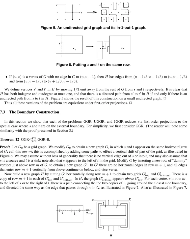
Figure 5. An undirected grid graph and its in-1-out-1 graph.

t s

t s

Figure 6. Puttingsandton the same row.

• If(u, v)is a vertex ofGwith no edge inGto(u, v−1), thenH has edges from(u−1/3, v−1/3)to(u, v−1/3)

and from(u, v−1/3)to(u+ 1/3, v−1/3).

We define verticess0andt0inH by moving1/3unit away from the rest ofGfromsandtrespectively. It is clear that

H has both indegree and outdegree at most one, and that there is a directed path froms0tot0inH if and only if there is an undirected path fromstotinH. Figure 5 shows the result of this construction on a small undirected graph.2

Thus all these versions of the problem are equivalent under first-order projections.2

7.3

The Boundary Construction

In this section we show that each of the problems GGR, UGGR, and 1GGR reduces via first-order projections to the special case wheresandtare on the external boundary. For simplicity, we first consider GGR. (The reader will note some similarity with the proof presented in Section 3.)

Theorem 12 GGR≤FO

projGGR-B.

Proof: LetG0be a grid graph. We modifyG0to obtain a new graphG, in whichsandtappear on the same horizontal row ofG; call this rowm; this is accomplished by adding some paths to effect a vertical shift of part of the grid, as illustrated in Figure 6. We may assume without loss of generality that there is no vertical edge out ofsor intot, and may also assume that

sis a source andtis a sink; note also thatsappears to the left oftin the grid. ModifyGby inserting a new row of “dummy” vertices just above rowmofG, to obtain a new graphG0. InG0there are no horizontal edges in rowm+ 1, and all edges that enter rowm+ 1vertically from above continue on below, and vice-versa.

Now build a new graphH by cuttingG0horizontally along rowm+ 1to obtain two gridsG0_topandG0_bottom. There is a copy of rowm+ 1in each ofG0_topandG0_bottom. InH, the graphG0_bottomappears aboveG0_top. For each vertexvin rowm1

to the left ofsor to the right oft, there is a path connecting the the two copies ofv, going around the closest side boundary, and directed the same way as the edge that passes throughvinG, as illustrated in Figure 7. Also as illustrated in Figure 7,

s t m

m+1

s t

H

s’ t’

H H H 0 s’ 0 -1 1 -1 1 t’ t’ t’ 0 t"

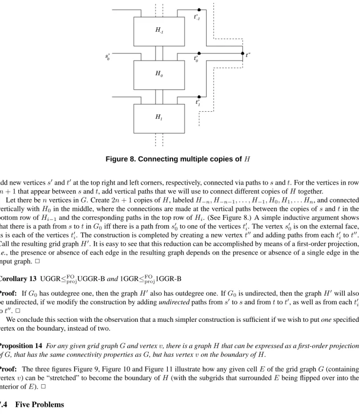
Figure 8. Connecting multiple copies ofH

add new verticess0andt0at the top right and left corners, respectively, connected via paths tosandt. For the vertices in row

m+ 1that appear betweensandt, add vertical paths that we will use to connect different copies ofH together.

Let there benvertices inG. Create2n+ 1copies ofH, labeledH−n, H−n−1, . . . , H−1, H0, H1, . . . Hn, and connected

vertically withH0in the middle, where the connections are made at the vertical paths between the copies ofsandtin the

bottom row ofHi−1and the corresponding paths in the top row ofHi. (See Figure 8.) A simple inductive argument shows

that there is a path fromstotinG0iff there is a path froms00 to one of the verticest0i. The vertexs00is on the external face,

as is each of the verticest0_i. The construction is completed by creating a new vertext00and adding paths from eacht0_itot00. Call the resulting grid graphH0. It is easy to see that this reduction can be accomplished by means of a first-order projection,

i.e., the presence or absence of each edge in the resulting graph depends on the presence or absence of a single edge in the

input graph.2

Corollary 13 UGGR≤FO

projUGGR-B and 1GGR≤FOproj1GGR-B

Proof: IfG0has outdegree one, then the graphH0also has outdegree one. IfG0is undirected, then the graphH0will also be undirected, if we modify the construction by adding undirected paths froms0tosand fromttot0, as well as from eacht0_i

tot00.2

We conclude this section with the observation that a much simpler construction is sufficient if we wish to put one specified vertex on the boundary, instead of two.

Proposition 14 For any given grid graphGand vertexv, there is a graphHthat can be expressed as a first-order projection ofG, that has the same connectivity properties asG, but has vertexvon the boundary ofH.

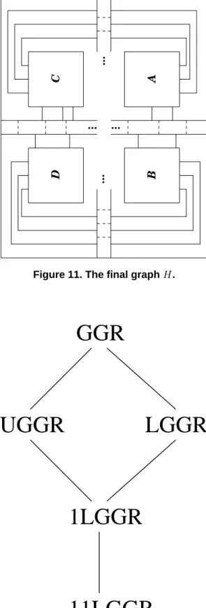
Proof: The three figures Figure 9, Figure 10 and Figure 11 illustrate how any given cellEof the grid graphG(containing vertexv) can be “stretched” to become the boundary ofH (with the subgrids that surroundedEbeing flipped over into the interior ofE).2

7.4

Five Problems

The results of the preceding section and of Section 7.3 reduce our nine problems to five. If we close each under first-order reductions, we get a hierarchy of complexity classes withinNLand (as we shall see in Section 8) aboveTC0. Since each problem has a number of interesting alternate formulations, we spend some time looking at each in turn:

00 00

11 11

A

B

D

C

....

....

....

....

....

....

....

....

Figure 9. Grid graphGwith cellEin the center.

C

D

A

B

... ... ... ... A B C D

Figure 11. The final graphH.

UGGR

LGGR

1LGGR

11LGGR

GGR

7.4.1 GGR

We have already presented most of our theorems regarding the general GGR problem (namely, that GGR is equivalent to reachability in planar graphs under logspace reductions). We showed in Section 7.3 that GGR and GGR-B are equivalent under first-order reductions. We have also already mentioned that GGR∈UL[BTV07].

It is worth spending a paragraph discussing whether GGR is complete forNL. Since many would conjecture thatNL=

UL, the fact that GGR ∈ ULis not strong evidence that GGR is not complete for NL, although it certainly qualifies as circumstantial evidence. Additional circumstantial evidence for its not being complete for NLcomes from the following observations:

• GGR is not even known to be hard forL under first-order reductions; for all other known examples of complete problems forNLhardness forLis essentially trivial.

• The proof of the Immerman-Szelepcs´enyi theorem [Imm88, Sze88] showing thatNLis closed under complement bears little relation to the simple argument showing that GGR reduces to its complement. (Namely there is no path fromsto

tin a grid graphGiff there is a path, from some boundary vertex on one path fromstotto a boundary vertex on the other path, in the complement-dual grid graph. For details see [BLMS98].)

It has been noticed by Jakoby and Tantau [JT06] that GGR is equivalent under first-order projections to a restriction of GGR that they call “tournament grid graphs”. Such graphs are obtained from a complete undirectedn×ngrid by assigning a direction to each edge.

We close this section with an observation about closure under first-order reductions: ¿

Proposition 15 A language is in the classFO+GGR iff it projection-reduces to GGR. The proof is identical to the proof of Proposition 16 in the next section.

7.4.2 UGGR

We found above that UGGR, undirected grid graph reachability, has a number of equivalent formulations including its boundary version UGGR-B. To these we may add the problem of determining the winner in a completed game of HEX [Bus06], because a hexagonal grid can easily be mapped by a projection reduction to the Euclidean grids we have defined here. Like GGR-B, UGGR-B projection-reduces directly to its complement by taking a complement-dual graph. This gives it another robustness property:

Proposition 16 A language is in the classFO+UGGR iff it projection-reduces to UGGR.

Proof: We show that the set of languages that projection-reduce to UGGR-B, and hence (by Section 7.3) to UGGR, is closed

under≤AC0

T reductions. We give an inductive argument on the depth of the circuits computing the≤AC 0

T reduction (where

without loss of generality the circuits for different lengths have the same structure, and all gates on the same level are of the same type). The inductive hypothesis is that the value of each wirewleading into a top-level gate can be represented as the answer to the question of whether or not a graphGwis in UGGR-B whereGwis a projection of the input graphG. This is

clearly true if the only gates are NOTgates, which establishes the basis for the induction. If the top-level gate is an ANDgate, then it suffices to connect the graphsGwin series. Similarly, if the top-level gate is an ORgate, then it suffices to connect

the graphsGwin parallel. If the top level gate is a NOTgate, then as we observed above, the complement-dual graph lets

us represent the negation of a UGGR-B problem as the ORof polynomially many UGGR-B problems (and thus again we can connect these graphs in parallel.) If the top level gate is an oracle gateg, then we can replace each wirew(representing an edge (x, y)in the encoding of the grid graphH presented as input tog) by a small sub-grid encoding the graphGw,

identifying the source vertex asxand the sink vertex asy. The details are straightforward to fill in; by simple padding we may assume that all of the graphsGware the same size.2

In its incarnation as 11GGR, UGGR can be seen to have the following counting property:

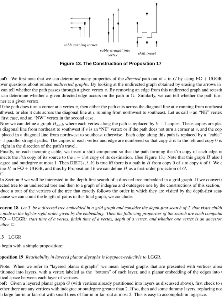
Proposition 17 If Gis a directed grid graph of indegree and outdegree each at most one, then the following predicate projection-reduces to UGGR: DIST(s, t, k)↔the path out ofsreachestin exactlyksteps.

cable turning corner

cable straight into

shift insert vertex

Figure 13. The Construction of Proposition 17

Proof: We first note that we can determine many properties of the directed path out ofsinGby usingFO+UGGR to answer questions about related undirected graphs. By looking at the undirected graph obtained by erasing the arrows inG, we can tell whether the path passes through a given vertexv. By removing an edge from this undirected graph and retesting, we can determine whether a given directed edge occurs on the path inG. Similarly, we can tell whether the path turns a corner at a given vertex.

If the path does turn a corner at a vertexv, then either the path cuts across the diagonal line atvrunning from northeast to southwest, or else it cuts across the diagonal line atvrunning from northwest to southeast. Let us callvan “NE” vertex in the first case, and an “NW” vertex in the second case.

Now we can define a graphHs,t,kwhere each vertex along the path is replaced byk+ 1copies. These copies are placed

in a diagonal line from northeast to southwest ifvis an “NE” vertex or if the path does not turn a corner atv, and the copies are placed in a diagonal line from northwest to southeast otherwise. Each edge along this path is replaced by a “cable” of

k+ 1parallel straight paths. The copies of each vertex and edge are numbered so that copykis to the left and copy0is to the right in the direction of the path’s travel.

Finally, on each incoming cable, we insert a shift component so that the path forming thei’th copy of each edge now connects thei’th copy of its source to thei+ 1’st copy of its destination. (See Figure 13.) Note that this graphHalso has indegree and outdegree at most 1. Then DIST(s, t, k)is true iff there is a path inHfrom copy0ofsto copykoft. We can defineH inFO+UGGR, and thus by Proposition 16 we can defineHas a first-order projection ofG.

2

In Section 9 we will be interested in the depth-first search of a directed tree embedded in a grid graph. If we convert the directed tree to an undirected tree and then to a graph of indegree and outdegree one by the constructions of this section, we produce a tour of the vertices of the tree that exactly follows the order in which they are visited by the depth-first search. Because we can count the length of paths in this final graph, we conclude:

Theorem 18 LetT be a directed tree embedded in a grid graph and consider the depth-first search ofT that visits children of a node in the left-to-right order given by the embedding. Then the following properties of the search are each computable inFO+UGGR: start time of a vertex, finish time of a vertex, depth of a vertex, and whether one vertex is an ancestor of

another.2

7.4.3 LGGR

We begin with a simple proposition:;

Proposition 19 Reachability in layered planar digraphs is logspace-reducible to LGGR.

Note: When we refer to “layered planar digraphs” we mean layered graphs that are presented with vertices already partitioned into layers, with a vertex labeled as the “bottom” of each layer, and a planar embedding of the edges into the vertical space between each layer of vertices.

Proof: Given a layered planar graphG(with vertices already partitioned into layers as discussed above), first check to see whether there are any vertices with indegree or outdegree greater than 2. If so, then add some dummy layers, replacing nodes with large fan-in or fan-out with small trees of fan-in or fan-out at most 2. This is easy to accomplish in logspace.

Since each layer has a vertex labeled as the “bottom” vertex in the layer, we can easily compute an ordering on the vertices in each layer that is consistent with the planar embedding; if we know thatvis theith vertex in the layer, then the vertex at positioni+ 1can be found by walking around the appropriate face that is adjacent to vertexv. (Any vertex that is omitted in this way must be unreachable from the start vertex.) This yields a natural assignment of vertices to a coarse grid (since each vertex occupies a known layer and the vertices have a known ordering within the layer). Now it is a simple matter to embed edges along a fine grid, as in the proof of Theorem 2. In this embedding, none of the edges point to the west. As observed at the end of Section 7.1, instances of GGR where no edges point west can easily be reduced to LGGR.2

We now present our main theorem that deals with layered grid graphs.

Theorem 20 LGGR∈UL.

Proof: LetGbe a layeredn×ngrid graph, with vertexsin column 1 and vertextin columnn. We define a weight function

won the edges ofGas follows. Ifeis directed vertically (that is, from(i, j)to(i+ 1, j)), thenehas weight zero. Otherwise,

eis directed horizontally and is of the form(i, j)→(i, j+ 1). In this case, the weight ofeisi. This weight function induces a natural weight function on paths; the weight of a path is the sum of the weights of its edges. (It is a helpful approximation to think of the weight of a path as the number of boxes of the grid that lie above the path.)

The minimal-weight simple path fromsto any vertexvis unique. This is because if there are two pathsP1andP2froms

tovthat have the same weight, there must be some column in whichP1is higher thanP2and another column in whichP2is

higher thanP1. SinceGis a layered grid graph, this means that there is some point in between these two columns in which

the two paths intersect. The path fromstovthat follows the two paths until they diverge, and then follows the path closer to the top of the grid until they next intersect, and continues in this way untilvis reached, will have smaller weight than either

P1orP2, and thus they cannot have had minimal weight.

At this point, we are able to mimic the argument of [RA00].

LetCk be the set of all vertices in column kthat are reachable froms. Letck = |Ck|. LetΣk be the sum, over all v ∈Ck of the minimal weight path fromstov. Exactly as in [RA00], there is aULalgorithm that, given(G, k, ck,Σk, v),

can determine whether there is a path fromstov or not. (We emphasize the words “or not”; if there is no path, theUL machine will determine this fact; the algorithm presented in [RA00] has this property.) Furthermore, this algorithm has the property that, ifvis reachable froms, then theULmachine can compute the weight of the minimal-weight path fromstov. (Informally, the machine tries each vertexxin columnkin turn, keeping a running tally of the number of vertices that have been found to be reachable, and the total weight of the guessed paths. For each vertexx, the machine guesses whether there is a path fromstox; if it guesses there is a path, then it tries to guess the path, and increments its running totals. Ifx=v, then it remembers the weight of the path that was guessed. At the end, if the running totals do not equalck andΣk, then

the machine concludes that it did not make good guesses and aborts. By the properties of the weight function, there will be exactly one path that makes the correct guesses and does not abort.)

It suffices now to show that aULmachine can compute the valuesckandΣk. Observe first of all thatc1is easy to compute

(by simply walking down column 1 fromsand counting how many vertices are reachable), andΣ1= 0.

Assuming that the valuesck andΣk are available, the numbersck+1 andΣk+1 can be computed as follows. Initialize ck+1andΣk+1to zero. For each vertexvin columnk+ 1, for each edge of the formx→yto a vertexyin columnk+ 1

such that there is a path in columnk+ 1fromytov, ifx∈Ckvia a minimal-weight path of weightwx, then compute the

weightw0_xof the path tovthroughx. Letwvbe minimum of all such valueswx. Incrementck+1by one (to indicate thatv

is reachable) and increaseΣk+1 bywv. (This algorithm is actually more general than necessary; it is easy to show that the

minimal-weight path tovwill always be given by the “topmost” vertexx∈Ck for which there is an edgex→yto a vertex ythat can reachvin columnk+ 1.)

This completes the proof.2

We observe that we have shown that aULalgorithm can also determine whether there is not a path fromstot, and thus LGGR is inUL∩coUL.

One interesting question regarding LGGR is whether it is any easier than general GGR. It seems plausible that searching for a path that must always make progress in a given direction would be easier than searching for one that could double back upon itself arbitrarily. But the evidence we have for this is rather thin. Now that PLANAR.STCONNhas also been shown to lie inUL∩coUL([BTV07]) we have no upper bounds for the layered case that are not also known to hold for the general case.

Another interesting question is the relationship, if any, between LGGR and reachability for general grid graphs that happen to be acyclic. The two restrictions seem similar, but nothing is known.

It is not clear whether LGGR reduces to its complement. The complement-dual of a grid graph whose edges go only east and south is a grid graph that contains all possible north and east edges, and some edges going south and west. There may be a way to reduce this problem to LGGR, but we don’t know of one.

LGGR is also a special case of evaluating a layered monotone planar circuit, where the circuit has only ORgates and constant0gates (except for one constant1gate). Limaye et al. [LMS06] give a nice survey of the various versions of this problem along with some new results.

7.4.4 1LGGR

The 1LGGR problem has some alternate characterizations, which we find useful in proving our results about this problem.

Definition 21 An outdegree exactly-one layered grid graph is an instance of 1LGGR where every vertex not appearing on

the boundary has outdegree 1. That is, the only sinks are on the boundary. The reachability problem on these graphs is denoted by E1LGGR.

Lemma 22 E1LGGR is equivalent (via projections) to the reachability problem on directed grid graphs that have some east

edges, all possible south edges, and no north or west edges.

Proof: We first reduce this new problem to E1LGGR. LetGbe a layered grid graph with some east and all south edges. Without loss of generality lets be the northwest corner and tthe southeast corner. Define the following instance H of E1LGGR. The vertices ofHare the same as those ofG. If vertexvhas an east edge out of it inG, it has an east edge out of it inH. Otherwise it has a south edge out of it inH. Clearly, every vertex ofHthat is not on the south boundary has outdegree one. It is easy to show by induction that the path out ofsinHreaches or passes directly north of every vertex reachable in

G. Either this path ends at a vertex on the south boundary that has no east edge, or it reaches the east boundary and thus goes south tot. So the path inGexists iff the path inHdoes.

For the other reduction, letGbe an instance of E1LGGR. DefineHto be a copy ofGwith all possible south edges added. DefineGT _{to be the layered grid graph obtained fromGby reflecting about the northwest-to-southeast diagonal, and letH}0 be a copy ofGT _{with all possible south edges added. Finally, letIbe a series connection ofHandH}0_{– a layered grid graph,} with all south edges present, obtained by placingHin the northwest quarter andH0in the southeast quarter of a single graph, identifying the southeast corner ofH with the northwest corner ofH0. It is easy now to verify that there is a path from the northwest corner ofI to the southeast corner iff the unique path fromsinGreachest, rather than some other sink on the boundary ofG.2

Proposition 23 The language of problems projection-reducible to E1LGGR is closed under complement.

Proof: The complement-dual of a layered grid graph with some east edges and all south edges has all possible north and

east edges, some south edges, and no west edges. But the north edges are of no additional use in making a path from north to south, so this is equivalent to a problem with some south and all east edges, clearly isomorphic to the problem with all south and some east.2

Theorem 24 1LGGR and E1LGGR are equivalent under projections (and thus, by the preceding proposition, 1LGGR

projection-reduces to its complement).

Proof: Since E1LGGR is a special case of 1LGGR, it suffices to reduce 1LGGR to E1LGGR. First, we present a first-order

reduction. LetGbe an instance of 1LGGR. LetH be a graph with the same set of vertices and containing all of the edges ofG, but with the property that ifvis an internal sink inG, thenvhas an edge leading out to the east inH.H is clearly an instance of E1LGGR, and there is path fromstotinGif and only if (there is a path fromstotinHand, for every sinkv

ofG, there is not a path fromstovinH).

It remains to simulate this reduction with a projection. Note thatH can be formed as a projection fromG; although the condition thatvis a sink depends on two bits ofG, we can phrase this condition equivalently by saying that there is an east edge out ofv iff there is not a south edge out ofv. Next note that the first-order reduction is the AND of a reachability question onHwith polynomially-many conditions of the formCv: “vis not a sink or there is not a path fromstovinH”. Cvis equivalent to the negation of the condition “vis a sink and there is a path fromstovinH”, which can be expressed

by a reachability question in a graph with two components: the first component is a two-by-two grid graph containing the negations of the two edges out ofv, and the second component is the subgraph ofH withvas terminal node. It is easy to

see that the negation ofCvcan thus be expressed as a projection of E1LGGR, and thus by the preceding proposition, each

conditionCvcan be posed as a positive query to E1LGGR.

All of the polynomially-many reachability conditions of our first-order reduction can be combined in series to form a single instance of E1LGGR. (That is: form a grid with the queried graphs along the main diagonal, with vertexsin one graph identified with vertextin the next. Vertices along the boundaries of the queried graphs are connected to paths running east or south to the boundary of the large graph, to maintain the property that the only sinks are on the boundary.) This yields the desired projection.2

Theorem 25 Any language first-order reducible to 1LGGR is projection-reducible to it.

Proof: We follow essentially the same strategy as in the proof of Proposition 16 – but we cannot use the same construction

of simulating an OR gate by a parallel connection, since that construction does not have outdegree 1. However, using DeMorgan’s laws, we can assume that a first-order reduction to 1LGGR is computed by a constant-depth circuit with only ANDand NOTgates, in addition to oracle gates for 1LGGR. The inductive argument now proceeds in exactly the same way as in the proof of Proposition 16, but we need to be more careful in the way that oracle gates are simulated. LetGbe the

n-by-mgrid corresponding to the input wires of an oracle gate, where by induction we are assuming that we have instances of 1LGGRGwfor each of these wires. For each possible horizontal edge(u, v)ofGrepresented by wirew, we can place Gwdiagonally betweenuandv, so that all edges ofGware running northeast or southeast. For each vertical edge(u, v)

represented by wirew, we placeGwdiagonally betweenuandvso that all edges ofGware running southwest or southeast.

If we rotate this graph 45 degrees counterclockwise, we obtain a grid graph with outdegree one having no west edges, such that there is a path froms totif and only if there is a path from stot inG. The proof is completed by showing that reachability in graphs of this type is projection-reducible to 1LGGR; see Proposition 26.2

Proposition 26 The restriction of 1GGR to instances having no west edges projection-reduces to 1LGGR.

Proof: Consider a directednbyngrid graphGwith no west edges, a vertexson the west boundary, and a vertexton the right boundary. We describe how to successively recast this GGR instance as a sequence of GGR-like instances, the last of which is a 1LGGR instance.

• Our first graphG0isnbyn(n+ 1)and has edges that go northeast, east, and southeast. We embed the vertices ofGin

G0_{so that there arencolumns of new vertices between each column ofGvertices. For each east edge inG, we make} a corresponding path ofn+ 1east edges inG0_{. For each north or south edge inG, we put northeast or southeast edges} respectively on the corresponding vertex inG0and each of the nextn−1new vertices in the same row. Note thatG0

also has outdegree one. We can now see that if the path inGfrom vertexufirst reaches a particular column at vertex

v, then the path out ofuinG0also goes tov.

• We now makeG00by doubling the size ofG0 and replacing each east edge with a path of length two consisting of a northeast and a southeast edge. Northeast and southeast edges inG0 _{become paths of two northeast or two southeast} edges inG00.

• Finally, we make a 1LGGR instanceH by rotatingG0045 degrees clockwise so that its edges go east and south.

2

As we will see in Section 8, the complexity class of problems first-order reducible to 1LGGR lies somewhere betweenL andNC1. These two classes exemplify one contrast between sequential computation (L) and parallel computation (NC1). The question of whetherL=NC1is the question of whether sequential computations using only log space can be parallelized to a certain extent. (Of courseLproblems can be solved inO(log2)parallel bit operations becauseL⊆NC2, but the question is whether we can get depthO(logn).)

Here is a problem that looks to be inherently somewhat sequential, in that a polynomial number of operations appear to be necessary in sequence. LetAbe annbynBoolean array and consider the following Java code fragment:

int count = 0;

for (int i=0; i < n; i++) if (A[i,count]) count++;

Determining whether the value of countat the end of this fragment is some valuek is easily projection-reduced to 1LGGR. If 1LGGR∈NC1, then this code can be parallelized in some way that is not readily apparent to getO(logn)time instead of theO(log2n)time from pointer doubling.