A partially collapsed Gibbs sampler for Bayesian quantile regression

A Partially Collapsed Gibbs sampler for Bayesian

quantile regression

Craig Reed and Keming Yu

Abstract

We introduce a set of new Gibbs sampler for Bayesian analysis of quantile re-gression model. The new algorithm, which partially collapsing an ordinary Gibbs sampler, is called Partially Collapsed Gibbs (PCG) sampler. Although the Metropolis-Hastings algorithm has been employed in Bayesian quantile regression, including median regression, PCG has superior convergence properties to an ordinary Gibbs sampler. Moreover, Our PCG sampler algorithm, which is based on a theoretic derivation of an asymmetric Laplace as scale mixtures of normal distributions, requires less computation than the ordinary Gibbs sampler and can significantly reduce the computation involved in approximating the Bayes Factor and marginal likelihood. Like the ordinary Gibbs sampler, the PCG sample can also be used to calculate any associated marginal and predictive distributions. The quantile regression PCG sampler is illustrated by analysing simulated data and the data of length of stay in hospital. The latter provides new insight into hospital perfor-mance. C-code along with an R interface for our algorithms is publicly available on request from the first author.

JEL classification: C11, C14, C21, C31, C52, C53.

Keywords: Bayesian inference; Gibbs sampler; Partially collapsed Gibbs sampler; Quantile regression.

1

Introduction

Quantile regression is used when an estimate of the various quantiles (such as the median) of a conditional distribution is desired. Quantile regression can be ∗_{corresponding author: Keming Yu, Department of Mathematical Sciences, Brunel}

Uni-versity, Uxbridge, UB8 3PH, UK, tel: 44-1895-266128, fax: 44-1895-269732, email: [email protected]

seen as a natural analogue in regression analysis to the practice of using dif-ferent measures of central tendency and statistical dispersion to obtain a more comprehensive and robust analysis (Koenker, 2005). Asymmetry as well as long tails (which means very extreme outcomes from a distribution have non-negligible probabilities), are common to not only in economics but also a number of other disciplines such as social sciences, medicine, public health, financial return, en-vironment and engineering. For example, Levin (2001) studies a panel survey of the performance of Dutch school children and finds some evidence of positive peer effects in the lower tail of the achievement distribution. Many asymmetric and long-tailed distributions have been used to model the innovation in autoregressive conditional heteroscedasticity (ARCH) models in finance. In particular, the con-ditional Autoregressive Value at Risk (CAViaR) model introduced by Engle and Manganelli (2004) is a very popular time series model for estimating the Value at Risk in finance. Based on simulations, Min and Kim (2004) claim that over a wide-class of non Gaussian errors, with asymmetric and long-tailed distributions, simple mean regression cannot satisfactorily capture the key properties of the data; even the conditional mean estimation can be misleading. The need for and success of quantile regression in ecology has been attributed to the complexity of interactions between different factors leading to data with unequal variation of one variable for different ranges of another variable (Cade and Noon, 2003). In the study of maternal and child health and occupational and environmen-tal risk factors, Abrevaya (2001) investigates the impact of various demographic characteristics and maternal behaviour on the birthweight of infants born in the U.S. Low birthweight is known to be associated with a wide range of subsequent health problems and developmental markers. Chamberlain (1994) infers that for manufacturing workers, the union wage premium, which is at 28 percent at the first decile, declines continuously to 0.3 percent at the upper decile. The author suggests that the location shift model estimate (least squares estimate) which is 15.8 percent, gives a misleading impression of the union effect. In fact, this mean union premium of 15.8 percent is captured primarily by the lower tail of the conditional distribution.

These examples demonstrate that the quantile regression approach is more appropriate when the underlying model is nonlinear, when the error term follows a non-normal distribution or when the tails of underlying distributions are of interest for modelling extreme behaviour. For more details we refer the interested reader to Koenker and Hallock (2004) and Yuet al. (2003).

Bayesian inference on quantile regression has attracted much interest recently. A few of the different models and sampling algorithms for Bayesian quantile re-gression include MCMC (Markov chain Monte Carlo) or RJMCMC (Reversible Jump Markov Chain Monte Carlo) methods via an asymmetric Laplace distri-bution for the likelihood function (Yu and Moyeed, 2001; Yu and Stander, 2007; Chen and Yu, 2008; Tsionas, 2003), Dirichlet process mixing based nonparamet-ric median zero distribution for the regression model error (Kottas and Gelfand, 2001), an MCMC algorithm using Jeffreys’ (Jeffreys, 1961) substitution posterior

for the median (Dunson and Taylor, 2005), the expectation-maximising (EM) al-gorithm using the asymmetric Laplace distribution (Geraci and Bottai, 2007), an empirical likelihood based algorithm (Lancaster and Jun, 2008) and density-based quantile curve estimation (Dunson, 2008).

The ordinary Gibbs sampler (introduced in the context of image processing by Geman and Geman (1984)), is a special case of Metropolis-Hastings sampling wherein the random value is always accepted. The task remains to specify how to construct a Markov Chain whose values converge to the target distribution. The key to the Gibbs sampler is that only univariate conditional distributions are considered - the distribution when all of the random variables except one are assigned fixed values. Such conditional distributions are far easier to simulate than complex joint distributions and usually have simple forms (often being nor-mals, inverse gamma, or other common distributions). Thus we can simulate m

random variables sequentially from the m conditionals rather than generating a singlem-dimensional vector in a single pass using the full joint distribution. The PCG sampler, like blocking, takes this one step further in that some conditionals may be “reduced” in the sense that they are conditional on fewer variables being fixed. Such samplers tend to converge more quickly to the target distribution (van Dyk and Park, 2008). To develop Gibbs sampler for quantile regression we need to develop proper distribution theory. In this paper, via a theoretic deriva-tion of an AL as a scale mixtures of normal distribuderiva-tions and by augmenting the data, we first propose a Partially Collapsed Gibbs (PCG) sampler which con-verges to the joint posterior distribution of all unknown parameters and latent variables, then extend the approach to nonparametric Bayes. We prefer PCG to an ordinary Gibbs sampler for Bayesian quantile regression is due to soem key advantages of our approach. Firstly, all involved conditional distributions are simple distributions and are easy to sample from. This reduces the computation involved and allows us to use Chib’s method (Chib, 1995) to approximate the Bayes Factor (see Section 2.5). Secondly, as a consequence of using the PCG sampler, we reduce the number of steps required to calculate marginal likelihood even further and the sampler will have superior convergence. These properties are particularly appealing when several quantile regressions are required at one time.

The paper is organized as follows. In Section 2, we first derive a lemma of an asymmetric Laplace as scale mixtures of normal distributions, then construct a PCG sampler for quantile regression, including the details on calculating and summarising the appropriate marginal distributions, predictive distributions and then approximating the Bayes Factor as well as semiparametric extension. In Section 3, we illustrate the PCG sampler by analysing first simulated data and then a real dataset used to explore hospital performance via the length of stay of patients. Section 4 concludes.

2

Partially Collapsed Gibbs Sampler for

Quan-tile Regression

2.1

Preliminaries

Consider the regression model

yi =xTi β+τ−1²i, i= 1,· · ·, n. (1)

whereyi denotes the ith observation, xi = [1 xi1 xi2 · · · xik]T represent thek+ 1

known covariates associated with subject i, β= [β0 β1 β2 · · · βk]T are thek+ 1

unknown parameters, τ is the inverse scale parameter, and ²i, i = 1,· · ·, n are

identically and independently distributed (i.i.d.) error terms. The distribution of the error is assumed to exist, but it is assumed unknown. This model in matrix form is y =Xβ +τ−1_{², where y is a vector of observations y}

i, ² is a vector of

error terms ²i and X is an n×(k+ 1) design matrix X = [x1 x2 · · · xn]T.

Suppose that all conditional quantiles Qp(y|X) for the regression model (1)

are given by Qp(y|X) =Xβ(p) for all p∈(0,1), then classic quantile regression

theory (Koenker, 2005) seeks estimating β(p) by minimising Pn

i=1ρp(yi−xTi β), where ρp(u) := ( p|u| if u≥0 (1−p)|u| if u <0, (2)

Under Bayesian quantile regression, we follow Yu and Moyeed (2001) con-sidering the likelihood based on the asymmetric Laplace (AL) distribution and then show how to construct a PCG sampler. The probability density function (pdf) of the AL distribution with location parameter µ, inverse scale parameter

τ ∈(0,∞) and skewness parameter p∈(0,1), is given by

f(x|µ, τ, p) = τ p(1−p) exp(−τ ρp(x−µ)), (3)

where ρp(u) is defined in (2). If X has the AL distribution, we denote it as

X ∼AL(µ, τ, p).

The following lemma extend the result of a asymmetric Laplace as scale mix-tures of normal distributions (Park and Casella, 2008) to allow us to simulate draws from the AL distribution by first drawing from an exponential distribution then a normal distribution.

Lemma

Let X ∼ AL(µ, τ, p), Z be a standard normal random variable and ξ be an exponential random variable. Then

X =d s 2ξ τ p(1−p)Z+ 1−2p p(1−p)ξ+µ, (4)

where =d _{denotes equality in distribution. This reduces to the well known scale}

mixture of normals representation of the symmetric Laplace distribution if p = 0.5.

The details of proof appear in Appendix. This lemma is also useful in the development of Bayesian variable selection in for quantile regression (Dunson, Reed and Yu, 2009), and Bayesian skewed Lesso for high-dimensional predictors (Yu, Dunson and Reed, 2009).

2.2

Deriving the PCG sampler for Bayesian quantile

re-gression

Under the quantile regression model in Yu and Moyeed(2001), and allowing for an inverse scale parameter τ, the likelihood l(y|β, τ) for a fixed pis proportional to τn_exp à −τ n X i=1 ρp(yi−xiTβ) ! , (5)

where here and for the rest of this section, we suppress dependecne on X and p

to make notation clearer.

With the likelihood specified, all that is needed for Bayesian inference is a prior on the unknown parameters β and τ, which may or may not be specific to the particular value of p. We will choose the following priors for simplicity, independent of the value of p:

τ ∼Γ(c0, d0), (6)

β|τ ∼Nk(b0,B0), (7) with c0, d0,b0,B0 known. Typically a vague prior will be used on τ because it is regarded as a nuisance parameter. We can get an improper prior by setting

b0 =0,B0 =CI, C → ∞, and c0 =d0 = 0 as this gives

π(β, τ)∝τ−1.

To enable the development of a PCG sampler, we now augment the data with the latent random weightswi, i= 1, . . . n. We suppose that the full likelihood for

a particular observation yi conditional on β, τ and the latent weight wi is

yi|wi,β, τ ∼N Ã 1−2p p(1−p)wi+xi T_β, 2wi τ p(1−p) ! ,

and each weight wi conditional on β and τ is independently and identically

dis-tributed (i.i.d) exponentially with rate parameter τ. Using the lemma, it can be seen that the marginal distribution of yi marginalised over the latent weight is

In what follows, it is more convenient to work with vi = 1/wi. This means

that each vi given β and τ is i.i.d. inverse Γ(1, τ), and this can be viewed as

the prior distribution on vi. The full likelihood l(y|β, τ, v1, v2,· · ·, vn) is then

proportional to τn/2 à _n Y i=1 v_i1/2 ! exp à −τ p(1−p) 4 (u−Xβ) T_V(u−Xβ) ! . (8) Here, u = [ui]ni=1 with ui =yi− 1−2p p(1−p)vi

and V = diag[vi]ni=1. The posterior distribution can then be calculated using Bayes theorem π(β, τ, v1, v2,· · ·, vn|y) ∝ l(y|β, τ, v1, v2,· · ·, vn)π(v1, v2,· · ·, vn|β, τ)π(β|τ)π(τ) ∝ τn/2 à _n Y i=1 v_i1/2 ! exp à −τ p(1−p) 4 (u−Xβ) T_V(u−Xβ) ! × Ã _n Y i=1 v−_i 2 ! τnexp à −τ n X i=1 v_i−1 ! ×exp µ −1 2(β−b0) T_B−1 0 (β−b0) ¶ ×τc0−1_exp(−d 0τ). (9)

The key to constructing a PCG sampler is that we can obtain a reduced condi-tional posterior forτ whose parameters are easier to calculate by integrating out (or partially collapsing) the latent weights. This is equivalent to multiplying the reduced likelihood in (5) by the prior for τ in (6). This gives

π(τ|β, y)∝τnexp à −τ n X i=1 ρp(yi−xiTβ) ! ×τc0−1exp(−b0τ), hence τ|β,y∼Γ Ã c0+n, d0+ n X i=1 ρp(yi−xiTβ) ! .

To help identify the full conditional distribution for β, we can decompose the term (u−Xβ)T_{V(u−Xβ) in (9) into a sum of squares}

(u−Xβ)TV(u−Xβ) = (u−Xβ∗)TV(u−Xβ∗) + (β−β∗)TXTV X(β−β∗) (10) provided we choose β∗ to satisfy

XTV Xβ∗ =XTV u.

Using (10) and the usual trick of completing the square, we can deduce that

β|τ, v1· · ·vn,y∼Nk  _βˆ_, Ã τ p(1−p) 2 X T_{V X+B}−1 0 !₋₁ _,

where ˆ β= Ã τ p(1−p) 2 X T_{V X+B}−1 0 !₋₁Ã τ p(1−p) 2 X T_{V u+B}−1 0 b0 ! .

To complete the PCG sampler, we require the full conditional posterior ofv1, v2,· · ·, vn.

For a particular value ofi, we have

π(vi|β, τ,y) ∝vi−3/2exp  ₋τ p(1−p)vi 4 à yi −xiTβ− 1−2p p(1−p)vi !₂ + τ vi   ∝v_i−3/2exp à −τ p(1−p)(yi−xiTβ)2vi 4 − 1 vi à τ p(1−p) 4 (1−2p)2 p2_(1−p)2 +τ !! =v_i−3/2exp à −τ p(1−p)(yi−xiTβ)2vi 4 − τ 4p(1−p)vi ! .

This can be recognised as an inverse Gaussian (IG) distribution with pdf

f(x|λ, ν) ∝ x−3/2exp à −λ(x−ν)2 2ν2_x ! , x, ν, λ >0 ∝ x−3/2exp à −λx 2ν2 − λ 2x ! ,

from which we can deduce that

λ= τ

2p(1−p), ν=

1

p(1−p)|yi−xiTβ| .

Hence, vi given β, τ and y is distributed as

IG Ã 1 p(1−p)|yi−xiTβ| , τ 2p(1−p) ! . We then have π(v1, v2,· · ·, vn|β, τ,y) = n Y i=1 π(vi|β, τ,y).

The Inverse Gaussian distribution can be simulated using results from Michael et al. (1976).

Since we are using a PCG sampler, the order in which the parameters are updated is crucial to ensuring the Markov Chain converges to the desired sta-tionary distribution (see van Dyk and Park (2008)). We therefore construct the PCG sampler for quantile regression using the priors in (6) and (7) as follows:

1. Fix the value of p so that the pth quantile is modelled. Generate initial values β(0). 2. Generate τ(1) _∼Γ Ã c0+n, d0+ n X i=1 ρp(yi−xiTβ(0)) ! .

3. Generate v(1)_i , i = 1,· · ·, n independently from an inverse Gaussian distri-bution v(1)_i ∼IG Ã 1 p(1−p)|yi −xiTβ(0)| , τ (1) 2p(1−p) ! . 4. Calculate ˆ β(1) = Ã τ(1)_p(1−p) 2 X T_V(1)_X+B−1 0 !₋₁Ã τ(1)_p(1−p) 2 X T_V(1)_u(1)_+B−1 0 b0 ! , where V(1) = diag(v(1)_i )n i=1 and u(1) = [u(1)i ]ni=1 with u(1)_i =yi− 1−2p p(1−p)v_i(1).

Finally draw β(1) from a normal distribution

β(1) _∼N k  _βˆ(1)_, Ã τ(1)_p(1−p) 2 X T_V(1)_X+B−1 0 !₋₁ _.

5. Repeat steps 2 to 4 N times until convergence and remove the first M iterations as burn in.

Updating the parameters in that order will ensure that the posterior distribu-tion in (9) is the stadistribu-tionary distribudistribu-tion. This is because combining steps 2 and 3 essentially produces draws from the conditional posterior distribution π(θ|β,y) where θ = [v1v2 · · · vnτ]T. Hence the PCG sampler for quantile regression is

really a blocked version of the ordinary Gibbs sampler as it alternates between

π(θ|β,y) andπ(β|θ,y).

It is worth noting that if p=0.5, i.e. we are modelling the median, then since

ρ0.5(z) = |z|/2 and u(1)i = · · · = u

(N)

i = yi, the PCG sampler simplifies a little.

The PCG sampler for median regression using the priors in (6) and (7) can be summarised as follows:

1. Generate initial values β(0)_. 2. Generate τ(1) _∼Γ Ã c0+n, d0+ 1 2 n X i=1 |yi−xiTβ(0)| ! .

3. Generate v(1)_i , i = 1,· · ·, n independently from an inverse Gaussian distri-bution v_i(1) ∼IG Ã 4 |yi−xiTβ(0)| ,2τ(1) ! .

4. For p= 0.5, ˆ β(1) = (τ(1) 8 X T_V(1)_X+B−1 0 )−1( τ(1) 8 X T_V(1)_y+B−1 0 b0). Finally draw β(1) from a normal

β(1) ∼Nk  _βˆ(1)_, Ã τ(1) 8 X T_V(1)_X+B−1 0 !₋₁ _.

5. Repeat N times until convergence and discard the first M iterations as burn in.

2.3

Marginal distribution of

β

|

y

Inference in quantile regression usually focuses on the unknown parameterβ. We can obtain the marginal distribution of β|y by integrating out τ and the latent weights v1,· · ·, vn from the joint posterior distribution, using

π(β|y) =

Z

· · ·

Z

π(β, τ, v1· · ·vn|y)dτ dv1· · ·dvn. (11)

This integral cannot be solved analytically, but we can implement Monte Carlo integration. A Monte Carlo estimate for (11) is given by

1 N −M N X g=M+1 π(β|τ(g)_{, v}(g) 1 · · ·v(ng),y),

where the index g runs over post convergence iterations. We can also use Monte carlo integration to obtain numerical summaries of the marginal posterior. For the marginal posterior mean, we have

E[β|y]≈ 1 N −M N X g=M+1 E[β|τ(g), v₁(g)· · ·v_n(g),y] = 1 N −M N X g=M+1 ˆ β(g),

where ˆβ(g) is defined in section 2.2. As Casella and George (1992) point out, this estimate is better than just using the sample from β|τ, v1· · ·vn,y because the

conditional distributions conditional on other simulated parameters carry more information about the marginal distribution than just the simulated values from the parameter of interest conditional on the others.

2.4

Prediction

The results from section 2.3 can be used to obtain accurate predictive densities of thepth quantile of a new observationy_new at a given new design matrixXnew.

Since Qp(ynew|Xnew,y) = Xnewβ|y, an estimate for the predictive density is given by π(Qp(y†|X†,y))≈ 1 N −M N X g=M+1 π(Xnewβ|τ(g), v1(g)· · ·vn(g),y).

An estimate of the predictive mean pth quantile can be easily calculated from the marginal posterior mean E[β|y] using

E[Qp(ynew|Xnew,y)] =XnewE[β|y].

The predictive median, if required, and a 95% credible interval for the pth quantile of y_new can be obtained from the sample [Xnewβ|τ(g), v1(g), v2(g),· · ·, vn(g)]Ng=M+1, using the empirical 2.5%, 50% and 97.5% quantiles.

2.5

The Bayes Factor

The Bayes Factor B12 for model M1 vs. model M2 is defined as

B12:=

l(y|M1)

l(y|M2)

.

Given prior oddsπ(M1)/π(M2), the posterior odds can be calculated using Bayes Theorem giving π(M1|y) π(M2|y) = π(M1) π(M2) B12

The prior probabilities π(M1) and π(M2) are usually taken to be equal. In that case, the posterior odds depend solely on the Bayes factor. The term l(y|Mj) for

j = 1,2 is the likelihood density marginalised over the parameters and is crucial to evaluating the Bayes Factor. Unfortunately, for most cases, the marginal likelihood is extremely difficult to calculate analytically. Chib (1995) suggests a method to approximate the logarithm of this value based on the Gibbs sample and we can adapt this to our case. For a model Mj, the approximate marginal

likelihood can be calculated as follows (we have omitted the dependence on model

Mj on the right hand side of the equations to make notation clearer):

1. Using Bayes theorem, we have

l(y|Mj) =

l(y|β, τ)π(β, τ)

π(β, τ|y) .

2. Use an estimator β˜ for β and ˜τ for τ that has a high posterior density. Replacing the unknown parameters by their estimates gives the logarithm of ˆl(y|Mj) as

3. We can express the last term log(π(β˜,τ˜|y)) as

log(π(β˜,τ˜|y)) = log(π(˜τ|β˜,y)) + log(π(β˜|y)).

Finally, approximate π(β˜|y) by 1 N −M N X g=M+1 π(β˜|τ(g), v₁(g)· · ·v(_ng),y).

Under the prior assumption that the models are equally likely, if logB12 is positive (negative), then model 1 (model 2) is preferred. Note however that this method cannot be implemented if an improper prior is used, because the prior density π(˜β,τ˜) does not exist.

2.6

Semiparametric extension

In order to construct a model with more flexible tail behaviour, a general scale mixture of AL distribution can be used. Following Kottas and Gelfand (2001) among others, a general nonparametric such mixture with a Dirichlet process (DP) prior for the mixing distribution, which is supported on R+_{, then a} semi-parametric regression model extension can be constructed. Specifically, denoting by DP(θG0) be the DP with precision parameter θ and base distribution G0, define the nonparametric scale mixture as

Z

ALD(y−xT_{β, θ τ, p)dG(θ), G∼DP(αG}

0).

Then the PCG algorithm developed in Section 3.1 can be extended by simply adding one more step:

yi|θi ∼ALD(yi−xiTβ, θiτ, p), i= 1, ..., n,

in which

θi|G∼G i= 1, ..., n,

G|α, d∼DP(αG0),

and α ∼ Γ(a, b), and the basic distribution G0 is taken to be an inverse Γ(s, t), with mean t/(s−1) if s >1.

3

Applications

In this section, we apply Bayesian quantile regression using the PCG sampler firstly to an artificial example and secondly to a real dataset which investigates how the patients’ admission age, admission method and gender can affect length of stay (LOS) in hospital emergency. All analyses were done in R (R Development Core Team, 2008) and the convergence and number of burn in samples to exclude was assessed using the package CODA (Plummeret al., 2008).

Table 1: Marginal posterior means of β|y

p E[β0(p)|y] True value ofβ0(p) E[β1(p)|y] True value of β1(p)

0.05 8.4984 8.3551 -1.1566 -1.1495

0.25 9.2764 9.3255 -1.0418 -1.0613

0.50 9.9312 10.0000 -0.9808 -1.0000

0.75 10.7433 10.6745 -0.9545 -0.9387

0.95 11.9287 11.6449 -0.8785 -0.8505

Table 2: Predictive mean quantiles for ynew atxnew = 5

p E[Qp(ynew|xnew,y)] True value of Qp(ynew|xnew)

0.05 2.7154 2.6075 0.25 4.0674 4.0189 0.50 5.0272 5.0000 0.75 5.9708 5.9811 0.95 7.5362 7.3925

3.1

Simulation

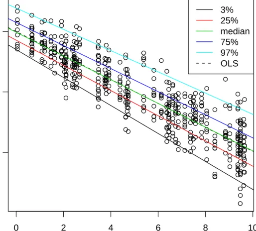
To construct an artificial example, we used 50 random uniform numbers on the in-terval (0,10) as the covariates. We then generated 5 observations at each covariate from the modelyi =β0+β1xi+ 1/11(11 +xi)²i, ²i ∼N(0,1) making 250

observa-tions in total. We choseβ0 = 10, β1 =−1. We then carried out quantile regression at 5 different quantiles, namely 5%, 25%, 50% 75% and 95%. We assumed no prior knowledge and used independentN(0,106_{) priors on all regression parameters and} Γ(10−3_,10−3_{) on all inverse scale parameters. Following the CODA analysis, we} ran the Gibbs sampler for 11,000 iterations and discarded the first 1,000 as burn in. Table 1 compares the posterior mean of the marginal distribution of β0(p)|y against the true quantile, given by 10 +Qp(N(0,1)) and compares the posterior

mean of β1(p)|y against the true quantile, given by 1/11Qp(N(0.1))−1. Figure

1 superimposes the quantile lines onto the data. Finally, table 2 compares the means of the 5 predictive quantile distributions of a new observation at xnew = 5.

0 2 4 6 8 10 0 5 10 x y 3% 25% median 75% 97% OLS

3.2

Length of stay as a performance indicator: quantile

regression approach

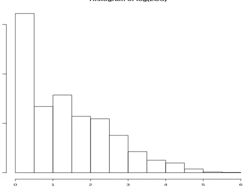
Length of stay in hospital (LOS) is a crucial variable for the quality of life of all patients and their families. Furthermore, it is the single most important component in the consumption of hospital resources. It is also very important for hospital planning since it is a direct determinant of the number of beds to be provided. Moreover, LOS is a frequent point of comparison between patients, hospitals and countries. We say that a patient’s LOS at the pth (0 < p < 1) quantile of a LOS distribution if his/her LOS is longer than the proportionpof the reference group of patients and shorter than the proportion (1−p). Thus, half of patients stay longer than the median patient and half stay shorter. Similarly, the quartiles divide the patient population into four segments with equal proportions of the reference population in each segment. The quintiles divide the population into five parts; the deciles into ten parts. Due to the strong skewness of the distribution (see Figure 2), we model the conditional quantiles of log(LOS) as a linear combination of admission age, admission method (a coded value dependent on how the patient was admitted) and gender (a binary variable taking 0 if the patient is female and 1 if the patient is male). We also fit a reduced model to see whether the gender of a patient has an effect on their log(LOS). We used informative priors on the regression parameters by assuming that all quantile planes would be parallel. We centred the corresponding normal distributions on the least squares solution (plus an additional Qp(N(0,1)) for the intercept

terms) with prior covariance matrix equal to the identity matrix. We placed uninformative priors on the inverse scale parameters. In order to see whether gender influences the log(LOS), we provide the approximate marginal likelihood ˆ

l(log(LOS)|Model). We also provide the deviance information criterion (DIC) (see Spiegelhalter et al., 2002), a statistic familiar to users of WinBUGS (Lunn

et al., 2000).

Like the previous section, 11,000 samples were generated with the first 1,000 samples rejected as burn in. Table 3 shows the posterior mean and 95% credible intervals for each of the 0.25, 0.5 and 0.75 quantile regression parameters. From this table, it can be seen that as the age of a patient increases, so does the log length of stay. This holds for all quantiles that were measured. What is also apparent is that as the “code” value associated with the method of admission increases, the log length of stay also increases. The maximum code value for this dataset was 28, which corresponds to a patient being transferred from another hospitals A&E, suggesting that this patient had the longest time in hospital. This was consistent across all measured quantiles.

At the median and 75th percentile, both the DIC and Bayes Factors favoured the full model. The Bayes Factors comparing the full model with the reduced model were 93.69 (median) and 343.78 (75th percentile) indicating strong dence on the Jeffreys (Jeffreys, 1961) that the full model was better. The evi-dence was not as strong at the 25th percentile with the DIC still preferring the

Figure 2: the histogram of LOS Histogram of log(LOS) log(LOS) Frequency 0 1 2 3 4 5 6 0 500 1000 1500

full model though not as convincingly. The Bayes Factor was 0.50 suggesting weak evidence for the reduced model. However, the 95% credible interval of the gender coefficient does not cross zero, suggesting that we should prefer the full model.

Table 3: Results of quantile regression analysis on log length of stay in hospital

p Model Covariates Marginal posterior mean 95% credible interval 0.25 Intercept -2.2037 (-2.4877,-1.8984) Admission age 0.0072 (0.0058,0.0085) Admission method 0.0989 (0.0842,0.1122) Gender -0.0580 (-0.1092,-0.0093) 0.50 Intercept -2.6639 (-3.0039,-2.3184) Admission age 0.0205 (0.0196,0.0213) Admission method 0.1268 (0.1107,0.1427) Gender -0.1166 (-0.1721,-0.0623) 0.75 Intercept -3.2594 (-3.6365,-2.8325) Admission age 0.0234 (0.0224,0.0244) Admission method 0.1832 (0.1640,0.2001) Gender -0.1411 (-0.2060,-0.0764)

Table 4: Comparison statistics for investigating whether length of stay depends on gender

p Model log ˆl(log(LOS)|Model) DIC

0.25 Full -7714.82 15377.58 Reduced -7714.13 15381.14 0.50 Full -7898.64 15745.73 Reduced -7903.18 15760.24 0.75 Full -8367.01 16682.80 Reduced -8372.85 16699.46

4

Discussions

We have introduced a PCG sampler for Bayesian quantile regression which uses simple conditional distributions to simulate the joint posterior distributions of all the unknown parameters in the regression models, including the latent vari-ables. We have also seen how it can be used to obtain marginal and predictive distributions and to carry out model testing for a particular quantile.

Using the location-scale mixture of normals representation of the AL distri-bution also permits more complicated quantile regression models to be analysed. In particular, the semiparametric model extension via nonparametric mixtures of AL distributions using a DP prior (section 2.6) allows the data to drive the shape of the error distribution. Nevertheless, Richardson (1999) pointed out that popular forms of priors tend to be those which have parameters that can be set straightforwardly and which lead to posterior with a relatively straightforward form.

Acknowledgements

The authors’ research were partially supported by an EPSRC doctorial Training Grant.

Appendix

Proof of Lemma

The proof proceeds in a similar fashion to the proof of Proposition 3.2.1. in Kotz et al. (2001).

If X ∼ AL(µ, τ, p), the moment generating function MX(t) = exp(tX) is

given by

MX(t) =

τ2_{p(1−p) exp(µt)}

(τ p−t)(τ(1−p) +t), −τ(1−p)< t < τ p (12) (Yu and Zhang, 2005).

LetY =q_{τ p(1}2ξ_−p)Z +_p1₍₁−₋2p_p)ξ+µ. Conditioning onξ, we have

MY(t) =E[exp(tY)] = E[E[exp(tY)|ξ]] = Z _∞ 0 τexp(−τ ξ)×exp ÃÃ 1−2p p(1−p)ξ+µ ! t ! MZ Ãs 2ξ τ p(1−p)t ! dξ. (13) Now since Z is standard normal, MZ(t) = exp(t2/2). Substituting this into

equation (13), we have MY(t) = τexp(µt) Z _∞ 0 exp à −ξ à τ− 1−2p p(1−p)t− 1 τ p(1−p)t 2 !! dξ (14)

= τexp(µt) Ã τ − 1−2p p(1−p)t− 1 τ p(1−p)t 2 !₋₁ = τ 2_{p(1−p) exp(µt)} p(1−p)τ2_{−(1−2p)τ t−t}2. (15) Note that the denominator in (15) factorises to (τ p−t)(τ(1−p) +t), which is the same as the denominator in (12). Hence MY(t) =MX(t), and therefore Y =d X.

Note also that the conditions for the integral in (14) to converge are exactly those for which MX(t) exists.

REFERENCES

Abrevaya, J. (2001), The Effects of Demographics and Maternal Behavior on the Distribution of Birth Outcomes, Empirical Economics, 26, 247–57.

Cade, B.S. and Noon, B.R. (2003), A gentle introduction to quantile regression for ecologists, Frontiers in Ecology and the Environment, 1, 412–420.

Casella, G. and George, E.I. (1992), Explaining the Gibbs Sampler,The American Statistician, 46, 167–174.

Chamberlain, G. (1994), Quantile Regression, Censoring and the Structure of Wages, Elsevier, New York.

Chen, L. and Yu, K. (2008), Automatic Bayesian Quantile Regression Curve, forthcoming in Statistics and Computing.

Chib, S. (1995), Marginal Likelihood from the Gibbs Output, Journal of the American Statistical Association, 90, 1313–1321.

Dunson, D.B. and Taylor, J. (2005), Approximate Bayesian inference for quan-tiles. Journal of Nonparametric Statistics, 17, 385–400.

Dunson,D.B., Pillai, N. and Park, J. (2007), Bayesian density regression, J. R. Statist. Soc. B, 69, 163-183.

Dunson, D.B., Reed, C. and Yu, K. (2009), Bayesian variable selection in quantile regression, Technical Report, Brunel University, UK.

Engle, R.F. & S. Manganelli (2004). CAViaR: Conditional autoregressive Value at Risk by regression quantile. Journal of Business and Economic Statistics, 22, 367–381.

Geman, S. and Geman, D. (1984), Stochastic Relaxation, Gibbs Distributions, and the Bayesian Restoration of Images, IEEE Transactions on Pattern Analysis and Machine Intelligence, 6, 721–741.

Geraci, M. and Bottai, M. (2007). Quantile regression for longitudinal data using the asymmetric Laplace distribution, Biostatistics, 8, 140–154.

Jeffreys, H. (1961), Theory of Probability. Clarendon Press: Oxford.

Koenker, R. and Hallock, K.F. (2001), Quantile regression, Journal of Economic Perspectives, 15, 143-156.

Koenker, R. (2005), Quantile Regression, Cambridge University Press, London. Kottas, A. and Gelfand, A.E. (2001), Bayesian semiparametric median regression modeling,Journal of the American Statistical Association, 96, 1458–1468

Kottas, A., and Krnjaji´c, M., (2009), Bayesian Semiparametric Modeling in Quantile Regression, To appear in Scandinavian Journal of Statistics.

Lancaster, T. and Jun, S.J. (2009), Bayesian quantile regression methods, forth-coming in Journal of Applied Econometrics.

Levin, J. (2001), For Whom the Reduction Counts: A Quantile Regression Anal-ysis of Class size on Scholastic Achievement, Empirical Economics, 26, 221–246. Lunn, D.J., Thomas, A., Best, N., and Spiegelhalter, D. (2000) WinBUGS – a Bayesian modelling framework: concepts, structure, and extensibility. Statistics and Computing, 10, 325–337.

Michael, J. R., Schucany, W.R. and Haas, R.W. (1976) Generating Random Variates Using Transformations with Multiple Roots, The American Statistician, 30, 88–90.

Min, I. and Kim, I. (2004), A Monte Carlo comparison of parametric and non-parametric quantile regressions, Applied Economic Letters 11, 71-74.

Plummer M., Best N., Cowles K. and Vines, K. (2008). coda: Output analysis and diagnostics for MCMC. R package version 0.13-3.

R Development Core Team (2008). R: A language and environment for statistical computing. R Foundation for Statistical Computing, Vienna, Austria. ISBN 3-900051-07-0, URL http://www.R-project.org.

Richardson, S. (1999) “Contribution to the Discussion of Walker et al., Bayesian Nonparametric Inference for Random Distribution and Related Functions” J. R. Statist. Soc. B, 61, 485–527.

Spiegelhalter, D.J., Best, N.G., Carlin, B.P. and van der Linde A. (2002) Bayesian measures of model complexity and fit (with discussion), J Roy Statist Soc B,64, 583–640.

compu-tation and simulation, 73, 659–674

van Dyk, D. A. and Park, T. (2008). Partially Collapsed Gibbs Samplers: Theory and Methods. Journal of the American Statistical Association 103, 790–796. Yu, K. and Moyeed, R.A. (2001), Bayesian Quantile Regression, Statistics and Probability Letters, 54, 437–447.

Yu, K., Lu,Z. and Stander,J. (2003), Quantile regression: Applications and cur-rent research areas, The Statistician, 52, 331–350.

Yu, K. and Stander, J. (2007), Bayesian Analysis of a Tobit Quantile Regression Model, Journal of Econometrics, 137, 260–276

Yu, K. and Zhang, J. (2005), A three-parameter asymmetric laplace distribution and its extensionCommunications in Statistics - Theory and Methods, 34, 1867– 1879.

Yu, K., Dunson, D.B. and Reed, C. (2009), Bayesian skewed Lesso, Technical Report, Brunel University, UK.