Program for statistical comparison of
histograms
S. Bityukov (IHEP, INR), N. Tsirova (NPI MSU)
Scope
• Introduction
• Statistical comparison of two histograms
• Normalized significance
• Example
• “Distance measure”
• Internal resolution of the method
• Script stat analyzer.C
• Missing ET: large difference between histograms • PT light jet: only statistical difference
• Output of the script
Introduction
Sometimes we have two histograms and are faced with the question: Are the realizations of random variables in the form of these histograms taken from the same statistical population?
There are many approaches for comparison of two histograms: Kolmogorov-Smirnov test, Cramer-von-Mises test, Anderson-Darling test, Likelihood ratio test for shape and for slope, ... .
The review on this subject is in the paper “Testing Consistency of Two Histograms” by F. Porter.
http://arxiv.org/abs/0804.0380
Usually, a special test-statistic is used for comparing the two histograms
Statistical comparison of two histograms
A method, which uses the distribution of test-statistics
for each bin of histograms, is proposed in note arXiv:1302.2651. These test-statistics obeys the distribution close to
standard normal distribution if both histograms are obtained from the same statistical population by the same analyzer of data. Correspondingly, the joint dis-tribution must be close to standard normal distribu-tion.
For example, if we consider observed values which are produced by the same Poisson flow of events dur-ing equal independent time ranges then a test statistic
ˆ Sc12 = 2· ( √ ˆ ni1 − √ ˆ ni2),
where nˆi1 is a number events in bin i of histogram
1, nˆi2 is a number events in bin i of histogram 2, is
the test statistic of such type. It is shown in paper PoS(ACAT08)118.
Often test-statistics of such type are named as “sig-nificances of a deviation” or “sig“sig-nificances of an en-hancement”.
Normalized significance
Let us consider a model with two histograms where the random variable in each bin obeys the normal dis-tribution ϕ(x|nik) = 1 √ 2πσik e− (x−nik)2 2σ2 ik . (1)
Here the expected value in the bin i is equal to nik and
the variance σn2ik is also equal to nik. k is the histogram
number (k = 1,2).
Let integral in the histogram 1 equals N1 and
inte-gral in the histogram 2 equals N2 (for example, if we
have different integrated luminosity in experiments). We define the normalized significance as
ˆ Si(K) = ˆ ni1 − Knˆi2 r ˆ σn2i1 + K2σˆn2i2. (2)
Here nˆik is an observed value in the bin i of the
his-togram k, σˆn2ik = ˆnik and coefficient of normalization
K = N1 N2
Example
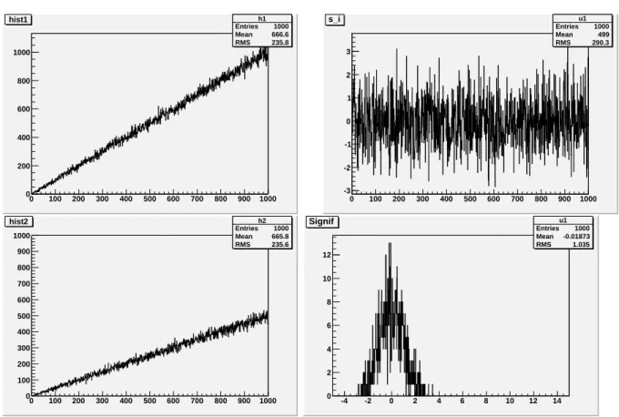
h1 Entries 1000 Mean 666.6 RMS 235.8 0 100 200 300 400 500 600 700 800 900 1000 0 200 400 600 800 1000 h1 Entries 1000 Mean 666.6 RMS 235.8 hist1 u1 Entries 1000 Mean 499 RMS 290.3 0 100 200 300 400 500 600 700 800 900 1000 -3 -2 -1 0 1 2 3 u1 Entries 1000 Mean 499 RMS 290.3 s_i h2 Entries 1000 Mean 665.8 RMS 235.6 0 100 200 300 400 500 600 700 800 900 1000 0 100 200 300 400 500 600 700 800 900 1000 h2 Entries 1000 Mean 665.8 RMS 235.6 hist2 u1 Entries 1000 Mean -0.01873 RMS 1.035 -4 -2 0 2 4 6 8 10 12 14 0 2 4 6 8 10 12 u1 Entries 1000 Mean -0.01873 RMS 1.035 SignifFigure 1: Triangle distributions (K = 2, M = 1000): the observed values ˆni1 in the
first histogram (left,up), the observed values ni2 in the second histogram (left, down),
observed normalized significances ˆSi bin-by-bin (right, up), the distribution of observed
normalized significances (right, down).
The example with histograms produced from the same events flow during unequal independent time ranges shows that the standard deviation (RMS in the ROOT notation) of the distribution in the picture (right, down) can be used as estimator of the statisti-cal difference between histograms (this distribution is close to standard normal distribution in our example).
“Distance measure”
The RMS as a “distance measure” in our case has a clear interpretation (in fact, we set a scale of this “differmeter”):
• RM S = 0 – histograms are identical;
• RM S ∼ 1 – both histograms are obtained (by the
using independent samples) from the same parent distribution;
• RM S >> 1 – histograms are obtained from
differ-ent pardiffer-ent distributions.
An accuracy (internal resolution) of the method
de-pends on the number of bins M in histograms and on
the normalized coefficient K. The accuracy can be
estimated via Monte Carlo experiments.
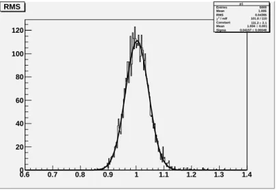
p1 Entries 5000 Mean 1.005 RMS 0.04395 / ndf 2 χ 101.8 / 110 Constant 111.2 ± 2.1 Mean 1.004 ± 0.001 Sigma 0.04157 ± 0.00048 0.6 0.7 0.8 0.9 1 1.1 1.2 1.3 1.4 0 20 40 60 80 100 120 p1 Entries 5000 Mean 1.005 RMS 0.04395 / ndf 2 χ 101.8 / 110 Constant 111.2 ± 2.1 Mean 1.004 ± 0.001 Sigma 0.04157 ± 0.00048 RMS
Figure 2: Distribution of RMS for 5000 comparisons of histograms (triangle distribution,
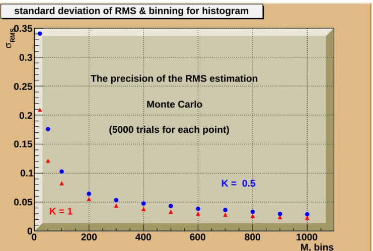
Internal resolution of the method
The dependencies of the internal resolution on the
bin numbers M and on the value of coefficient of
nor-malization K are shown in Fig. 3.
M, bins 0 200 400 600 800 1000 RMS σ 0 0.05 0.1 0.15 0.2 0.25 0.3 0.35 K = 1 K = 0.5 The precision of the RMS estimation
Monte Carlo
(5000 trials for each point) standard deviation of RMS & binning for histogram
Figure 3: The dependence of the standard deviation of RMS on number of binsM. This
Script stat analyzer.C
Two input files (*.root) with a set of TH1D his-tograms to compare.
User should indicate which histograms he/she wants to compare.
Processing:
– calculate mean value, RMS and p-value for each pair of histograms;
– sort variables by RMS in descending order; – print sorted results
(variable – p-value – RMS – mean). Output:
– to screen; – to text file.
Commands for start-up of script in ROOT root[0] .L stat analyzer.C++
Missing
E
T: large difference between
histograms
0 10 20 30 40 50 60 70 80 90 100 0.01 0.02 0.03 0.04 0.05 0.06 0.07 0.08MET, signal Entries s1 20
Mean 54.33 RMS 31.1 0 10 20 30 40 50 60 70 80 90 100 -15 -10 -5 0 5 10 15 s1 Entries 20 Mean 54.33 RMS 31.1 Significances, bin-by-bin s_i 0 10 20 30 40 50 60 70 80 90 100 0.01 0.02 0.03 0.04 0.05 0.06 0.07 0.08 0.09
MET, anomalous Wtb coupling
d1 Entries 20 Mean 1.993 RMS 10.74 -20 -15 -10 -5 0 5 10 15 20 0 0.5 1 1.5 2 2.5 3 3.5 4 d1 Entries 20 Mean 1.993 RMS 10.74 Distribution of significances p-value = 1.7231041929895835e-32 Signif
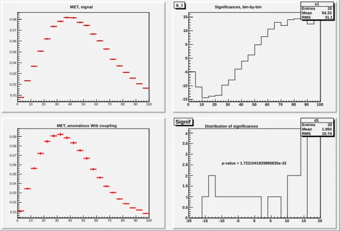
Figure 4: MET: the observed values in the first histogram (left,up), the observed values in the second histogram (left, down), observed normalized significances bin-by-bin (right, up), the distribution of observed normalized significances (right, down).
Let us consider the distributions of the probability
(with errors) of the missing ET to be in corresponding
bin of histogram in the case of registration of Standard Model events and the events which are produced due to the presence of anomalous Wtb coupling. The com-parison of these distributions is shown in Fig. 4 (RMS
P
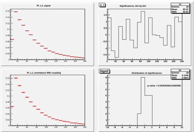
Tlight jet: only statistical difference
40 60 80 100 120 140 160 180 0 0.02 0.04 0.06 0.08 0.1 0.12 0.14 0.16 Pt_LJ, signal Entries s1 20 Mean 83.32 RMS 55.64 0 20 40 60 80 100 120 140 160 180 -1.5 -1 -0.5 0 0.5 1 1.5 s1 Entries 20 Mean 83.32 RMS 55.64 Significances, bin-by-bin s_i 40 60 80 100 120 140 160 180 0 0.02 0.04 0.06 0.08 0.1 0.12 0.14 0.16 Pt_LJ, anomalous Wtb coupling d1 Entries 20 Mean 0.1446 RMS 0.9824 -10 -8 -6 -4 -2 0 2 4 6 8 10 0 1 2 3 4 5 6 7 8 d1 Entries 20 Mean 0.1446 RMS 0.9824 Distribution of significances p-value = 0.54364536413492959 SignifFigure 5: Pt LJ: the observed values in the first histogram (left,up), the observed values in the second histogram (left, down), observed normalized significances bin-by-bin (right, up), the distribution of observed normalized significances (right, down).
The case of the absence of the difference between distributions for the production of single top quark in frame of SM and model with anomalous Wtb coupling is shown in Fig. 5 for Pt distribution of jet from light
Output of the script
Conclusions
• We discussed the possible tool for comparison of
histograms in frame of the ROOT system (script stat analyzer.C).
• This tool very easy in use and very easy to
under-stand the results.
• This tool can be used in tasks of monitoring of the
equipment. In this moment the method is used for choice of the most significant variables in mul-tivariate analysis.
• This tool requires the additional development (now
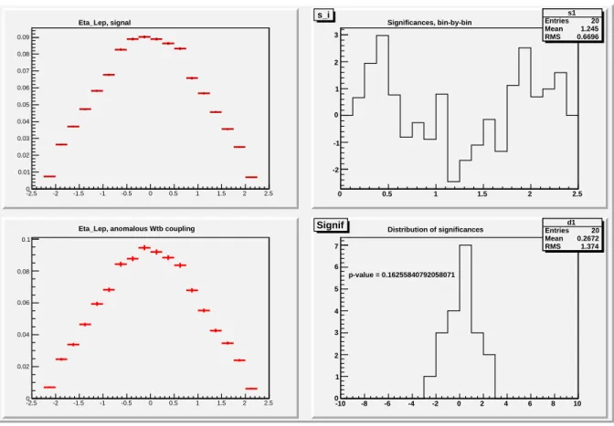
η
of lepton: the difference exits
-2.5 -2 -1.5 -1 -0.5 0 0.5 1 1.5 2 2.5 0 0.01 0.02 0.03 0.04 0.05 0.06 0.07 0.08 0.09 Eta_Lep, signal s1 Entries 20 Mean 1.245 RMS 0.6696 0 0.5 1 1.5 2 2.5 -2 -1 0 1 2 3 s1 Entries 20 Mean 1.245 RMS 0.6696 Significances, bin-by-bin s_i -2.5 -2 -1.5 -1 -0.5 0 0.5 1 1.5 2 2.5 0 0.02 0.04 0.06 0.08 0.1Eta_Lep, anomalous Wtb coupling Entries d1 20 Mean 0.2672 RMS 1.374 -10 -8 -6 -4 -2 0 2 4 6 8 10 0 1 2 3 4 5 6 7 d1 Entries 20 Mean 0.2672 RMS 1.374 Distribution of significances p-value = 0.16255840792058071 Signif
Figure 7: Eta Lep: the observed values in the first histogram (left,up), the observed values in the second histogram (left, down), observed normalized significances bin-by-bin (right, up), the distribution of observed normalized significances (right, down).
The case of small difference between the histograms is shown in Fig. 7 (RMS = 1.37, Mean = 0.29).