Interval Estimate for Specific Points in Polynomial Regression

Journal of Computing and Information Technology - CIT 13, 2005, 4, 287–291 287

Interval Estimate for Speci

fi

c

Points in Polynomial Regression

Katarina Ko

smelj

ˇ

_{, Andrej Blejec}

_{and Anton Cedilnik}

2_{National Institute of Biology, Ljubljana, Slovenia}

This paper presents the interval estimate for specific points in polynomial regression: zero of a linear regres-sion, abscissa of the extreme of a quadratic regresregres-sion, abscissa of the inflection point of a cubic regression. Two different approaches are under study. An application of these two approaches based on quadratic regression in presented: interval estimate for the plant density giving optimal yield of maize is under consideration.

Keywords: zero of a linear regression, extreme of a quadratic regression, density of the ratio of two normal variables.

1. Introduction

Consider a general polynomial regression E(Yjx) =β0+β1x+:::+βmx

m_{,m 1. Let}

us defineZ = ;Bm ;1

=(mBm). Form=1,Z is

an estimator for the zero of a linear regression. Form=2,Zis an estimator for the abscissa of

the extreme of a quadratic regression, and for m=3,Z is an estimator for the abscissa of the

inflection point of a cubic regression.

These points are often of research interest, in particular in biological and agricultural setting. Experimenters are interested in the point and in-terval estimate ofZ. In this context, we consider these points asspecific pointsof polynomial re-gression and focus our attention on the distribu-tion ofZ. In the last section, we consider the data from an agricultural experiment on maize. The experimenters were interested in the point and interval estimate of the plant density giving optimal yield.

2. Distribution of the Ratio of Jointly Normal Variables

Under standard regression assumptions,Zis ex-pressed as the ratio of two normally distributed and dependent variables. From the standard probability literature 3], it is known that the

ratio of two centred normal variables: Z =X=Y

X Y]

T _:N

(µX =µY =0 σXσY ρ 6=1)

is a non-centered Cauchy variable,

Z :C a=ρ

σX σY b= σX σY q

1;ρ

2

:

In4]and2], authors discussed the general

sit-uation. Independently of Hinkley, we 1]

fol-lowed the same procedure as he did, but we expressed the density differently, as a product of two parts:

pZ(z)=

σXσY

p

1;ρ

2

π(σ

2

Yz2;2ρσXσYz+σ

2 X) exp ; 1

2 supR

2

+

p

2π R

Φ(R)exp ;

1 2

h

supR2;R

2

i

(1)

where:

R=R(z)= µX σX ;ρ µY σY z;

ρµX σX ; µY σY σX σY p

1;ρ

2

s

z2

;2ρ

σX

σYz

+

σX

σY

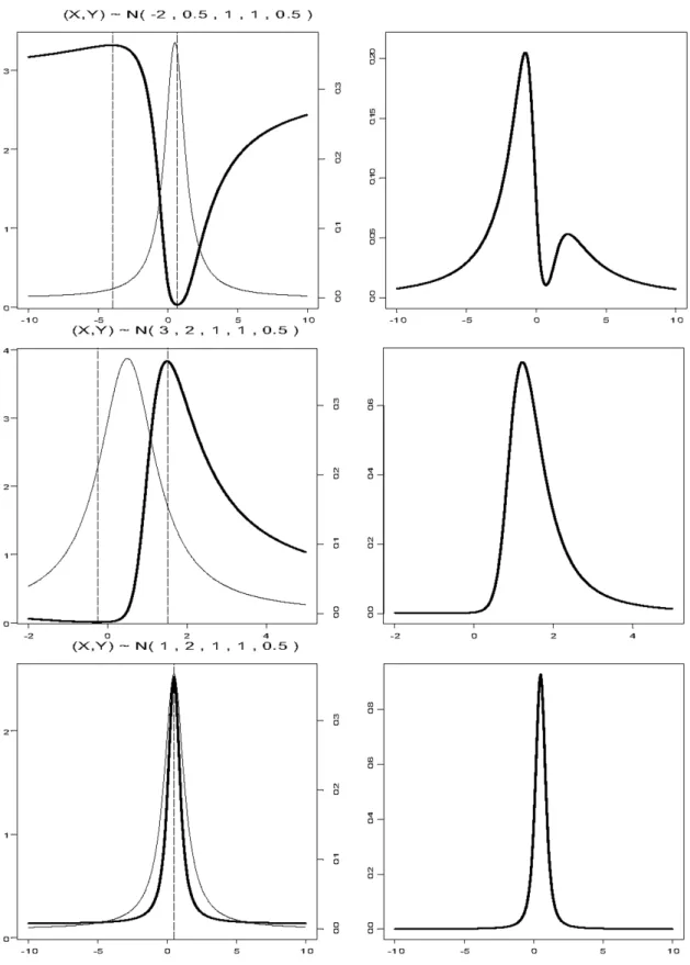
Fig. 1.On the left, the standard Cauchy part(thick line)and the deviant part(thin line)are presented; the scale for

Interval Estimate for Specific Points in Polynomial Regression 289

supR2=const=

µX

σX

2 ;2ρ

µX σX µY σY + µY σY 2

1;ρ

2

supR2;R

2 = µX σX σX σY ; µY

σYz

2

z2

; 2ρ

σX

σYz

+

σX

σY

2 :

The first factor in(1), thestandard part, is the

density for a non-centred Cauchy,

C a =ρ

σX σY b= σX σY q

1;ρ

2

;

it is independent of the expected valuesµX and

µY. The second factor, the deviant part, is a

rather complicated function of z. The asymp-totic behaviour ofpZ(z)is the same as that of the

Cauchy density, consequently E(Z) and other

moments do not exist. We need four parame-ters to describe the distribution:ρ, µX

σX,

µY

σY and

σX

σY. In general,pZ

(z)is bimodal.

We studied the density originating from the distribution N (µX,µY, 1, 1, 0.5) for

differ-ent values of µX and µY. The standard part

is C

0:5; p

3=2

, it is symmetric around its median 0.5. Different values for µX and µY

determine different shapes of the deviant part. Figure 1 displays three possible shapes of the density: evident bimodality (above), the

de-viant part prevails(in the middle); the Cauchy

and the deviant part are superimposed and the density is unimodal(below).

3. Application

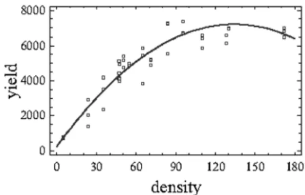
In an agricultural setting in Slovenia, experi-menters studied the impact of the plant density on the yield of maize. In a field experiment, 15 different plant densities were included, each in four replications. The yield was the variable of interest. The experimenters were interested in the point and interval estimate for the plant density providing optimal yield.

Fig. 2. Yield of maizekg per ha)]depending on plant

density1000plants per ha]. The thick line represents

the graph for quadratic polynomialfitted to the data.

The graph(Figure 2)and the analysis(Table 1)

show that quadratic polynomial fits the data very well. The point estimate for the optimal density is z = 103:588=(20:385395) = 134:4,

how-ever the interval estimate requires more elabo-rate consideration.

Parameter Estimate St. Error T-Statistic P-Value

b0 249.193 321.881 0.77418 0.4432

b1 103.588 8.34109 12.419 0.0000

b2 -0.385395 0.046127 -8.35504 0.0000 R2=88.5 %.

Table 1. Quadratic Regression Analysis. Dependent variable: yield per ha, independent variable:

plant density.

We obtained the estimates for the bivariate nor-mal distribution from Table 1 and correlation matrix of the regression estimates:

;b1=;103:6 2b2 =0:771 s(;b1)=8:341,

s(2b2)=0:0923 cor(;b12b2)=0:961.

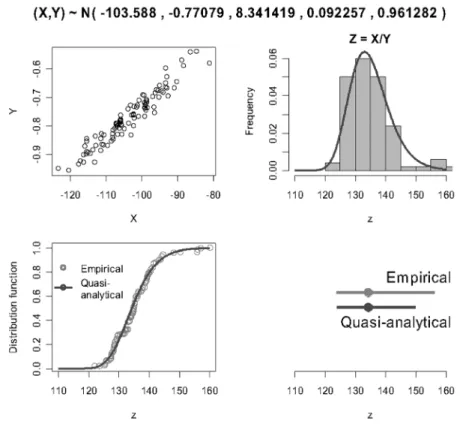
These values were plugged into the computer program as if they were the true values of the bivariate normal distribution (quasi-analytical

approach). Figure 3 shows the Cauchy part (first factor) and the deviant part (second

fac-tor), the probability density and the distribution

Fig. 3.Cauchy part(First factor, above left)and the deviant part(Second factor, above right)for the bivariate normal

distribution, probability density(below left)and distribution function(below right). Interval estimate for optimal

plant density is obtained numerically from the distribution function.

Fig. 4.Scatterplot of 100 values generated from the bivariate normal distribution(left above), histogram of the ratios

and the density obtained from the quasi-analytical approach(right above). The two distribution functions obtained

Interval Estimate for Specific Points in Polynomial Regression 291

As an alternative approach we generated a ran-dom sample from the bivariate normal distribu-tion obtained above(empirical approach). Two

sample sizes were considered, 100 and 1000. Figure 4 presents the scatterplot of 100 gener-ated values, the histogram for the ratios fitted by the density obtained from the quasi-analytical approach. The two distribution functions were obtained numerically and were used to acquire the two interval estimates.

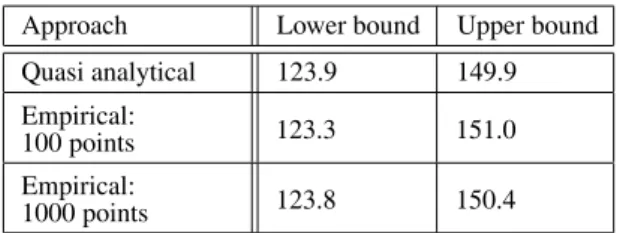
We present the final results for the interval esti-mate in Table 2. The comparison of the intervals shows minor discrepancy with quasi-analytical approach, in particular for the sample size 1000.

Approach Lower bound Upper bound Quasi analytical 123.9 149.9 Empirical:

100 points 123.3 151.0 Empirical:

1000 points 123.8 150.4

Table 2.Interval estimate for optimal plant density obtained by two different approaches(see text).

4. Conclusion

This paper presents two different approaches to obtain the interval estimate for a ratio of two normally distributed and dependent variables. The quasi-analytical approach is based on the derived probability density, the regression esti-mates are taken as true values of the parameters of the bivariate normal distribution. The second approach is empirical, random samples from the corresponding distribution are generated.

5. Acknowledgments

We thank Prof. dr. Anton Tajnˇsek, University of Ljubljana, for the data.

References

1] A. CEDILNIK, K. KOSMELJˇ , A. BLEJEC,(2004). The

Distribution of the Ratio of Jointly Normal Vari-ables.Metodoloski zvezkiˇ . Vol.1, No. 1, 2004, pp. 99–108.

2] D. V. HINKLEY,(1969). On the ratio of two

corre-lated normal random variables.Biometrika,56, 3, pp. 635–639.

3] N. L. JOHNSON, S. KOTZ AND N. BALAKRISHNAN, (1994). Continuous Univariate Distributions. 1.

John Wiley and Sons.

4] G. MARSAGLIA,(1965). Ratios of normal variables

and ratios of sums of uniforms variables.JASA, 60, pp. 163–204.

Recived:June, 2005.

Accepted:October, 2005.

Contact address:

Biotechnical Faculty University of Ljubljana Ljubljana Slovenia

Katarina.Kosmelj@bf.uni-lj.si

Andrej Blejec National Institute of Biology Ljubljana Slovenia

Andrej.Blejec@nib.si

Anton Cedilnik Biotechnical Faculty University of Ljubljana Ljubljana Slovenia

Anton.Cedilnik@bf.uni-lj.si

KATARINAKOˇSMELJis a professor of statistics at Biotechnical Faculty, University of Ljubljana. She is specialized in design and analysis of experiments and data analysis. Her area of work is applied biostatistics.

ANDREJBLEJECis an assistant professor of statistics and computer sci-ence at Biotechnical Faculty, University of Ljubljana. Currently he works as a statistician at the National Institute of Biology in Ljubl-jana. His main interest is computational statistics, data visualization and statistical simulation systems for statistics education.

ANTONCEDILNIKis an associate professor of mathematics at