A short note on quantile and expectile estimation in unequal probability samples

(1)

Survey Methodology

ISSN 1492-0921

by Linda Schulze Waltrup and Göran Kauermann

A short note on quantile and expectile

estimation in unequal probability

samples

(2)

Standard table symbols

The following symbols are used in Statistics Canada publications:

. not available for any reference period .. not available for a specific reference period ... not applicable

0 true zero or a value rounded to zero

0s_{value rounded to 0 (zero) where there is a meaningful}

distinction between true zero and the value that was rounded

p_preliminary r_revised

x suppressed to meet the confidentiality requirements of the Statistics Act

E_{use with caution}

F too unreliable to be published

* significantly different from reference category (p < 0.05)

How to obtain more information

For information about this product or the wide range of services and data available from Statistics Canada, visit our website,

www.statcan.gc.ca. You can also contact us by

email at[email protected]

telephone, from Monday to Friday, 8:30 a.m. to 4:30 p.m., at the following toll-free numbers:

• Statistical Information Service 1-800-263-1136

• National telecommunications device for the hearing impaired 1-800-363-7629

• Fax line 1-877-287-4369

Depository Services Program

• Inquiries line 1-800-635-7943

• Fax line 1-800-565-7757

Published by authority of the Minister responsible for Statistics Canada © Minister of Industry, 2016

Cette publication est aussi disponible en français.

Note of appreciation

Canada owes the success of its statistical system to a long-standing partnership between Statistics Canada, the citizens of Canada, its businesses, governments and other institutions. Accurate and timely statistical information could not be produced without their continued co-operation and goodwill.

Standards of service to the public

Statistics Canada is committed to serving its clients in a prompt, reliable and courteous manner. To this end, Statistics Canada has developed standards of service that its employees observe. To obtain a copy of these service standards, please contact Statistics Canada toll-free at 1-800-263-1136. The service standards are also published on www.statcan.gc.ca under “Contact us” > “Standards of service to the public.”

(3)

Vol. 42, No. 1, pp. 179-187

Statistics Canada, Catalogue No. 12-001-X

1. Linda Schulze Waltrup, Business Administration and Social Sciences, Ludwig Maximilian University of Munich, Ludwigstraße 33, 80539 Munich, Germany. E-mail: [email protected]; Göran Kauermann, Business Administration and Social Sciences, Ludwig Maximilian University of Munich, Ludwigstraße 33, 80539 Munich, Germany. E-mail: [email protected].

A short note on quantile and expectile estimation in unequal

probability samples

Linda Schulze Waltrup and Göran Kauermann

1

Abstract

The estimation of quantiles is an important topic not only in the regression framework, but also in sampling theory. A natural alternative or addition to quantiles are expectiles. Expectiles as a generalization of the mean have become popular during the last years as they not only give a more detailed picture of the data than the ordinary mean, but also can serve as a basis to calculate quantiles by using their close relationship. We show, how to estimate expectiles under sampling with unequal probabilities and how expectiles can be used to estimate the distribution function. The resulting fitted distribution function estimator can be inverted leading to quantile estimates. We run a simulation study to investigate and compare the efficiency of the expectile based estimator.

Key Words: Quantiles; Expectiles; Probability proportional to size; Design-based; Auxiliary variable; Distribution

function.

1 Introduction

Quantile estimation and quantile regression have seen a number of new developments in recent years with Koenker (2005) as a central reference. The principle idea is thereby to estimate an inverted cumulative distribution function, generally called the quantile function _Q

 

_ ₌ _F1

 

_ _for _{ }

 

_{0,1 ,}_{where the}

0.5 quantile Q

 

0.5 , the median, plays a central role. For survey data tracing from an unequal probability sample with known probabilities of inclusion Kuk (1988) shows how to estimate quantiles taking the inclusion probabilities into account. The central idea is to estimate a distribution function of the variable of interest and invert this in a second step to obtain the quantile function. Chambers and Dunstan (1986) propose a model-based estimator of the distribution function. Rao, Kovar and Mantel (1990) propose a design-based estimator of the cumulative distribution function using auxiliary information. Bayesian approaches in this direction have recently been proposed in Chen, Elliott, and Little (2010) and Chen, Elliott, and Little (2012).

Quantile estimation results from minimizing an L₁ loss function as demonstrated in Koenker (2005). If the L₁ loss is replaced by the L₂ loss function one obtains so called expectiles as introduced in Aigner, Amemiya and Poirier (1976) or Newey and Powell (1987). For  

 

0,1 , this leads to the expectile function M

 

 which, like the quantile function Q

 

 , uniquely defines the cumulative distribution function ( )F y . Expectiles are relatively easy to estimate and they have recently gained some interest, see e.g., Schnabel and Eilers (2009), Pratesi, Ranalli, and Salvati (2009), Sobotka and Kneib (2012) and Guo and Härdle (2013). However since expectiles lack a simple interpretation their acceptance and usage in statistics is less developed than quantiles, see Kneib (2013). Quantiles and expectiles are connected in that a unique and invertible transformation function h_y : 0,1

 



 

0,1 exists so that M h



 





= Q

 

 , see Yao and Tong (1996) and De Rossi and Harvey (2009). This connection can be used to estimate quantiles

(4)

180 Schulze Waltrup and Kauermann: A short note on quantile and expectile estimation in unequal probability samples

from a set of fitted expectiles. The idea has been used in Schulze Waltrup, Sobotka, Kneib and Kauermann (2014) and the authors show empirically that the resulting quantiles can be more efficient than empirical quantiles, even if a smoothing step is applied to the latter (see Jones 1992). An intuitive explanation for this is that expectiles account for all the data while quantiles based on the empirical distribution function only take the left (or the right) hand side of the data into account. That is, the median is defined by the 50% left (or 50% right) part of the data while the mean (as 50% expectile) is a function of all data points. In this note we extend these findings and demonstrate how expectiles can be estimated for unequal probability samples and how to obtain a fitted distribution function from fitted expectiles.

The paper is organized as follows. In Section 2 we give the necessary notation and discuss quantile regression in unequal probability sampling. This is extended in Section 3 towards expectile estimation. Section 4 utilizes the connection between expectiles and quantiles and demonstrates how to derive quantiles from fitted expectiles. Section 5 demonstrates in simulations the efficiency gain in quantiles derived from expectiles and a discussion concludes the paper in Section 6.

2 Quantile estimation

We consider a finite population with N elements and a continuous survey variable Y. We are interested in quantiles of the cumulative distribution function

 





=1 = N 1 i i F y



Y  y N and define as

 





=1

= inf arg min

N i i q i Q   w_ Y  q Y  q  



 (2.1)

the Quantile function of Y (see Koenker 2005), where

 

= for > 0 1 for 0. w_     _     

The “inf” argument in (2.1) is required in finite populations since the “arg min” is not unique. We draw a sample from the population with known inclusion probabilities ,_i = 1,i , .N Denoting by y₁,,y_n the resulting sample, we estimate the quantile function by replacing (2.1) through its weighted sample version

 

,

=1

1 ˆ _{= inf arg min} n

N _q j j

j j

Q  _ w_ y q _







 (2.2)

with w__,_j = w_



y_j q



as defined above. It is easy to see that the sum in (2.2) is a design-unbiased estimate for the sum in Q

 

 given in (2.1). Nonetheless, because we take the “arg min” it follows that

 

ˆ

N

Q  is not unbiased for Q

 

 . We therefore look at consistency statements for Qˆ_N

 

 as follows. Let

 

=





i i i R q w y q y  q and

 

:= 1

 

. N i i R q R q N



(5)

We draw a sample from R q_i

 

, = 1,i ,N and assume we apply a consistent sampling scheme in that

 

=1 1 1 := n n j j j r q r q N





is design-consistent for R_N

 

q , where r q_j

 

denotes the sample of R q_i

 

. Note that r q_j

 

and hence

 

,

n

r q R q_i

 

and R_N

 

q also depend on  which is suppressed in the notation for readability. Let q₀ be the minimum of R_N

 

q which is not necessarily unique due to the finite structure of the population. We can take the “inf” argument, i.e., q₀ = inf arg min



R_N

 

q



, but for simplicity we assume a superpopulation model (see Isaki and Fuller 1982) by considering the finite population to be a sample from an infinite superpopulation. In the latter we assume that survey variable Y has a continuous cumulative distribution function so q₀ results in a unique  quantile. We get for  > 0

 







0 0





 

0



0





=1 1 1 < < 0 . n n n j j j j P r q r q P r q r q N      _    _  





Note that the argument in the probability statement is a design-consistent estimate for R_N

 

q₀ 



0



,

N

R q   which is less than zero since q₀ is the minimum of R_N

 

 . Hence, the probability tends to one in the sense of design consistency defined in Isaki and Fuller (1982). The same holds of course for

< 0.

 With this statement we may conclude that the estimated minimum ₀

 

=1

ˆ = arg min n 1

j j j

q



 r q

is a design-consistent estimate for q₀ so that Qˆ_N

 

 in (2.2) is in turn design-consistent for Q_N

 

 . It is easily shown that Qˆ_N

 

 is the inverse of the normed weighted cumulative distribution function

 

=1





=1 1 ˆ _:= 1 n j j j N n j j y y F y   



using the same notation as in Kuk (1988). Note that Fˆ_N

 

y is the Hajek (1971) estimate of the cumulative distribution function (see also Rao and Wu 2009) and as such not a Horvitz-Thompson estimate. As a consequence Qˆ_N

 

 is not design-unbiased. Nonetheless, Fˆ_N

 

y is a valid distribution function, and hence it can be considered as normalized version of the Lahiri or Horvitz-Thompson estimator of the distribution function (see Lahiri 1951) which is denoted by

 





=1 1 ˆ _:= n ₁ ₁ _. L j j j F y y y N



 

Kuk (1988) proposes to replace Fˆ_L

 

 with alternative estimates of the distribution function: Instead of estimating the distribution function itself he suggests to estimate the complementary proportion Sˆ_R

 

y which then leads to the estimate Fˆ_R

 

y defined through

 





=1 1 ˆ ˆ _{= 1} _{= 1} n ₁ ₁ _> _. R R j j j F y S y y y N  





(6)

Resulting directly from these definitions we can express Fˆ_R

 

 in terms of Fˆ_N

 

 through

=1 =1 1 1 ˆ _{= 1} ₁ ˆ _and ˆ ₌ ˆ _. n j n j R j L L N j F F F F N N  



 



(2.3)

Kuk (1988) shows that, under sampling with unequal probabilities, estimation of the median derived from ˆ

R

F outperforms median estimates derived from ˆF_N and ˆF_L in terms of mean squared estimation error. Note that the estimators ˆ ,F_N ˆF_L and ˆF_R coincide in the case of simple random sampling without replacement where _j =  = n N.

3 Expectile estimation

An alternative to quantiles are expectiles. The expectile function M

 

 is thereby defined by replacing the L₁ loss in (2.1) by the L₂ loss leading to

 



 



2 =1 = arg min . N i i m i M  _ w_ Y  m Y  m _ 



 (3.1)

Note that M

 

 is continuous in  even for finite populations. Moreover M

 

0.5 equals the mean value

=1

= N _i .

i

Y



Y N Using the sample y₁,,y_n with inclusion probabilities ₁,,_n we can estimate

 

M  by replacing the sum in (2.2) by its sample version, i.e.,

 





2 , =1 1 ˆ _{= arg min} n j j m j j M  _ w_ y  m _  





with w__,_j as defined above. It is easy to see that the sum in Mˆ

 

 is a design-unbiased estimate for the sum in M

 

 . The estimate itself is however not design-unbiased like for the quantile function above. However the same arguments as for Q_N

 

 in (2.2) may be used to establish design-consistency.

4 From expectiles to the distribution function

Both, the quantile function Q

 

 and the expectile function M

 

 uniquely define a distribution function F

 

. . While Q

 

 is just the inversion of F

 

. the relation between M

 

 and F

 

. is more complicated. Following Schnabel and Eilers (2009) and Yao and Tong (1996), we have the relation

 







 





 



 











 







 





1 0.5 = , 1 1 G M M G M M F M F M                (4.1)

where G m

 

is the moment function defined through

 

= N₌₁ _i1



_i



.

i

G m



Y Y  m N Expression (4.1) gives the unique relation of function M

 

 to the distribution function F

 

. . The idea is now to solve (4.1) for F

 

. , that is to express the distribution F

 

. in terms of the expectile function M

 

. . Apparently,

(7)

this is not possible in analytic form but it may be calculated numerically. To do so, we evaluate the fitted function Mˆ

 

 at a dense set of values 0 < ₁ < ₂< _L < 1 and denote the fitted values as

 

ˆ ˆ =_l _l .

m M  We also define left and right bounds through mˆ_o = mˆ₁ c₀ and mˆ_L_₁ = mˆ_L  c_L_₁, where

0

c and c_L are some constants to be defined by the user. For instance, one may set c₀ = mˆ₂  mˆ₁ and

1 = ˆ ˆ 1.

L L L

c _ m  m _ By doing so we derive fitted values for the cumulative distribution function F

 

. at ˆm_l which we write as ˆ := ˆ ˆ

 

= l₌₁ˆ

l l j j

F F m



 for non-negative steps ˆ _j 0, = 1,j ,L with



L_j₌₁ ˆ_j 1. We define ˆ ₁ = 1 L₌₁ˆ

L l l

 



 to make Fˆ .

 

a distribution function. Assuming a uniform distribution between the dense supporting points ˆm_l we may express the moment function G

 

. by simple stepwise integration as

 

=1 ˆ ˆ ˆ _:= ˆ _ˆ ₌ m_l ₌ˆ l _, l l j l j G G m x dF x d 







where dˆ_j =



mˆ_j  mˆ_j_₁



2 with the constraint that Gˆ_L₁ = Mˆ

 

0.5 and Mˆ 0.5 =

 









=1 =1 1 .

n n

j j j

j y  j 



With the steps ˆ , = 1,_l l ,L we can now re-express (4.1) as





 





=1 =1 =1 =1 ˆ ˆ ˆ ˆ ˆ 1 0.5 ˆ = , = 1, , , ˆ ˆ 1 1 l l j j j j j j l l l j j j j d M d m l L       _  _{ }         _  _{ }  





which is then be solved for ˆ₁,,ˆ_L. This is a numerical exercise which is conceptually relatively straightforward. Details can be found in Schulze Waltrup et al. (2014). Once we have calculated ˆ₁,,ˆ_L

we have an estimate for the cumulative distribution function which is denoted as ˆM

 

= _:_ˆ _< ˆ .

N _{l m} _y l

l

F y



 We

may also invert ˆM

 

.

N

F which leads to a fitted quantile function which we denote with Qˆ_NM

 

 .

As Kuk (1988) shows, both theoretically and empirically, Fˆ ._R

 

is more efficient than Fˆ . .N

 

We make

use of this relationship and apply it to ˆM

 

. ,

N

F which yields the estimator

=1 =1 1 1 ˆ _{:= 1} ₁ ˆ _. n j n j M M R j N j F F N N  



 



In the next section we compare the quantiles calculated from the expectile based estimator ˆM R

F with quantiles calculated from ˆ .F_R Note that neither ˆF_RM nor ˆF_R are proper distribution functions since they are not normed to take values between 0 and 1.

5 Simulations

We run a small simulation study to show the performance of the expectile based estimates. In the following, we make use of the Mizuno sampling method (see Midzuno 1952) and define the inclusion

(8)

probabilities _j proportional to a measure of size ,x see R package “sampling” by Tillé and Matei (2015). We examine two data sets also used in Kuk (1988). The first data set (Dwellings) contains two variables, the number of dwelling units

 

X , and the number of rented units

 

Y , which are highly correlated (with a correlation of 0.97); see also Kish (1965). The second data set (Villages) includes information on the population

 

X and on the number of workers in household industry

 

Y for 128 villages in India; see Murthy (1967). In the second data set the correlation between Y and X is 0.54. In order to compare our simulation results with the results of Kuk (1988) we choose the same sample size of = 30n (from a total population of N = 270 for the Dwellings data and N = 128 for the Villages data).

We compare quantiles defined by inversion of ˆF_R with quantiles defined by inversion of ˆ .F_RM In Table 5.1 we give the root mean squared error (RMSE) and the relative efficiency for specified quantiles. We note that the median for the village data and for the Dwelling data also upper quantiles derived from expectiles yield increased efficiency. Also the efficiency gain does not hold uniformly as we observe a loss of efficiency for lower quantiles.

Table 5.1

Comparison of mean squared error on a basis of 500 replications

 quantiles  



ˆ



MSE QR  quantiles from expectiles  



ˆ



MSE M R Q  relative efficiency  





 





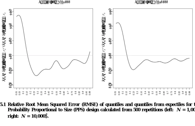
ˆ MSE ˆ MSE M R R Q Q   Dwellings 0.1 2.57 2.76 1.07 0.25 1.77 1.97 1.11 0.5 2.45 2.35 0.96 0.75 3.15 2.91 0.92 0.9 4.20 3.43 0.82 Villages 0.1 5.52 6.65 1.21 0.25 11.41 10.31 0.90 0.5 12.29 11.69 0.95 0.75 16.24 15.41 0.95 0.9 13.31 18.34 1.38

To obtain more insight we run a simulation scenario which involves a larger sample size of n = 100 selected from populations of sizes N = 1,000 and N = 10,000. We draw Y and X from a bivariate log standard normal distribution with  = 0 and  = 1. The variables Y and X are drawn such that the correlation between the variables is equal to 0.9. We again calculate the root mean squared error for a range of  values and show the relative efficiency of the expectile based approach in Figure 5.1. For better visual presentation we show a smoothed version of the relative efficiency. We notice a reduction in the root mean squared error for both cases N = 1,000 and N = 10,000. We may conclude that the expectiles can easily be fitted in unequal probability sampling and the relation between expectiles and the distribution function can be used numerically to calculate quantiles with increased efficiency. This efficiency gain holds for upper quantiles only, that is for  bounded away from zero. Note however that the sampling scheme is such that large values of Y are sampled with higher probability, reflecting that the sampling scheme aims to get more reliable estimates for the right hand side of the distribution function, i.e., for large quantiles. If we are

(9)

interested in small quantiles we should use a different samling scheme by giving individuals with small values of Y an increased inclusion probability. In this case the behavior shown in Figure 5.1 would be mirrored with respect to .

Figure 5.1 Relative Root Mean Squared Error (RMSE) of quantiles and quantiles from expectiles for the Probability Proportional to Size (PPS) design calculated from 500 repetitions (left: N = 1,000, right: N = 10,000 .

6 Discussion

In Section 4 we extended the toolbox of expectiles to the estimation of distribution functions in the framework of unequal probability sampling. We defined expectiles for unequal probability samples. When comparing quantiles based on ˆF_R with quantiles based on the expectile based estimator ˆ ,F_RM we observed that the proposed estimator performs well in comparison to existing methods. The calculation of empirical expectiles is implemented in the open source software R (see R Core Team 2014) and can be found in the R-package expectreg by Sobotka, Schnabel, and Schulze Waltrup (2013). The calculation of the expectile based distribution function estimator ˆM

N

F is also part of the R-package expectreg. The calculation of ˆF_RM is, however, more demanding as the calculation of ˆF_R because it involves three steps: First, we calculate the weighted expectiles as described in Section 3; second, we estimate ˆ ,N

R

F and in a third step, we derive ˆM

R

F from ˆF_RN (see Section 4). In the Log-Normal-Simulation it takes about 2-3 seconds for N = 1,000 to calculate ˆM

R

F whereas the computational effort of ˆF_R is barely noticeable.

Acknowledgements

Both authors acknowledge financial support provided by the Deutsche Forschungsgemeinschaft DFG (KA 1188/7-1).

Smooth fit for N = 1,000 Smooth fit for N = 10,000

RMSE Q ua nt il es from / RMSE Qu an ti les fr om 0. 90 0 .9 5 1 .00 1 .0 5 1 .1 0 1 .1 5 RMSE Q ua nt il es from / RMSE Qu an ti les fr om 0. 90 0 .9 5 1 .00 1 .0 5 1 .1 0 1 .1 5 α α

(10)

References

Aigner, D.J., Amemiya, T. and Poirier, D.J. (1976). On the estimation of production frontiers: Maximum likelihood estimation of the parameters of a discontinuous density function. International Economic Review, 17(2), 377-396.

Chambers, R.L., and Dunstan, R. (1986). Estimating distribution functions from survey data. Biometrika, 73(3), 597-604.

Chen, Q., Elliott, M.R. and Little, R.J.A. (2010). Bayesian penalized spline model-based inference for finite population proportion in unequal probability sampling. Survey Methodology, 36, 1, 23-34.

Chen, Q., Elliott, M.R. and Little, R.J.A. (2012). Bayesian inference for finite population quantiles from unequal probability samples. Survey Methodology, 38, 2, 203-214.

De Rossi, G., and Harvey, A. (2009). Quantiles, expectiles and splines. Nonparametric and robust methods in econometrics. Journal of Econometrics, 152(2), 179-185.

Guo, M., and Härdle, W. (2013). Simultaneous confidence bands for expectile functions. AStA - Advances in Statistical Analysis, 96(4), 517-541.

Hajek, J. (1971). Comment on “An essay on the logical foundations of survey sampling, part one”. The Foundations of Survey Sampling, 236.

Isaki, C.T., and Fuller, W.A. (1982). Survey design under the regression superpopulation model. Journal of the American Statistical Association, 77, 89-96.

Jones, M. (1992). Estimating densities, quantiles, quantile densities and density quantiles. Annals of the Institute of Statistical Mathematics, 44(4), 721-727.

Kish, L. (1965). Survey Sampling. New York: John Wiley & Sons, Inc.

Kneib, T. (2013). Beyond mean regression (with discussion and rejoinder). Statistical Modelling, 13(4), 275-385.

Koenker, R. (2005). Quantile Regression, Econometric Society Monographs. Cambridge: Cambridge University Press.

Kuk, A.Y.C. (1988). Estimation of distribution functions and medians under sampling with unequal probabilities. Biometrika, 75(1), 97-103.

Lahiri, D.B. (1951). A method of sample selection providing unbiased ratio estimates. Bulletin of the International Statistical Institute, (33), 133-140.

Midzuno, H. (1952). On the sampling system with probability proportional to sum of size. Annals of the Institute of Statistical Mathematics, 3, 99-107.

Murthy, M.N. (1967). Sampling Theory and Methods. Calcutta: Statistical Publishing Society.

Newey, W.K., and Powell, J.L. (1987). Asymmetric least squares estimation and testing. Econometrica, 55(4), 819-847.

(11)

Pratesi, M., Ranalli, M. and Salvati, N. (2009). Nonparametric M-quantile regression using penalised splines. Journal of Nonparametric Statistics, 21(3), 287-304.

R Core Team (2014). R: A Language and Environment for Statistical Computing. Vienna, Austria: R Foundation for Statistical Computing.

Rao, J., and Wu, C. (2009). Empirical likelihood methods. Handbook of Statistics, 29B, 189-207.

Rao, J.N.K., Kovar, J.G. and Mantel, H.J. (1990). On estimating distribution functions and quantiles from survey data using auxiliary information. Biometrika, 77(2), 365-375.

Schnabel, S.K., and Eilers, P.H. (2009). Optimal expectile smoothing. Computational Statistics & Data Analysis, 53(12), 4168-4177.

Schulze Waltrup, L., Sobotka, F., Kneib, T. and Kauermann, G. (2014). Expectile and quantile regression - David and Goliath? Statistical Modelling, 15, 433-456.

Sobotka, F., and Kneib, T. (2012). Geoadditive expectile regression. Computational Statistics & Data Analysis, 56(4), 755-767.

Sobotka, F., Schnabel, S. and Schulze Waltrup, L. (2013). Expectreg: Expectile and Quantile Regression. With contributions from P. Eilers, T. Kneib and G. Kauermann, R package version 0.38.

Tillé, Y., and Matei, A. (2015). Sampling: Survey Sampling. R package, version 2.7. https://cran.r-project.org/web/packages/sampling/index.html.

Yao, Q., and Tong, H. (1996). Asymmetric least squares regression estimation: A nonparametric approach. Journal of Nonparametric Statistics, 6(2-3), 273-292.