Multiagent planning with Bayesian nonparametric asymptotics

Multiagent Planning with Bayesian

Nonparametric

Asymptotics

by

Trevor D. J. Campbell

Submitted to the Department of Aeronautics and Astronautics

in partial fulfillment of the requirements for the degree of

Master of Science in Aeronautics and Astronautics

at the

MASSACHUSETTS INSTITUTE OF TECHNOLOGY

August 2013

©

Massachusetts Institute of Technology 2013. All

A uthor ...

...

Dep

n ent of Aeronautics

Certified by ...

...

rights reserved.

and Astronautics

August 22, 2013

Jonathan P. How

Richard C. Maclaurin Professor of Aeronautics and Astronautics

Thesis Supervisor

/

Accepted by...

rofessor Eytan H. Modiano

Professor of eronautics and Astronautics

Chair, Graduate Program Committee

MASSACHUSETTS IENIfE OF TECHNOLOGY

NOV

12

2013

Multiagent Planning with Bayesian Nonparametric

Asymptotics

by

Trevor D. J. Campbell

Submitted to the Department of Aeronautics and Astronautics on August 22, 2013, in partial fulfillment of the

requirements for the degree of

Master of Science in Aeronautics and Astronautics

Abstract

Autonomous multiagent systems are beginning to see use in complex, changing en-vironments that cannot be completely specified a priori. In order to be adaptive to these environments and avoid the fragility associated with making too many a priori assumptions, autonomous systems must incorporate some form of learning. How-ever, learning techniques themselves often require structural assumptions to be made about the environment in which a system acts. Bayesian nonparametrics, on the other hand, possess structural flexibility beyond the capabilities of past parametric tech-niques commonly used in planning systems. This extra flexibility comes at the cost of increased computational cost, which has prevented the widespread use of Bayesian nonparametrics in realtime autonomous planning systems.

This thesis provides a suite of algorithms for tractable, realtime, multiagent plan-ning under uncertainty using Bayesian nonparametrics. The first contribution is a multiagent task allocation framework for tasks specified as Markov decision processes. This framework extends past work in multiagent allocation under uncertainty by al-lowing exact distribution propagation instead of sampling, and provides an analytic solution time/quality tradeoff for system designers. The second contribution is the Dynamic Means algorithm, a novel clustering method based upon Bayesian nonpara-metrics for realtime, lifelong learning on batch-sequential data containing temporally evolving clusters. The relationship with previous clustering models yields a modelling scheme that is as fast as typical classical clustering approaches while possessing the flexibility and representational power of Bayesian nonparametrics. The final contri-bution is Simultaneous Clustering on Representation Expansion (SCORE), which is a tractable model-based reinforcement learning algorithm for multimodel planning problems, and serves as a link between the aforementioned task allocation framework and the Dynamic Means algorithm.

Thesis Supervisor: Jonathan P. How

Acknowledgments

There are a number of people who have my utmost appreciation for helping me along my travels here at MIT. First and foremost, my advisor Jon - it has been, and will continue to be, a pleasure exploring and developing the world of autonomous planning with you. Your supervision has been crucial in shaping my research interests, how I

approach problems, and how I communicate my findings to the academic world. In no uncertain terms do I owe my success in my endeavours to my friends and family. Mom, Dad, Emily - thank you for keeping me sane, giving me a brief respite from the fast-paced world of research from time to time, and celebrating with me when I made breakthroughs. To my group of awesome friends from the University of Toronto - Sean, Rick, Manan, Jamie, Konstantine, Adam, Sanae, Catherine, Amy, Angela, and countless more - thanks for sticking with me through thick and thin. To my new friends here at MIT - Sam, Luke, Buddy, Ian, Dan, Andrew, Kemal, Bobby, Chris, Jack, Rob, Kane, Miao, Andrew, Nikhil, Vyas, and everyone else - thanks for making me feel right at home here in Boston. To Brendan, I've had the time of my life being a student of yours - you've opened my mind to a completely new world of improvisation, voicings, and keyboard geometry that, until meeting you, I had no idea existed.

Last, but most certainly not least, I thank my wonderful girlfriend Maria. Your love and support have been the foundation upon which I have stood, and your per-severence in your own academics is an inspiration to me.

This work was supported by ONR MURI Grant N000141110688, and a Natural Sciences and Engineering Research Council of Canada PGS-M grant.

For fifteen days I struggled to prove that no functions analogous to those I have since called Fuchsian functions could exist. I was then very ignorant; every day I sat down at

my work table where I spent an hour or two, tried a great number of combinations and arrived at no result. One evening, contrary to my custom, I took black coffee. I could not

go to sleep; ideas swarmed up in clouds, and I sensed them clashing until, to put it so, a pair would hook together to form a stable combination. By morning I had established the existence of a class of Fuchsian functions, those derived from the hypergeometric series. I

had only to write up the results, which took but a few hours.

Contents

1 Introduction

1.1 Overview. . . . .

1.2 Literature Review and Analysis . . . . 1.3 Thesis Contributions and Organization

2 Background

2.1 Overview. . . . . 2.2 Bayesian Nonparametrics . . . . 2.3 Markov Decision Processes . . . . 2.4 Multiagent Task Allocation . . . .

3 Multiagent Allocation of Markov Decision Process Tasks 3.1 Overview ... ...

3.2 Introduction . . . . 3.3 Problem Statement . . . . 3.4 MDP Task Model . . . . 3.5 Task Sequence Evaluation . . . .

3.6 Computing Starting State/Time Distributions . . . .

3.7 Algorithm and Complexity Analysis . . . .

3.8 Example: Target Identification . . . .

3.9 Sum m ary . . . . 4 The Dynamic Means Algorithm

4.1 O verview . . . . 4.2 Introduction . . . . 4.3 Asymptotic Analysis of the DDP Mixture . . . .

4.4 The Dynamic Means Algorithm . . . . 4.5 A pplications . . . . 9 9 11 16 19 19 19 33 38 41 41 42 44 45 46 48 51 52 56 57 57 58 60 64 70

. . . .

. . . .

. . . .

4.6 Summary ... ... 74

5 SCORE: Simultaneous Clustering on Representation Expansion 77

5.1 O verview . . . . 77 5.2 Introduction ... ... 78 5.3 Simultaneous Clustering On Representation Expansion (SCORE) . . 80 5.4 Experimental Results . . . . 85 5.5 Sum m ary . . . . 87 5.6 A ppendix . . . . 88

6 Conclusions 91

6.1 Summary and Contributions . . . . 91 6.2 Future W ork . . . . 92

Chapter 1

Introduction

1.1

Overview

Autonomous multiagent systems are becoming increasingly prevalent in situations in-volving complex, changing environments that cannot be completely specified a priori [1-5]. In such situations, the system must coordinate and make decisions based upon information gathered from the environment in which it acts. There are a number of ways to take observed data into account when planning; one of the most popu-lar techniques is a model-based approach, where observations are used to update a compact, approximate representation (a model) of the environment, and decisions are made with respect to that model. Having an accurate model is often paramount to the success of the autonomous system; however, in realistic missions, an accurate model generally cannot be obtained with certainty. The observations made by the system are often noisy, incomplete, and local, leading to uncertainty in which model best captures the relevant aspects of the environment.

A principled approach of dealing with this uncertainty is to use a probabilistic model of the environment. Such techniques involve specifying an initial model, which is then updated using Bayesian posterior inference as observations are made [6-8]. This initial model has, in the vast majority of probabilistic planning literature, fallen into the class of parametric probabilistic models (e.g. the beta-Bernoulli model [9]). The use of such parametric models requires the system designer to take a certain leap

of faith; parametric models assume the structure of the model, or its number of con-stituent components, is well-known and fixed. Of course, both of these assumptions are routinely violated by real-world planning missions; the model structure is rarely known a priori, and even more rarely is it constant throughout the duration of the mission.

Bayesian nonparametric models (BNPs), on the other hand, are a class of proba-bilistic models in which the number of parameters is mutable, and may be modified during posterior inference [10-15]. BNPs have a flexible structure and, therefore, are particularly useful in situations where it is not clear what the model structure should be a priori. The designer is thus free from specifying the model structure, instead allowing the system to discover it through interactions with its environment. However, the enhanced flexibility of Bayesian nonparametrics with respect to their parametric counterparts does not come without a cost. Current inference techniques, such as Gibbs sampling [16], variational inference [17], stochastic variational inference

[18], and particle learning [19], are not computationally competitive with parametric

inference techniques.

This problem of computational tractability is not unique to the learning compo-nent of a model-based autonomous system; past approaches to multiagent planning under uncertainty suffer from similar pitfalls. Markov decision processes (MDPs) are a natural framework for describing sequential decision-making problems, can capture rich forms of uncertainty in the evolution of the surrounding environment, and have been used in a wide variety of applications [20]. However, they suffer from the "curse of dimensionality": the difficulty of solving the planning problem scales exponentially with the number of agents in the system. Recent approaches have mitigated this to an extent, but are still computationally expensive and sacrifice explicit, guaranteed coordination [21]. Multiagent task allocation approaches, on the other hand, have a computational cost that scales polynomially in the number of agents, and guarantee explicit coordination; however, to date, all such methods that account for uncertainty do not perform model learning based on observations, and require computationally expensive sampling procedures to evaluate the performance of candidate allocations

[22]. The issues of computational cost (both incurred by the learning and plan-ning procedures) are particularly relevant when considering the computational power available in current embedded systems, such as those found in many autonomous multiagent systems.

Thus, the goal of this thesis is the development of a Bayesian nonparametric model-based multiagent planning system, with a focus on the tractable incorporation of uncertainty at both the planning and learning stages.

1.2

Literature Review and Analysis

Multiagent Task Allocation Task allocation algorithms generally solve the prob-lem of deciding, given a list of tasks to do and available resources, an assignment of resources to tasks that maximizes some notion of overall system performance [23]. The problem statement most commonly used is that of a general mixed-integer, nonlinear optimization program. As this mathematical program is intractable to solve exactly, solution techniques generally involve heuristics (e.g. sequential greedy allocation). Re-cent advances in this literature have provided polynomial-time, asynchronous, decen-tralized auctions with guaranteed convergence [24-28], but such advances are designed to provide assignments when task models have a constant, deterministic state (e.g. visiting a set of waypoints). These greedy assignment algorithms have, however, been extended to include the effects of stochastic parameters on the overall task assignment process, and have considered robust, chance-constrained, and expected performance metrics [22, 29]. The most successful of these were the chance-constrained approaches; however, they rely on sampling a set of particles from the distributions of stochastic parameters and making informed decisions based on those particles, with no notion of solution quality vs. the number of propagated samples. Further, these approaches do not incorporate learning to improve the stochastic models over time. Conversely, there are approaches which do incorporate learning (e.g. the Intelligent Cooperative Control Architecture (iCCA) [30, 31]) to reduce model uncertainty, but plan using the expected model and do not actually account for the uncertainty in the model during

the allocation procedure itself. Thus, while scalable coordination under uncertainty has been studied within this framework, the areas of concurrent learning and alloca-tion under uncertainty, and exact evaluaalloca-tion of assignment score under uncertainty remain un-addressed.

Markov Decision Processes In the framework of Markov decision processes, ex-plicit and guaranteed multiagent coordination for general problems is well known to exhibit exponential computational scaling with respect to the number of agents in the team [21]. On the other hand, a number of previous studies have explored the benefits of decomposing MDPs into smaller weakly coupled [32] concurrent processes, solving each individually, and merging the solutions to form a solution of the larger problem [33, 34]. Building on that work, several researchers have considered problems where shared resources must be allocated amongst the concurrent MDPs [32, 35]; gen-erally, in such problems, the allocation of resources amongst the MDPs determines which actions are available in each MDP, or the transition probabilities in each MDP. Some approaches involve solving resource allocation or coordination problems by mod-elling them within the MDP itself [36, 37]. Assignment based decompositions have also been studied [38], where cooperation between agents is achieved via coordinated reinforcement learning [39]. However, none of these approaches have considered the impact of previous tasks on future tasks. This is of importance in multiagent multi-assignment planning problems; for instance, if an agent is assigned a task involving a high amount of uncertainty, that uncertainty should be properly accounted for in all of its subsequent tasks (whose starting conditions depend on the final state of the uncertain task). This allows the team to hedge against the risk associated with the uncertain task, and allocate the subsequent tasks accordingly. Past work has focused primarily on parallel, infinite-horizon tasks [32, 35], and have not encountered the cascading uncertainty that is characteristic of sequential bundles of uncertain tasks.

Bayesian Nonparametrics - Learning Several authors have explored BNP

BNPs have been used for speaker diarization [14], for document classification [11], for classifying life history data [46], and for classifying underwater habitats [47]. Many Bayesian nonparametric models exist, such as the Dirichlet process and its hierar-chical variant [10, 11], the beta process and its hierarhierar-chical variant [13], and the dependent Dirichlet process [12, 48]. The Dirichlet and dependent Dirichlet processes are the primary BNPs used in this thesis; the reader is encouraged to consult the references for more complete discussions of the other existing models.

The Dirichlet process mixture model (DPMM) is a powerful tool for clustering data that enables the inference of an unbounded number of mixture components, and has been widely studied in the machine learning and statistics communities [17, 19, 49, 50]. Despite its flexibility, it assumes the observations are exchangeable, and therefore that the data points have no inherent ordering that influences their labeling. This assump-tion is invalid for modeling temporally/spatially evolving phenomena, in which the order of the data points plays a principal role in creating meaningful clusters. The de-pendent Dirichlet process (DDP), originally formulated by MacEachern [48], provides a prior over such evolving mixture models, and is a promising tool for incrementally monitoring the dynamic evolution of the cluster structure within a dataset. More recently, a construction of the DDP built upon completely random measures [12] led to the development of the dependent Dirichlet process Mixture model (DDPMM) and a corresponding approximate posterior inference Gibbs sampling algorithm. This model generalizes the DPMM by including birth, death and transition processes for the clusters in the model.

While Bayesian nonparametrics are powerful in their capability to capture com-plex structures in data without requiring explicit model selection, they suffer some practical shortcomings. Inference techniques for BNPs typically fall into two classes: sampling methods (e.g. Gibbs sampling [50] or particle learning [19, 51]) and optimiza-tion methods (e.g. variaoptimiza-tional inference [17] or stochastic variaoptimiza-tional inference [18]). Current methods based on sampling do not scale well with the size of the dataset [52]. Most optimization methods require analytic derivatives and the selection of an upper bound on the number of clusters a priori, where the computational complexity

in-creases with that upper bound [17, 18]. State-of-the-art techniques in both classes are not ideal for use in contexts where performing inference quickly and reliably on large volumes of streaming data is crucial for timely decision-making, such as autonomous robotic systems [53-55]. On the other hand, many classical clustering methods

[56-58] scale well with the size of the dataset and are easy to implement, and advances

have recently been made to capture the flexibility of Bayesian nonparametrics in such approaches [57-60]. There are also a number of sequential Monte-Carlo methods that have capabilities similar to the DDP mixture model [61, 62] (of which particle learn-ing may be seen as a generalization). However, as of yet, there is no algorithm that captures dynamic cluster structure with the same representational power as the DDP mixture model while having the low computational workload of classical clustering algorithms.

Bayesian Nonparametrics - Planning Within the context of planning, BNPs are just beginning to make a substantial impact. The robotics community has per-haps made the most use of BNPs so far; however, the attention here has been limited primarily to Gaussian processes (GPs). GP-based models have been used for regres-sion and classification [15], for Kalman filtering [63], and for multistep lookahead predictions [64]. Several authors have also used GPs for planning in the framework of dynamic programming and reinforcement learning [65, 66], and in motion planning in the presence of dynamic, uncertain obstacles [67]. The Dirichlet process (DP) has been combined with the GP to form the DPGP mixture model, which has seen use in target tracking [68]. Finally, hierarchical Dirichlet processes have seen use in various Markov systems, such as hidden Markov models [14] and partially observable Markov decision processes [69]. This lack of substantial BNP research in planning has been noted in previous studies [70].

Multiple Model-based Reinforcement Learning This thesis employs model-based reinforcement learning (RL) to capture systems that exhibit an underlying multiple-model (or multimodel) structure, i.e. those that can be described as a

col-lection of distinct models with some underlying mechanism for switching between them. Generally speaking, the model-based RL paradigm involves building an accu-rate model of a MDP from observed interactions [71, 72]. There is a vast body of prior literature on model-based reinforcement learning methods, such as classical methods (e.g. Dyna [71, 73, 74]), Bayesian methods (e.g. BOSS [75], BEETLE [76]), methods with statistical error bounds (e.g. R-Max [77], KWIK [78]), among others. However, these techniques do not incorporate the aforementioned multimodel structure, result-ing in a learned model that is the average over the set of underlyresult-ing models. Early work on controlling systems with multiple models that does take advantage of the structure, such as MOSAIC [79] and MPFIM [80], used a softmax mixture of control experts where weights are determined by predictive likelihood. Multiple model-based reinforcement learning (MMRL) [81], built upon these methods, involves using a mixture of experts for the model representation, where the weighted experts are used for updating value functions, models, and deciding which action to take. MOSAIC-MR [82] extends MMOSAIC-MRL and MOSAIC to the case where changes in the reward function are unobservable, and does not pair controllers a priori with fixed predictors of dynamics and reward. One major drawback of approaches such as MOSAIC-MR is that the number of models is fixed and known a priori, as is the chosen representation; this limits the capability of such approaches to handle situations where the number of models is unknown a priori, in addition to their individual complexity. Outside of the domain of reinforcement learning, a number of Bayesian nonparametric methods exist that learn an unknown number of underlying models within a single system. For example, the sticky HDP-SLDS-HMM and HDP-AR-HMM [83] learn a set of linear or autoregressive dynamical systems, where the switching between the models is con-trolled by a hidden Markov model with an unknown number of states. However, the structure of each underlying model is fixed and does not adapt to better capture the data. The DPGP [68] is a good example of a BNP that learns an underlying multiple model structure; the number of models is unknown, and each Gaussian process (GP) model adapts to fit the data assigned to it. However, using the original DPGP (and indeed, most Bayesian nonparametric inference techniques [17-19]) in an RL setting

is impractical due to the complexity of inference.

1.3

Thesis Contributions and Organization

The rest of this thesis proceeds as follows. Chapter 2 provides a technical background in Bayesian nonparametric modelling, Markov decision processes, and multiagent task allocation. Chapters 3, 4, and 5 highlight the three major contributions of this thesis:

9 Chapter 3 presents the development of a multiagent task allocation framework

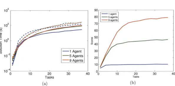
for tasks specified as Markov decision processes. This framework extends past work in multiagent allocation under uncertainty by incorporating the generality of Markov decision processes, allows exact distribution propagation instead of sampling, and provides an analytic solution time/quality tradeoff for system designers. Empirical results corroborate the theoretical results, demonstrating that this method remains tractable in the presence of a large number of agents and uncertain tasks. The discussion in this chapter makes the assumption that all system models are well-known.

9 Chapter 4 introduces the tool that will serve to relax the assumption that the

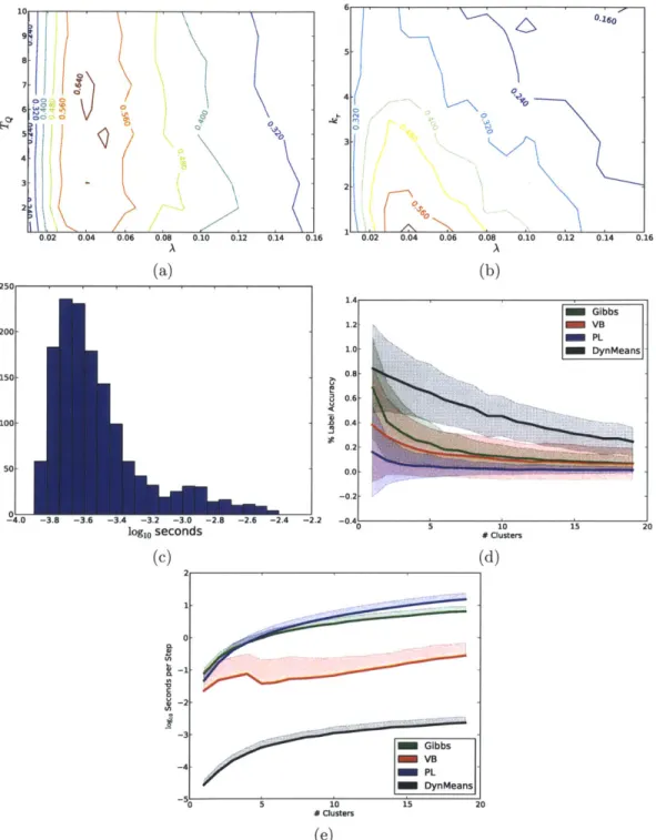
system models are well known: the Dynamic Means algorithm, a novel clustering method based upon Bayesian nonparametrics for real-time, lifelong learning on batch-sequential data containing temporally evolving clusters. This algorithm is developed by analyzing the low-variance asymptotics of the dependent Dirichlet process mixture model, and is guaranteed to converge in a finite number of iterations to a local optimum in a k-means-like cost function. Empirical results demonstrate that the Dynamic Means algorithm is faster than typical classical hard and probabilistic clustering approaches, while possessing the flexibility and representational power of Bayesian nonparametrics.

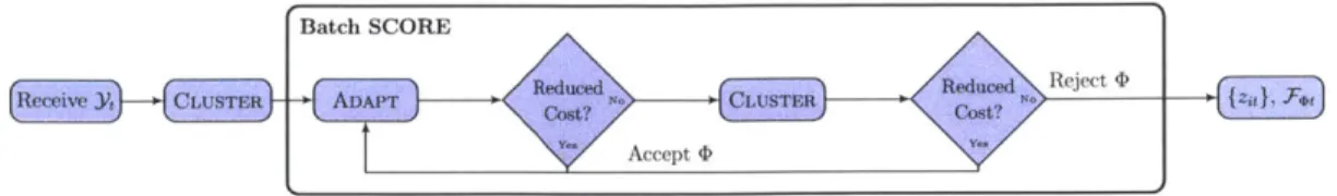
* Chapter 5 discusses a reinforcement learning framework, the Simultaneous Clus-tering on Representation Expansion (SCORE) algorithm, that links the con-cepts in Chapters 3 and 4. By combining the strengths of representation

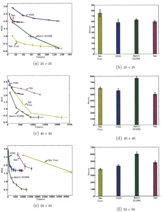
expan-sion and hard clustering, this algorithm provides a method for fast, model-based reinforcement learning when the planning problem is large and exhibits an un-derlying multiple-model structure. The algorithm is guaranteed to terminate in a finite number of iterations to a local optimum in a combined clustering-expansion cost function. Empirical results on a simulated domain demonstrate that this method remains tractable for large state-spaces and outperforms con-temporary techniques in terms of both the sample and time complexity of learn-ing.

The three aforementioned contributions together form a full toolset for combined planning and learning, which operates in real-time and has the flexibility of Bayesian

nonparametrics.

Finally, Chapter 6 concludes the thesis and provides future directions for further investigation.

Chapter 2

Background

2.1

Overview

This chapter provides a comprehensive review of the background material required to understand this thesis. It covers the basics of Bayesian nonparametric modeling and inference (and in particular, the Dirichlet and dependent Dirichlet processes), Markov decision processes, and multiagent task allocation.

2.2

Bayesian Nonparametrics

Bayesian modelling and inference generally involves using measurements to improve a probabilistic model of an observed phenomena. The two major components of a Bayesian probabilistic model are the likelihood and the prior distributions: The likelihood p(yl0) is a distribution that represents the probability of the observed data y given a set of parameters 0, while the prior p(O) represents the probability distribution over those parameters (sometimes referred to as latent variables) before any observations are made. As measurements become available, the prior is combined with the likelihood of those measurements using Bayes' rule, resulting in a posterior distribution p(O1y) over the parameters 0:

P(Y)

=

Y

O)

(2.1)

Where the posterior may be thought of as an updated distribution over 0 that takes into account all information contained in the observations y.

If the posterior p(Oly) is of the same family of distributions as the prior p(0), when

using a particular likelihood p(y

10),

the prior is said to be conjugate to that likelihood. For example, if yj1 - .(0, a2_{), then 0}

~ M(pt, F2) is a conjugate prior that results

in the posterior distribution Oly M ( P 4

+

I ) , where fi(a, b) is a normal

distribution with mean a and variance b. In other words, a normal prior is conjugate to a normal likelihood. The use of conjugate priors leads to an ability to perform closed-form, exact posterior inference, rather than relying on approximate methods; in this case, the hyperparameters (parameters of the prior p(O)), p and T, can be

updated analytically to M' = P + Y and T' 1 1 This capability becomes

T2 U2

very important when dealing with complex Bayesian models, where the closed-form conjugate updates constitute part of a larger inference algorithm [16].

Typically, a Bayesian model is specified in terms of a generative model, which is a conceptual process by which the observations are assumed to be created. The generative model defines the likelihood(s) and prior(s) for use in inference. As a brief illustrative example, say there is a database of N images yi of K objects, where the object in each image is unlabelled. In order to label the images in terms of the object they contain, the images must be grouped into K bins, one for each object. An appropriate generative model for this situation might be as follows:

1. For each bin k 1, ... , K, sample a set of parameters Ok - H

2. For each i = 1, ... , N, roll a weighted K-sided die and observe the outcome zi

3. For each i = 1, . ., N, sample the image y _~ A'(0zi, U2

)

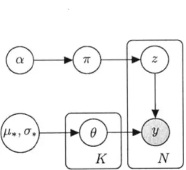
If written mathematically, this can be expressed as:

7rla ~ Dir(ai, .. , aK)

ziJ7 ~ Categorical(7r), i 1,..., N

(2.2)

Oy ,

) k=

,...,

K N

Figure 2-1: Dirichlet mixture graphical model

where the latent variables of the generative model are as follows:

0 7r = (7r1, . . -rK K,

Zk

7rk = 1 are a set of positive weights that sum to 1 (the

probabilities of the weighted K-sided die),

0 {zi}'i 1, zi E {1,. . ., K} are the bin index labels for each image,

0 0 = (01,... , 6K) are the parameters that govern the appearance of each object. The hyperparameters of the prior are a:, .. ., aK > 0, and represent imaginary counts

of rolls from the weighted K-sided die before the experiment begins. For example, setting a1 = 100, and ak = 0.1, k = 2, ... , K creates a high prior certainty on side 1 of the die being heavily weighted (as if a die were rolled 100 times and landed on the 1 side every time), while setting ak = 100, k = 1, ... , K creates a high prior certainty that the die is fair (as if a die were rolled 100K times, and landed on each side 100 times). The ak may be selected by hand, in which case a larger set of a:,.. . , aK > 0

yields a stronger prior that requires more data to overcome, and vice versa for smaller

aQ,...,aK >

0-This particular generative model has a name: the Dirichlet mixture model [84]. Of course, this is not how the images were actually created; it is simply a conceptual process in order to derive appropriate likelihood and prior distributions over the data and latent variables. Here, the prior distributions are the Dirichlet-Categorical distribution over 7r and zi, and the multivariate Gaussian distribution over 0; and the likelihood is the Gaussian distribution over yi. As measurements become available, the estimates of 7r and 0 can be improved via Bayesian inference.

the number of parameters or latent variables in the model are fixed a priori (in this case, the K mixing probabilities and parameters), and are often chosen through expert judgment. Bayesian nonparametric models, in contrast, do not require the expert specification of the number of parameters; instead, the number of parameters in such models is infinite, while a finite quantity of observed data is assumed to be generated using only a finite subset of those parameters. This allows Bayesian inference techniques to learn the number of latent variables in a model, in addition to their values.

Table 2.1 presents a list of standard and recently developed Bayesian nonparamet-ric models [85]. The Gaussian process (GP) is perhaps the most well known example of a BNP in the planning community, and is typically used as a model for continuous functions. GP-based models have been used for regression and classification [15], for Kalman filtering [63], and for multistep lookahead predictions [64]. Several authors have also used GPs for planning in the framework of dynamic programming and rein-forcement learning [65, 66], in motion planning in the presence of dynamic, uncertain obstacles [67], and in predicting pedestrian motion [86]. The Dirichlet process (DP) and beta process (BP), on the other hand, are well-known nonparametric models in the machine learning community [10, 14, 17, 85], but have seen very few applications in planning and control, despite their ability to robustly capture the complexity of a system solely from observations [68, 87]. The DP and BP also serve as building blocks for other Bayesian nonparametric priors, such as the dependent Dirichlet pro-cess (DDP) [12], the hierarchical Dirichlet propro-cess (HDP) [11], and the hierarchical Beta process (HBP) [13].

This thesis is focused on the applications and advantages of the DDP and models based thereupon in planning systems. As such, the DP and DDP will be explained in detail in the following; citations for the other common Bayesian nonparametrics may be found in the list of references.

Table 2.1: Typical BNPs with applications [85]

Model Typical Application

GP Learning continuous functions

DP Data clustering, unknown

#

of static clusters BP Latent feature models, unknown

#

of features DDP Data clustering, unknown

#

of dynamic clusters HDP Topic modeling, unknown # topics, words

HBP Shared latent feature models, unknown

#

features

2.2.1

The Dirichlet Process

Recall that the Dirichlet distribution in the earlier mixture model example (2.2) is a prior over unfair K-sided dice, and is used in mixture models with K components. One might naturally wonder whether the mixture model can be relaxed, such that K can be learned from the data itself without expert specification. As mentioned in the previous section, this might be accomplished by assuming that K -+ o (in a sense), and then taking advantage of the fact that a finite quantity of data must have been generated by a finite number of components.

Proceeding based on this notion, let the k- dimensional unit simplex be defined as the set of vectors 7r = (71, ... , 7rK) E RK such that EZ 1ri = 1, and 7ri ;> 0 for all i.

Then, the Dirichlet distribution is a probability distribution over this K-dimensional unit simplex whose density is given by:

p(7r) =() ,(2.3)

where F(-) is the Gamma function, and oz (ai, ... , QaK) is a parameter vector. If one sets (aa, ... , cK) = , ..., for some a > 0, taking the limit as K -+ oc creates a

K K

Dirichlet distribution whose draws contain an infinite number of components that sum to 1. This is the intuitive underpinning of the Dirichlet process (DP). The definition of a Dirichlet process is as follows (developed formally in [44]):

Definition 2.2.1 [44] Let H be a probability measure on a space X, and let a > 0 be

a real number. Then G ~ DP(a, H) is a probability measure drawn from a Dirichlet process if for any finite partition {B1, ..., BN} of X (i.e. Bi

flB

= 0 for all i -p

j

N

and

U

Bi = X),

i=1

(G(B

1

),

...,

G(BN))IH, a

~

Dir(aH(B1),

..., aH(BN))-

(2.4)

This definition illustrates the fundamental difference between the conceptual "infi-nite Dirichlet distribution" described earlier and a Dirichlet process: samples from the former are oo-dimensional vectors, while samples from the latter are probability measures on some space X. Further, it can be shown that E [G(B)] = H(B), and that V [G(B)] = H(B)(1 - H(B))/(a + 1) for any B C X [10]. This provides a sense of how H and a influence G: H, called the base measure, is essentially the mean of G; and a, called the concentration parameter, controls its variance. Occasionally, one may use the notation G ~ DP(p), where p is a measure on X that does not necessarily sum to 1. In this case, it is understood that a =

fx

dy, H = t/a.

The definition of the Dirichlet process is admittedly rather hard to draw any useful conclusion from at first glance. However, it can be shown that G is discrete with probability 1, and has the following form [88]:

o

G = Zrioi, (2.5)

i=1

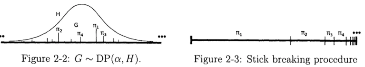
where the weights ri satisfy E ri = 1, 6, is an atom at x E X, and Oi ~ H are the locations of the atoms. A representation of G is shown in Figure 2-2. This provides a mental picture of what a DP is: it can be thought of as a distribution, which, when sampled, yields another probability distribution G having a countably infinite number of atoms on a space X. Each atom has independent and identically distributed (i.i.d.) location within X with distribution H (with a slight abuse of notation , we use H to both refer to the measure and its related continuous distribution), where the weights

7ri on the atoms can be thought of as being drawn from an infinite dimensional

Dirichlet distribution.

In order to sample G from a DP, the stick breaking construction is typically

pro-H

G T1

12 T14 113 TE1 12 1131 4

0-'"Ii iI I

I

fill'

Figure 2-2: G ~ DP(a, H). Figure 2-3: Stick breaking procedure vides an iterative procedure for sampling the weights of (2.5), given by:

i-1

7ri =

#i

H(1 #) (2.6)

j=1

where

/3

~ Beta(1, a) are sampled from the beta distribution. As shown in Fig.

2-3, this corresponds to taking a stick of unit length, repeatedly breaking off beta

distributed pieces, and assigning them to locations

0,

in X. Thus, to sample a draw from a DP, we simply alternately sample 0% from H, and calculate the corresponding 7i

by sampling O3. Of course, there are theoretically an infinite number of (7ri,

O)

pairs, but the stick breaking process can be terminated to obtain an approximation after a finite number of steps by re-normalizing the weights to sum to 1, or by assigning whatever remaining probability mass there is to the last 0%.

Posterior inference for the Dirichlet process prior shares strong connections to posterior inference for the Dirichlet distribution. Consider once again the parametric mixture model in (2.2); it was not stated earlier, but the Dirichlet distribution is the conjugate prior of the categorical (or more generally, multinomial) likelihood. In other words, if one wishes to learn the outcome probabilities on a K-sided unfair die, one may observe N outcomes zi of the die, and then apply Bayes' rule:

7 ~ Dir(OZ1, ...., aK)

{zi} - Multinomial(7r) (2.7)

7rJ.{zi}

₁ ~ Dir(ai + ni,... , aK+ nK)

where nk = i =

k],

and the posterior 7rI{zi} I 1 is another Dirichlet distribution

due to conjugacy.

oo-dimensional Dirichlet distribution hints that the Dirichlet process is also conjugate to the categorical/multinomial likelihoods. Indeed this is the case; the posterior of a Dirichlet process after observing N samples

0,

drawn from G ~ DP is

G

DP(a,

H)

{ 1 ~ G _(2.8)

G1{ } 1~ DP

a,

a

H

1

a+N

a

+N

_

where the old base measure H is replaced by a weighted combination between H and the observed atoms o, with the weighting determined by a. However, as with the Dirichlet distribution, the Dirichlet process is most useful as a prior over mixture models where the

Oi

themselves are not measured directly, but rather some noisy measurements yi that depend on

0%.

Thus, while this description of the posterior Dirichlet process is illustrative mathematically, something more is required, practi-cally speaking.

Towards this goal, a probabilistic model which is closely related (this relation will be elucidated shortly) to the Dirichlet process is the Chinese Restaurant process (CRP) [101. This stochastic process models a sequence of data

Oi

as being generated sequentially, and upon generation of each data point, it is assigned a random label zi. Suppose a finite subset of such a sequence as been observed, and k unique labels have been assigned; then,

pAzn.+1=jilzi,...Z')=

_{a + n}

, Vj <k

(2.9)

p(zn+1 = k

+

llzi,..., zn)

a

+

n

where nr = 1 [zi =

j].

The name of the CRP comes from an analogy often used to describe it, which is illustrated in Fig. 2-4. If we consider a restaurant with an infinite line of tables, where customers enter and either sit at a previously selected table with probability proportional to the number of customers already sitting at that table, or start a new table with probability proportional to a, the table assignments are said

n+1

p(Zn+1=lla,Zi...n)c 5 p(zn+1=2Ia,zi...Oc 3 p(zn+1=3|a,zi)...O a

Figure 2-4: A pictorial representation of the CRP.

to be drawn from a Chinese Restaurant Process.

Perhaps the most useful fact about the CRP is that the labels zi are exchangeable:

Definition 2.2.2 A sequence of random variables z1, z2,... is exchangeable if for any

finite

collection zil, zi2, ... , ZiN7

p(zilzi2 , ..., iN)==P(zkz

1

Zk

2 ... zkN) (2.10)

for all permutations {ki, k2, ... , kN} of ii, i2,. - -,

iN}.-The fact that the observations zi in (2.9) are exchangeable is clear because the dis-tributions only depend on the number of times previous labels have been observed, and not their order. The reason why this is so important is due to de Finetti's the-orem [10]; informally, this thethe-orem states that if a sequence of random variables is exchangeable, then there exists an underlying distribution which explains the data as if it were sampled i.i.d. from that distribution. Using de Finetti's theorem, the CRP and the DP can be shown to be equivalent - As each sequential data point is observed, it is impossible to tell whether it was sampled i.i.d. from the distribution

G - _{DP(a, H) or whether it was generated from the sequential cluster assignment}

rules of the CRP.

Thus, approximate posterior inference for the DP can be conducted using the distributions provided by the CRP. This will be discussed further in the following. The reader is encouraged to consult [10] for further discussion of the Dirichlet process.

2.2.2

The Dependent Dirichlet Process

The major strength of the Dirichlet process as a prior over mixture models is that it infers K, the number of components in the model, directly from the data in a Bayesian framework. While this level of functionality is sufficient for a wide variety of applica-tions (from topic modeling [89] to trajectory pattern clustering [68]), in the context of planning it has a major weakness. The Dirichlet process is a static model that assumes that the data was generated from an unchanging set of mixture components. Autonomous planning systems often operate in dynamic environments where condi-tions are constantly changing, and even perhaps adapting to the system's behavior. Thus, it is important for a model to have the flexibility to deal with changing, novel, and disappearing characteristics in the environment. The assumption that mixture parameters are static is a hinderance to the DP's use in such environments. Further, this assumption has the unfortunate effect that all the data must be processed in

batch during inference, leading to ever-increasing computational costs as time goes

on and more data is collected.

The dependent Dirichlet process (DDP) [48] is a BNP model that extends the DP and remedies the aforementioned problems. The fundamental notion of the DDP is that it is essentially a Markov chain of DPs, where the transitions between DPs allows mixture components to change, disappear, or to be newly created. This gives the DDP additional flexibility over the DP that is required in many autonomous planning system environments. Further, the Markov property of the system allows inference to consider data in a batch-sequential framework, where only small subsets of the total dataset ever need to be stored or processed at once.

There are a number of equivalent definitions of the DDP, but perhaps the most illustrative one (and the one upon which a large portion of the present work is built) is based on Poisson processes [12]:

Definition 2.2.3 Let X be a measure space, and let

4

: X -+ [0, oo) be an integrable

intensity function on X, where T(B) = fB

4

is the mean measure for all measurable

such that the number of points in B C X, N(B) =

IFn BI

is a random number with a Poisson distribution N(B) ~ po('I(B)).

Suppose that a Poisson process is defined over some space X x [0, oo) (also known as a Gamma process or compound Poisson process). Then each atom i of the point process consists of a point Oi E X and a point 7Tr E R+ that may be thought of as a

ir'

weight on 0%. If the weights are then normalized, such that 7ri = ,the new point

zi

rr

process G with the normalized weights is a Dirichlet process G DP(oZ, H) with a = T (X x [0, oo)) and H is proportional to

4

with the part over the positive reals integrated out. This is referred to as a Poisson process construction of the Dirichlet process.

The reason why this construction is of particular importance is because a Poisson process can be probabilistically mutated in a number of ways such that the resulting point process is still a Poisson process. Thus, if a Dirichlet process is formulated in terms of its underlying Poisson process, such operations are performed on the underlying process, and then the weights are renormalized to be a Dirichlet process once again, one can think of the entire procedure simply as operations upon Dirichlet processes that preserve Dirichlet processes. The following operations preserve Poisson

processes [901:

Proposition 2.2.4 Superposition: Let P ~ UP(I),

Q

~ HP(Q) be Poisson pro-cesses. Then

P

U Q

~

HP(T + D).

Proposition 2.2.5 Subsampling: Let P ~ UP(I) be a Poisson process on X

with mean measure 4' and corresponding intensity V', let q : X -+ [0,1], and let bi ~ Be(q(0i)) be a Bernoulli trial for every 0, E P. Then

Q

= {0 E P : bi = 1} is a

Poisson process, where

Q

- UlP(4) and 1(B) = fB q.

Proposition 2.2.6 Transition: Let P ~ HP(P) be a Poisson process on X with

mean measure I and corresponding intensity

4.

Then suppose T : X x X -> R+,

where T(.0) is a probability distribution on X. For every 04 E P, let 0; ~ T(0{|0j). Then

Q

= {0} ~- H P(1) is a Poisson process with intensity $ fx T(0'j0)V'(0).

When the basic operations on Poisson processes are ignored and the operations are formulated entirely on Dirichlet processes, superposition is denoted U, subsampling with the function q is denoted Sq, and transition with the function T is denoted T. The dependent Dirichlet process is then constructed as a Markov chain Dt ~ DP as

follows:

Do ~ DP(ao, Ho)

Dt+ = T (S (Dt)) U G,

(2.11)

G, ~ DP(a,, H,)

which has the aforementioned desired properties. Mixture components

0

can be re-moved via Sq, move via T, and can be newly added via Gi,. Because at each time step t the model evolves using only operations that preserve the required properties of a Dirichlet process, it can be used as a prior over evolving mixture models. Further-more, at each timestep, the illustration in Fig. 2-3 retains its accuracy in depicting the point process itself.

The posterior process of the dependent Dirichlet process given a collection of observations of the points is similar to (2.8), except that old mixture components from previous time steps need to be handled correctly. Given the observations of old transitioned points T7, new points X, and points that were observed in past timesteps but not at timestep t, Ot, the posterior is

GtTI, Nr, O

-

DP v + E qotcotT(. 10) + Z(cot + not)6o + 1: not6o

(2.12)

oEot OEt EA~t

where vt is the measure for unobserved points at time step t, cot - not E N

is the number of observations of

0

from previous time steps, not E N is the number of observations of

0

at timestep t, and got E (0,1) is the subsampling weight on

0

at timestep t. This posterior has a connection to the CRP that is similar to that between the DP and the CRP; both of which are exploited in the development of approximate inference techniques below.

2.2.3

Approximate BNP Inference

As mentioned earlier, conducting Bayesian inference amounts to solving (2.1) for the posterior distribution. On the surface this seems like a trivial exercise - however, even in simple cases, the denominator p(y) = f p(yJ0)p(0) can be intractable to compute.

Furthermore, p(O) may not even be available in closed form. This is the case with many Bayesian nonparametric models; for example, in (2.8), there is no closed form for p(G). Therefore, approximate inference techniques that circumvent these issues are required.

The most common inference procedures involving BNPs are Markov Chain Monte-Carlo (MCMC) methods, such as Gibbs sampling and the Metropolis-Hastings algo-rithm [16]. Although it can be hard to tell if or when such algoalgo-rithms have converged, they are simple to implement, are guaranteed to provide samples from the exact pos-terior, and have been successfully used in a number of studies [14]. This is presently an area of active research, and other methods such as variational Bayesian infer-ence [17] and particle learning [19] are currently under development. Due to the simplicity, popularity and generality of Gibbs sampling, this approximate inference technique will be discussed here; the reader is encouraged to consult the references for discussions of the other techniques.

The basic idea of Gibbs sampling is straightforward: given access to the condi-tional distributions of the latent parameters, sampling from their joint distribution may be approximated by iteratively sampling from each parameter's conditional dis-tribution. For example, for a model with three parameters 01,02,03 with the poste-rior p(01, 02, 031Y) given the data y, posterior samples may be obtained by sampling

p(O1Iy, 02, 03), p(02Iy, 01, 03), and p(031y, 01, 02) iteratively. By doing this, a Markov

chain whose equilibrium probability distribution is that of the full joint probability distribution is created. Practically speaking, one must first let the Markov chain reach its equilibrium distribution by sampling from the conditional distributions T times without recording any of the samples, and then take a sample every T2

approximate joint distribution samples, one can estimate whatever statistics are of interest, such as the mean or variance of the distribution.

In the world of Bayesian nonparametrics, Gibbs sampling solves the issue of not having a closed-form prior p(G). For mixture models, one expresses the latent variable

G in terms of the parameters 0

k and data label assignments zi, and iteratively samples the conditional distributions p(k J-k, z, y) and p(zi0, z_i, y) to get samples from

p(0, zly).

For the Dirichlet process mixture model (shown with a normal likelihood), the procedure is quite simple, as the CRP provides us with the required probability distributions:

nk V(yi ; 00 k < K

p(zi = ky, z-i, oc

{)

N

+

a - 1

a

f

f(y; 9k)H(Ok)dOk k

= K

+ 1 2.13

N +a-1 (-.1)

p(Ok y, z, 0_)C

171

[f(yi

10)]

H(Ok)

ilzi=k

where H is the prior over the parameters. Setting H to a normal distribution yields a conjugate prior, and the integral has a closed-form solution. In the case of non-conjugate priors, the Metropolis-Hastings [16] algorithm, a generalization of Gibbs sampling, may be used.

Gibbs sampling for the dependent Dirichlet process mixture is slightly more com-plex. Once again, the CRP provides the required distributions; however, one must keep track of which mixture components fall into a number of bins:

* New components (fit) are ones which were sampled from G, the innovation process. There must be at least one datapoint assigned to the cluster.

" Old, instantiated components

(7)

are ones which were previously observed in an earlier time step, and now have at least one datapoint assigned to them in the current time step. This means they must have survived subsampling via Sq, and were transitioned via T for however long they were not observed.

in an earlier time step, and have no observations assigned to them in the current time step. It is uncertain whether they were subsampled out via Sq, or whether there are just no datapoints that are assigned to them.

Taking these different types of label assignment into account, the two steps of Gibbs sampling for the dependent Dirichlet process are:

p(Akt lyt, zt) Cx

at f A(yit, Okt)H (Okt d~kt

(Ckt + nkt)Af(Yit, Okt)

qktCkt V(Yit, Ok(t-Atk))

il

[A/(yitlOkt)] P(Okt)

i:zit=k

(2.16)

P(Okt)

Oc

J

T(Okt

IOk(t-Atk))P(Ok(t-Atk)

)dOk(t-Atk)

0

k(t- aik)

and where p(Ok(t-Atk)) is incrementally updated by keeping track of the sufficient

statistics of each cluster created by the algorithm.

2.3

Markov Decision Processes

Markov decision processes (MDPs) are a general framework for solving sequential decision-making problems, and are capable of representing many different planning problems involving uncertainty. They find application in a wide variety of fields, ranging from robotics and multiagent systems[91] to search, queueing, and finance[20].

A thorough description of MDPs and related algorithms may be found in [92].

2.3.1

Markov Chains

In order to discuss the MDP framework and their properties that are useful in the context of this thesis, Markov chains must first be mentioned:

k = K +1 nkt > 0 nkt = 0 where (2.14) (2.15)

Definition 2.3.1 A Markov chain is a tuple (S, P) where S is a set of states, and

P : S x S -+ [0,11 is a transition model defining the probability P(s'ts) of transitioning

from a state s E S to another state s' E S in a single step, conditionally independent

of all states previous to the chain being in state s.

When a Markov chain is realized, it generates a sequence of states si, s2,. .. that

follow the transition probabilities in P. Due to the definition of Markov chains, however, the joint probability of a sequence can be decomposed in a particular way:

n

p(s1, S2, -.. ,sn)

= p(si) Hp(si Isi_1)

(2.17)

i=2

where p(si) is the probability distribution over the starting state si. This decompo-sition is often helpful in avoiding exponential complexity growth when marginalizing over the sequence of states in the realization of a Markov chain.

Since P is parameterized by two states, it can be written as a matrix P, where

Pij is the probability from transitioning from state i to state

j.

This is useful when

propagating a state distribution through a Markov chain for a certain number of steps:

St = (PT)tso

(2.18)

where st is the distribution over the state of the Markov chain at time step t. There are many classifications and properties of Markov chains; one such kind that is of particular importance to this thesis is defined as follows:

Definition 2.3.2 An absorbing Markov chain is one in which there exists a set of

states Sabs C S such that when the Markov chain enters any state s E Sabs, it remains

in s for all future time steps, and it is possible to go from any state s' 0 Sabs to a state s E Sabs in a

finite

number of steps.

In absorbing Markov chains, the matrix P may be written as follows:

Q

R (2.19)

where I is the identity matrix for all the rows corresponding to states s E Sabs, and 0 is the zero matrix.

2.3.2

Markov Decision Processes (MDPs)

Markov decision processes (MDPs) extend Markov chains by adding in the concept of

actions and rewards. In each state, a decision-maker can select which action to take in

order to maximize some quantity related to the overall future reward gathered by the system. Defining this precisely, a Markov decision process is a tuple (S, A, P, R, y) where: S is a set of states; A is a set of actions; P : S x A x S -* [0, 1] is a transition model defining the probability of entering state s' E S given a previous state s E S and an action a E A; R : S x A x S -+ R is a reward function; and - E (0, 1) is a discount factor for the rewards.

A deterministic policy for an MDP is a mapping 7r : S -* A. Any policy induces a value function V' on the states of the MDP,

V7(so)

=

E [ZYtR(st, 7r(st), stej)

7r,

so

, (2.20)

t=O

which is equal to the expectation of the 'y-discounted reward received when executing the policy 7r over an infinite horizon, starting from state so. Note that given a fixed policy, an MDP is reduced to a Markov reward process (MRP), a Markov chain with a stochastic state-dependent reward received at each time step.

Maximizing the value function of an MDP with respect to the actions taken is the fundamental problem of planning in the MDP framework. Many algorithms exist to solve this problem, such as exact methods (e.g. value iteration and policy iteration[92]), approximate dynamic programming (e.g. UCT [93]), and reinforcement learning (e.g. Dyna [73]). While MDP solvers generally have worst-case polynomial time solutions in the number of states and actions, most methods suffer the "curse of dimensionality" [921: when used for systems with high dimension (such as multiagent systems), the state space grows in size exponentially with the number of dimensions, and thus the worst-case solution time grows exponentially as well. This issue forms

one of the core motivations of this thesis.

2.3.3

Linear Function Approximation

Many planning problems formulated as MDPs have very large state spaces S, and it is impractical to use an exact description of S (e.g. a tabular representation) due to memory and computational limitations. For example, a very simple multiagent system with Na agents, where each agent exists on a 10 x 10 grid, has 1 02Na states;

for Na ~~ 4 this system becomes too large for a tabular representation on currently available hardware. Instead, for large state spaces, a function q is used to map the state space into a lower-dimensional feature space, and then one performs operations in the new smaller space. Linear function approximation is a common approach to take [73, 94-96], where

4

: S -+ R maps each state to m feature values. Using this mapping, any scalar field

f

: S -+ R (e.g. the reward function R) can approximated by @fD in the feature space, where

f,

E Rm:

T T

=

[(si)

..

-- (Sisi) , fe ~ f

[

f(si) - f(ss) ]T. (2.21)

2.3.4

Model Learning

The model of an MDP is defined as its dynamics P and its reward R. In many planning scenarios, these quantities are not well-known a priori; for example, consider a glider motion planning problem where the reward R in each state is the observed altitude increase. A pilot may not know the locations of thermal updrafts a priori (i.e. R is not well-known), and must explore the airspace to find them in order to stay aloft longer. This paradigm of observing samples from an MDP, using them

to update the model, and planning based on the updated model is called model-based reinforcement learning [73]. In this thesis, model learning only occurs given a fixed policy; consequently, A is removed from consideration (yielding an MRP instead of an MDP). This situation occurs as a subcomponent of many approximate planning algorithms, such as the policy evaluation step of policy iteration [73, 97].