Learning with a Wasserstein Loss
Charlie Frogner∗ Chiyuan Zhang∗ Center for Brains, Minds and Machines Massachusetts Institute of Technology [email protected], [email protected]
Hossein Mobahi CSAIL
Massachusetts Institute of Technology [email protected]
Mauricio Araya-Polo Shell International E & P, Inc. [email protected]
Tomaso Poggio
Center for Brains, Minds and Machines Massachusetts Institute of Technology
Abstract
Learning to predict multi-label outputs is challenging, but in many problems there is a natural metric on the outputs that can be used to improve predictions. In this paper we develop a loss function for multi-label learning, based on the Wasserstein distance. The Wasserstein distance provides a natural notion of dissimilarity for probability measures. Although optimizing with respect to the exact Wasserstein distance is costly, recent work has described a regularized approximation that is efficiently computed. We describe an efficient learning algorithm based on this regularization, as well as a novel extension of the Wasserstein distance from prob-ability measures to unnormalized measures. We also describe a statistical learning bound for the loss. The Wasserstein loss can encourage smoothness of the predic-tions with respect to a chosen metric on the output space. We demonstrate this property on a real-data tag prediction problem, using the Yahoo Flickr Creative Commons dataset, outperforming a baseline that doesn’t use the metric.
1
Introduction
We consider the problem of learning to predict a non-negative measure over a finite set. This prob-lem includes many common machine learning scenarios. In multiclass classification, for example, one often predicts a vector of scores or probabilities for the classes. And in semantic segmenta-tion [1], one can model the segmentasegmenta-tion as being the support of a measure defined over the pixel locations. Many problems in which the output of the learning machine is both non-negative and multi-dimensional might be cast as predicting a measure.
We specifically focus on problems in which the output space has a natural metric or similarity struc-ture, which is known (or estimated)a priori. In practice, many learning problems have such struc-ture. In the ImageNet Large Scale Visual Recognition Challenge [ILSVRC] [2], for example, the output dimensions correspond to 1000 object categories that have inherent semantic relationships, some of which are captured in the WordNet hierarchy that accompanies the categories. Similarly, in the keyword spotting task from the IARPA Babel speech recognition project, the outputs correspond to keywords that likewise have semantic relationships. In what follows, we will call the similarity structure on the label space theground metricorsemantic similarity.
Using the ground metric, we can measure prediction performance in a way that is sensitive to re-lationships between the different output dimensions. For example, confusing dogs with cats might
∗
Authors contributed equally. 1
Code and data are available athttp://cbcl.mit.edu/wasserstein.
3 4 5 6 7 Grid Size 0.0 0.1 0.2 0.3 Distance Divergence Wasserstein 0.1 0.2 0.3 0.4 0.5 0.6 0.7 0.8 0.9 Noise 0.1 0.2 0.3 0.4 Distance Divergence Wasserstein
Figure 2: The Wasserstein loss encourages predictions that are similar to ground truth, robustly to incorrect labeling of similar classes (see Appendix E.1). Shown is Euclidean distance between prediction and ground truth vs. (left) number of classes, averaged over different noise levels and (right) noise level, averaged over number of classes. Baseline is the multiclass logistic loss. be more severe an error than confusing breeds of dogs. A loss function that incorporates this metric might encourage the learning algorithm to favor predictions that are, if not completely accurate, at least semantically similar to the ground truth.
In this paper, we develop a loss function for multi-label
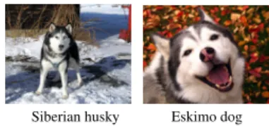
learn-Siberian husky Eskimo dog Figure 1: Semantically near-equivalent classes in ILSVRC ing that measures theWasserstein distancebetween a prediction
and the target label, with respect to a chosen metric on the out-put space. The Wasserstein distance is defined as the cost of the optimal transport plan for moving the mass in the predicted measure to match that in the target, and has been applied to a wide range of problems, including barycenter estimation [3], la-bel propagation [4], and clustering [5]. To our knowledge, this paper represents the first use of the Wasserstein distance as a loss for supervised learning.
We briefly describe a case in which the Wasserstein loss improves learning performance. The setting is a multiclass classification problem in which label noise arises from confusion of semantically near-equivalent categories. Figure 1 shows such a case from the ILSVRC, in which the categories
Siberian huskyandEskimo dog are nearly indistinguishable. We synthesize a toy version of this problem by identifying categories with points in the Euclidean plane and randomly switching the training labels to nearby classes. The Wasserstein loss yields predictions that are closer to the ground truth, robustly across all noise levels, as shown in Figure 2. The standard multiclass logistic loss is the baseline for comparison. Section E.1 in the Appendix describes the experiment in more detail. The main contributions of this paper are as follows. We formulate the problem of learning with prior knowledge of the ground metric, and propose the Wasserstein loss as an alternative to traditional information divergence-based loss functions. Specifically, we focus on empirical risk minimization (ERM) with the Wasserstein loss, and describe an efficient learning algorithm based on entropic regularization of the optimal transport problem. We also describe a novel extension to unnormalized measures that is similarly efficient to compute. We then justify ERM with the Wasserstein loss by showing a statistical learning bound. Finally, we evaluate the proposed loss on both synthetic examples and a real-world image annotation problem, demonstrating benefits for incorporating an output metric into the loss.
2
Related work
Decomposable loss functions like KL Divergence and`pdistances are very popular for
probabilis-tic [1] or vector-valued [6] predictions, as each component can be evaluated independently, often leading to simple and efficient algorithms. The idea of exploiting smoothness in the label space according to a prior metric has been explored in many different forms, including regularization [7] and post-processing with graphical models [8]. Optimal transport provides a natural distance for probability distributions over metric spaces. In [3, 9], the optimal transport is used to formulate the Wasserstein barycenter as a probability distribution with minimum total Wasserstein distance to a set of given points on the probability simplex. [4] propagates histogram values on a graph by minimizing a Dirichlet energy induced by optimal transport. The Wasserstein distance is also used to formulate a metric for comparing clusters in [5], and is applied to image retrieval [10], contour
matching [11], and many other problems [12, 13]. However, to our knowledge, this is the first time it is used as a loss function in a discriminative learning framework. The closest work to this pa-per is a theoretical study [14] of an estimator that minimizes the optimal transport cost between the empirical distribution and the estimated distribution in the setting of statistical parameter estimation.
3
Learning with a Wasserstein loss
3.1 Problem setup and notation
We consider the problem of learning a map fromX ⊂RDinto the spaceY=RK+ of measures over a finite setKof size|K| =K. AssumeK possesses a metricdK(·,·), which is called theground
metric. dK measures semantic similarity between dimensions of the output, which correspond to the elements ofK. We perform learning over a hypothesis spaceHof predictorshθ : X → Y,
parameterized byθ∈Θ. These might be linear logistic regression models, for example.
In the standard statistical learning setting, we get an i.i.d. sequence of training examples S = ((x1, y1), . . . ,(xN, yN)), sampled from an unknown joint distributionPX ×Y. Given a measure of
performance (a.k.a.risk)E(·,·), the goal is to find the predictorhθ∈ Hthat minimizes the expected
riskE[E(hθ(x), y)]. TypicallyE(·,·)is difficult to optimize directly and the joint distributionPX ×Y
is unknown, so learning is performed viaempirical risk minimization. Specifically, we solve
min hθ∈H ( ˆ ES[`(hθ(x), y) = 1 N N X i=1 `(hθ(xi), yi) ) (1)
with a loss function`(·,·)acting as a surrogate ofE(·,·). 3.2 Optimal transport and the exact Wasserstein loss
Information divergence-based loss functions are widely used in learning with probability-valued out-puts. Along with other popular measures like Hellinger distance andχ2distance, these divergences treat the output dimensions independently, ignoring any metric structure onK.
Given a cost functionc : K × K → R, theoptimal transportdistance [15] measures the cheapest way to transport the mass in probability measureµ1to match that inµ2:
Wc(µ1, µ2) = inf
γ∈Π(µ1,µ2)
Z
K×K
c(κ1, κ2)γ(dκ1, dκ2) (2) whereΠ(µ1, µ2)is the set of joint probability measures onK×Khavingµ1andµ2as marginals. An important case is that in which the cost is given by a metricdK(·,·)or itsp-th powerdpK(·,·)withp≥
1. In this case, (2) is called aWasserstein distance[16], also known as theearth mover’s distance
[10]. In this paper, we only work with discrete measures. In the case of probability measures, these are histograms in the simplex∆K. When the ground truthy and the output of hboth lie in the simplex∆K, we can define a Wasserstein loss.
Definition 3.1(Exact Wasserstein Loss). For anyhθ∈ H,hθ:X →∆K, lethθ(κ|x) =hθ(x)κbe the predicted value at elementκ∈ K, given inputx∈ X. Lety(κ)be the ground truth value forκ given by the corresponding labely. Then we define theexact Wasserstein lossas
Wpp(h(·|x), y(·)) = inf
T∈Π(h(x),y)hT, Mi (3)
whereM ∈RK+×Kis the distance matrixMκ,κ0 =dp
K(κ, κ0), and the set of valid transport plans is
Π(h(x), y) ={T ∈RK+×K :T1=h(x), T>1=y} (4)
where1is the all-one vector.
Wpp is the cost of the optimal plan for transporting the predicted mass distributionh(x)to match
the target distributiony. The penalty increases as more mass is transported over longer distances, according to the ground metricM.
Algorithm 1Gradient of the Wasserstein loss
Givenh(x),y,λ,K. (γa,γbifh(x),yunnormalized.)
u←1
whileuhas not convergeddo
u← h(x) K yK>u ifh(x),ynormalized h(x)γaλ+1γaλ K yK>u γbλ γbλ+1 γaλ+1γaλ ifh(x),yunnormalized end while Ifh(x),yunnormalized:v←yγbλγbλ+1 K>u γbλ γbλ+1 ∂Wp p/∂h(x)← logu λ − logu>1 λK 1 ifh(x),ynormalized γa(1−(diag(u)Kv)h(x)) ifh(x),yunnormalized
4
Efficient optimization via entropic regularization
To do learning, we optimize the empirical risk minimization functional (1) by gradient descent. Doing so requires evaluating a descent direction for the loss, with respect to the predictionsh(x). Unfortunately, computing a subgradient of the exact Wasserstein loss (3), is quite costly, as follows. The exact Wasserstein loss (3) is a linear program and a subgradient of its solution can be computed using Lagrange duality. The dual LP of (3) is
dWp
p(h(x), y) = sup
α,β∈CM
α>h(x) +β>y, CM ={(α, β)∈RK×K:ακ+βκ0 ≤Mκ,κ0}. (5)
As (3) is a linear program, at an optimum the values of the dual and the primal are equal (see, e.g. [17]), hence the dual optimalαis a subgradient of the loss with respect to its first argument. Computingαis costly, as it entails solving a linear program withO(K2)contraints, withKbeing the dimension of the output space. This cost can be prohibitive when optimizing by gradient descent. 4.1 Entropic regularization of optimal transport
Cuturi [18] proposes a smoothed transport objective that enables efficient approximation of both the transport matrix in (3) and the subgradient of the loss. [18] introduces an entropic regularization term that results in a strictly convex problem:
λWp p(h(·|x), y(·)) = inf T∈Π(h(x),y)hT, Mi − 1 λH(T), H(T) =− X κ,κ0 Tκ,κ0logTκ,κ0. (6)
Importantly, the transport matrix that solves (6) is adiagonal scalingof a matrixK=e−λM−1:
T∗=diag(u)Kdiag(v) (7)
foru=eλαandv=eλβ, whereαandβare the Lagrange dual variables for (6).
Identifying such a matrix subject to equality constraints on the row and column sums is exactly a
matrix balancingproblem, which is well-studied in numerical linear algebra and for which efficient iterative algorithms exist [19]. [18] and [3] use the well-known Sinkhorn-Knopp algorithm. 4.2 Extending smoothed transport to the learning setting
When the output vectorsh(x)andy lie in the simplex, (6) can be used directly in place of (3), as (6) can approximate the exact Wasserstein distance closely for large enoughλ[18]. In this case, the gradientαof the objective can be obtained from the optimal scaling vectoruasα= logλu−logu>1
λK 1.
1 A Sinkhorn iteration for the gradient is given in Algorithm 1.
1Note thatαis only defined up to a constant shift: any upscaling of the vectorucan be paired with a corresponding downscaling of the vectorv(and vice versa) without altering the matrixT∗. The choiceα=
logu λ −
logu>1
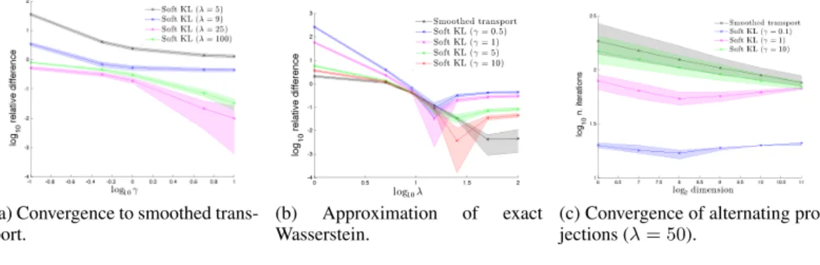
(a) Convergence to smoothed trans-port.
(b) Approximation of exact Wasserstein.
(c) Convergence of alternating pro-jections (λ= 50).
Figure 3: The relaxed transport problem (8) for unnormalized measures.
For many learning problems, however, a normalized output assumption is unnatural. In image seg-mentation, for example, the target shape is not naturally represented as a histogram. And even when the prediction and the ground truth are constrained to the simplex, the observed label can be subject to noise that violates the constraint.
There is more than one way to generalize optimal transport to unnormalized measures, and this is a subject of active study [20]. We will develop here a novel objective that deals effectively with the difference in total mass betweenh(x)andywhile still being efficient to optimize.
4.3 Relaxed transport
We propose a novel relaxation that extends smoothed transport to unnormalized measures. By re-placing the equality constraints on the transport marginals in (6) with soft penalties with respect to KL divergence, we get an unconstrained approximate transport problem. The resulting objective is:
λ,γa,γbW KL(h(·|x), y(·)) = min T∈RK+×K hT, Mi −1 λH(T) +γaKLf(T1kh(x)) +γbKLf T >1ky (8)
where KLf(wkz) = w>log(wz)−1>w +1>z is the generalized KL divergence between
w, z∈RK+. Hererepresents element-wise division. As with the previous formulation, the optimal transport matrix with respect to (8) is a diagonal scaling of the matrixK.
Proposition 4.1. The transport matrixT∗ optimizing(8)satisfiesT∗ =diag(u)Kdiag(v), where u= (h(x)T∗1)γaλ,v= y(T∗)>1γbλ
, andK=e−λM−1.
And the optimal transport matrix is a fixed point for a Sinkhorn-like iteration.2
Proposition 4.2. T∗=diag(u)Kdiag(v)optimizing(8)satisfies: i)u=h(x)γaλ+1γaλ (Kv)− γaλ γaλ+1,
and ii)v=yγbλγbλ+1 K>u− γbλ
γbλ+1, whererepresents element-wise multiplication.
Unlike the previous formulation, (8) is unconstrained with respect toh(x). The gradient is given by ∇h(x)WKL(h(·|x), y(·)) =γa(1−T∗1h(x)). The iteration is given in Algorithm 1.
When restricted to normalized measures, the relaxed problem (8) approximates smoothed transport (6). Figure 3a shows, for normalizedh(x)andy, the relative distance between the values of (8) and (6)3. Forλlarge enough, (8) converges to (6) asγ
aandγbincrease.
(8) also retains two properties of smoothed transport (6). Figure 3b shows that, for normalized outputs, the relaxed loss converges to the unregularized Wasserstein distance asλ,γaandγbincrease
4. And Figure 3c shows that convergence of the iterations in (4.2) is nearly independent of the dimensionKof the output space.
2
Note that, although the iteration suggested by Proposition 4.2 is observed empirically to converge (see Figure 3c, for example), we have not proven a guarantee that it will do so.
3In figures 3a-c,h(x),yandM are generated as described in [18] section 5. In 3a-b,h(x)andyhave dimension256. In 3c, convergence is defined as in [18]. Shaded regions are95%intervals.
4
0 1 2 3 4 p-th norm 0.08 0.10 0.12 0.14 0.16 0.18 0.20 P oster ior Probability 0 1 2 3
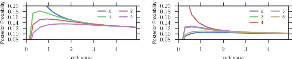
(a) Posterior predictions for images of digit 0.
0 1 2 3 4 p-th norm 0.08 0.10 0.12 0.14 0.16 0.18 0.20 P oster ior Probability 2 3 4 5 6
(b) Posterior predictions for images of digit 4. Figure 4: MNIST example. Each curve shows the predicted probability for one digit, for models trained with differentpvalues for the ground metric.
5
Statistical Properties of the Wasserstein loss
LetS= ((x1, y1), . . . ,(xN, yN))be i.i.d. samples andhθˆbe the empirical risk minimizer
hθˆ= argmin hθ∈H ( ˆ ES Wpp(hθ(·|x), y) = 1 N N X i=1 Wpp(hxθ(·|xi), yi) ) .
Further assumeH=s◦ Hois the composition of a softmaxsand a base hypothesis spaceHoof
functions mapping intoRK. The softmax layer outputs a prediction that lies in the simplex∆K. Theorem 5.1. Forp= 1, and anyδ >0, with probability at least1−δ, it holds that
EW11(hθˆ(·|x), y)≤ inf hθ∈H EW11(hθ(·|x), y) + 32KCMRN(Ho) + 2CM r log(1/δ) 2N (9)
with the constantCM = maxκ,κ0Mκ,κ0. RN(Ho)is theRademacher complexity[22] measuring the complexity of the hypothesis spaceHo.
The Rademacher complexityRN(Ho)for commonly used models like neural networks and kernel
machines [22] decays with the training set size. This theorem guarantees that the expected Wasser-stein loss of the empirical risk minimizer approaches the best achievable loss forH.
As an important special case, minimizing the empirical risk with Wasserstein loss is also good for multiclass classification. Lety=eκbe the “one-hot” encoded label vector for the groundtruth class.
Proposition 5.2. In the multiclass classification setting, forp= 1and anyδ >0, with probability at least1−δ, it holds that
Ex,κ dK(κθˆ(x), κ) ≤ inf hθ∈H KE[W11(hθ(x), y)] + 32K2CMRN(Ho) + 2CMK r log(1/δ) 2N (10)
where the predictor isκθˆ(x) = argmaxκhθˆ(κ|x), withhθˆbeing the empirical risk minimizer. Note that instead of the classification errorEx,κ[1{κθˆ(x) 6= κ}], we actually get a bound on the expected semantic distance between the prediction and the groundtruth.
6
Empirical study
6.1 Impact of the ground metric
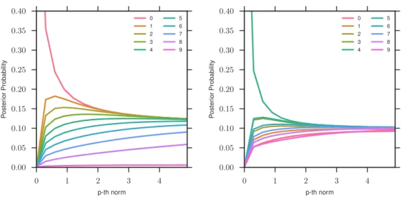
In this section, we show that the Wasserstein loss encourages smoothness with respect to an artificial metric on the MNIST handwritten digit dataset. This is a multi-class classification problem with output dimensions corresponding to the 10 digits, and we apply a ground metricdp(κ, κ0) =|κ− κ0|p, whereκ, κ0 ∈ {0, . . . ,9}andp∈[0,∞). This metric encourages the recognized digit to be
numericallyclose to the true one. We train a model independently for each value ofpand plot the average predicted probabilities of the different digits on the test set in Figure 4.
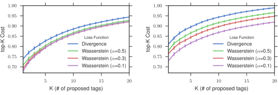
5 10 15 20 K (# of proposed tags) 0.70 0.75 0.80 0.85 0.90 0.95 1.00 top-K
Cost Loss Function
Divergence Wasserstein (α=0.5) Wasserstein (α=0.3) Wasserstein (α=0.1)
(a) Original Flickr tags dataset.
5 10 15 20 K (# of proposed tags) 0.70 0.75 0.80 0.85 0.90 0.95 1.00 top-K
Cost Loss Function
Divergence Wasserstein (α=0.5) Wasserstein (α=0.3) Wasserstein (α=0.1)
(b) Reduced-redundancy Flickr tags dataset. Figure 5: Top-K cost comparison of the proposed loss (Wasserstein) and the baseline (Divergence). Note that asp → 0, the metric approaches the0−1metric d0(κ, κ0) = 1κ6=κ0, which treats all
incorrect digits as being equally unfavorable. In this case, as can be seen in the figure, the predicted probability of the true digit goes to 1 while the probability for all other digits goes to 0. Asp
increases, the predictions become more evenly distributed over the neighboring digits, converging to a uniform distribution asp→ ∞5.
6.2 Flickr tag prediction
We apply the Wasserstein loss to a real world multi-label learning problem, using the recently re-leased Yahoo/Flickr Creative Commons 100M dataset [23]. 6 Our goal istag prediction: we select 1000 descriptive tags along with two random sets of 10,000 images each, associated with these tags, for training and testing. We derive a distance metric between tags by usingword2vec[24] to embed the tags as unit vectors, then taking their Euclidean distances. To extract image features we useMatConvNet[25]. Note that the set of tags is highly redundant and often many semantically equivalent or similar tags can apply to an image. The images are also partially tagged, as different users may prefer different tags. We therefore measure the prediction performance by thetop-K cost, defined asCK= 1/KP
K
k=1minjdK(ˆκk, κj), where{κj}is the set of groundtruth tags, and{ˆκk}
are the tags with highest predicted probability. The standard AUC measure is also reported. We find that a linear combination of the Wasserstein lossWp
p and the standard multiclass logistic loss
KLyields the best prediction results. Specifically, we train a linear model by minimizingWp
p+αKL
on the training set, whereαcontrols the relative weight ofKL. Note thatKL taken alone is our baseline in these experiments. Figure 5a shows the top-K cost on the test set for the combined loss and the baselineKL loss. We additionally create a second dataset by removing redundant labels from the original dataset: this simulates the potentially more difficult case in which a single user tags each image, by selecting one tag to apply from amongst each cluster of applicable, semantically similar tags. Figure 3b shows that performance for both algorithms decreases on the harder dataset, while the combined Wasserstein loss continues to outperform the baseline.
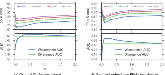
In Figure 6, we show the effect on performance of varying the weightαon the KL loss. We observe that the optimum of the top-Kcost is achieved when the Wasserstein loss is weighted more heavily than at the optimum of the AUC. This is consistent with a semantic smoothing effect of Wasserstein, which during training will favor mispredictions that are semantically similar to the ground truth, sometimes at the cost of lower AUC7. We finally show two selected images from the test set in Figure 7. These illustrate cases in which both algorithms make predictions that are semantically relevant, despite overlapping very little with the ground truth. The image on the left shows errors made by both algorithms. More examples can be found in the appendix.
5To avoid numerical issues, we scale down the ground metric such that all of the distance values are in the interval[0,1).
6
The dataset used here is available athttp://cbcl.mit.edu/wasserstein. 7
The Wasserstein loss can achieve a similar trade-off by choosing the metric parameterp, as discussed in Section 6.1. However, the relationship betweenpand the smoothing behavior is complex and it can be simpler to implement the trade-off by combining with theKLloss.
0.0 0.5 1.0 1.5 2.0 0.65 0.70 0.75 0.80 0.85 0.90 0.95 T op-K cost K = 1 K = 2 K = 3 K = 4 0.0 0.5 1.0 1.5 2.0 α 0.54 0.56 0.58 0.60 0.62 0.64 A UC Wasserstein AUC Divergence AUC
(a) Original Flickr tags dataset.
0.0 0.5 1.0 1.5 2.0 0.65 0.70 0.75 0.80 0.85 0.90 0.95 T op-K cost K = 1 K = 2 K = 3 K = 4 0.0 0.5 1.0 1.5 2.0 α 0.54 0.56 0.58 0.60 0.62 0.64 A UC Wasserstein AUC Divergence AUC
(b) Reduced-redundancy Flickr tags dataset. Figure 6: Trade-off between semantic smoothness and maximum likelihood.
(a)Flickr user tags: street, parade, dragon;our proposals: people, protest, parade;baseline pro-posals: music, car, band.
(b)Flickr user tags: water, boat, reflection, sun-shine;our proposals: water, river, lake, summer; baseline proposals: river, water, club, nature. Figure 7: Examples of images in the Flickr dataset. We show the groundtruth tags and as well as tags proposed by our algorithm and the baseline.
7
Conclusions and future work
In this paper we have described a loss function for learning to predict a non-negative measure over a finite set, based on the Wasserstein distance. Although optimizing with respect to the exact Wasser-stein loss is computationally costly, an approximation based on entropic regularization is efficiently computed. We described a learning algorithm based on this regularization and we proposed a novel extension of the regularized loss to unnormalized measures that preserves its efficiency. We also described a statistical learning bound for the loss. The Wasserstein loss can encourage smoothness of the predictions with respect to a chosen metric on the output space, and we demonstrated this property on a real-data tag prediction problem, showing improved performance over a baseline that doesn’t incorporate the metric.
An interesting direction for future work may be to explore the connection between the Wasserstein loss and Markov random fields, as the latter are often used to encourage smoothness of predictions, via inference at prediction time.
References
[1] Jonathan Long, Evan Shelhamer, and Trevor Darrell. Fully convolutional networks for semantic segmen-tation.CVPR (to appear), 2015.
[2] Olga Russakovsky, Jia Deng, Hao Su, Jonathan Krause, Sanjeev Satheesh, Sean Ma, Zhiheng Huang, Andrej Karpathy, Aditya Khosla, Michael Bernstein, Alexander C. Berg, and Li Fei-Fei. ImageNet Large Scale Visual Recognition Challenge.International Journal of Computer Vision (IJCV), 2015.
[3] Marco Cuturi and Arnaud Doucet. Fast Computation of Wasserstein Barycenters.ICML, 2014.
[4] Justin Solomon, Raif M Rustamov, Leonidas J Guibas, and Adrian Butscher. Wasserstein Propagation for Semi-Supervised Learning. InICML, pages 306–314, 2014.
[5] Michael H Coen, M Hidayath Ansari, and Nathanael Fillmore. Comparing Clusterings in Space. ICML, pages 231–238, 2010.
[6] Lorenzo Rosasco Mauricio A. Alvarez and Neil D. Lawrence. Kernels for vector-valued functions: A review.Foundations and Trends in Machine Learning, 4(3):195–266, 2011.
[7] Leonid I Rudin, Stanley Osher, and Emad Fatemi. Nonlinear total variation based noise removal algo-rithms.Physica D: Nonlinear Phenomena, 60(1):259–268, 1992.
[8] Liang-Chieh Chen, George Papandreou, Iasonas Kokkinos, Kevin Murphy, and Alan L Yuille. Semantic image segmentation with deep convolutional nets and fully connected crfs. InICLR, 2015.
[9] Marco Cuturi, Gabriel Peyr´e, and Antoine Rolet. A Smoothed Dual Approach for Variational Wasserstein Problems.arXiv.org, March 2015.
[10] Yossi Rubner, Carlo Tomasi, and Leonidas J Guibas. The earth mover’s distance as a metric for image retrieval.IJCV, 40(2):99–121, 2000.
[11] Kristen Grauman and Trevor Darrell. Fast contour matching using approximate earth mover’s distance. InCVPR, 2004.
[12] S Shirdhonkar and D W Jacobs. Approximate earth mover’s distance in linear time. InCVPR, 2008. [13] Herbert Edelsbrunner and Dmitriy Morozov. Persistent homology: Theory and practice. InProceedings
of the European Congress of Mathematics, 2012.
[14] Federico Bassetti, Antonella Bodini, and Eugenio Regazzini. On minimum kantorovich distance estima-tors.Stat. Probab. Lett., 76(12):1298–1302, 1 July 2006.
[15] C´edric Villani.Optimal Transport: Old and New. Springer Berlin Heidelberg, 2008.
[16] Vladimir I Bogachev and Aleksandr V Kolesnikov. The Monge-Kantorovich problem: achievements, connections, and perspectives.Russian Math. Surveys, 67(5):785, 10 2012.
[17] Dimitris Bertsimas, John N. Tsitsiklis, and John Tsitsiklis. Introduction to Linear Optimization. Athena Scientific, Boston, third printing edition, 1997.
[18] Marco Cuturi. Sinkhorn Distances: Lightspeed Computation of Optimal Transport.NIPS, 2013. [19] Philip A Knight and Daniel Ruiz. A fast algorithm for matrix balancing. IMA Journal of Numerical
Analysis, 33(3):drs019–1047, October 2012.
[20] Lenaic Chizat, Gabriel Peyr´e, Bernhard Schmitzer, and Franc¸ois-Xavier Vialard. Unbalanced Optimal Transport: Geometry and Kantorovich Formulation.arXiv.org, August 2015.
[21] Ofir Pele and Michael Werman. Fast and robust Earth Mover’s Distances.ICCV, pages 460–467, 2009. [22] Peter L Bartlett and Shahar Mendelson. Rademacher and gaussian complexities: Risk bounds and
struc-tural results.JMLR, 3:463–482, March 2003.
[23] Bart Thomee, David A. Shamma, Gerald Friedland, Benjamin Elizalde, Karl Ni, Douglas Poland, Damian Borth, and Li-Jia Li. The new data and new challenges in multimedia research. arXiv preprint arXiv:1503.01817, 2015.
[24] Tomas Mikolov, Ilya Sutskever, Kai Chen, Greg S Corrado, and Jeff Dean. Distributed representations of words and phrases and their compositionality. InNIPS, 2013.
[25] A. Vedaldi and K. Lenc. MatConvNet – Convolutional Neural Networks for MATLAB. CoRR, abs/1412.4564, 2014.
[26] M. Ledoux and M. Talagrand. Probability in Banach Spaces: Isoperimetry and Processes. Classics in Mathematics. Springer Berlin Heidelberg, 2011.
[27] Clark R. Givens and Rae Michael Shortt. A class of wasserstein metrics for probability distributions.
A
Relaxed transport
Equation (8) gives the relaxed transport objective as
λ,γa,γbW KL(h(·|x), y(·)) = min T∈RK+×K hT, Mi −1 λH(T) +γaKLf(T1kh(x)) +γbKLf T >1ky withKLf(wkz) =w>log(wz)−1>w+1>z.
Proof of Proposition 4.1. The first order condition forT∗optimizing (8) is
Mij+ 1 λ logT ∗ ij+ 1 +γa(logT∗1h(x))i+γb log(T∗)>1y j = 0.
⇒logTij∗ +γaλlog (T∗1h(xi))i+γbλlog (T∗)>1yjj=−λMij−1
⇒Tij∗(T∗1h(x))γaλ i (T ∗)>1yγbλ j = exp (−λMij−1) ⇒Tij∗ = (h(x)T∗1)γaλ i y(T ∗)>1γbλ j exp (−λMij−1)
HenceT∗(if it exists) is a diagonal scaling ofK= exp (−λM −1).
Proof of Proposition 4.2. Let u = (h(x)T∗1)γaλ and v = y(T∗)>1γbλ
, so T∗ = diag(u)Kdiag(v). We have
T∗1=diag(u)Kv
⇒(T∗1)γaλ+1=h(x)γaλKv where we substituted the expression foru. Re-writingT∗1,
(diag(u)Kv)γaλ+1=diag(h(x)γaλ)Kv ⇒uγaλ+1=h(x)γaλ(Kv)−γaλ
⇒u=h(x)γaλ+1γaλ (Kv)− γaλ γaλ+1.
A symmetric argument shows thatv=yγbλγbλ+1(K>u)− γbλ γbλ+1.
B
Statistical Learning Bounds
We establish the proof of Theorem 5.1 in this section. For simpler notation, for a sequenceS = ((x1, y1), . . . ,(xN, yN))of i.i.d. training samples, we denote the empirical riskRˆSand riskRas
ˆ RS(hθ) = ˆES Wpp(hθ(·|x), y(·)) , R(hθ) =EWpp(hθ(·|x), y(·)) (11) Lemma B.1. Let hθˆ, hθ∗ ∈ H be the minimizer of the empirical riskRˆS and expected risk R, respectively. Then
R(hθˆ)≤R(hθ∗) + 2 sup
h∈H
|R(h)−RˆS(h)|
Proof. By the optimality ofhθˆforRˆS, R(hθˆ)−R(hθ∗) =R(hˆ θ)−RˆS(hθˆ) + ˆRS(hθˆ)−R(hθ∗) ≤R(hθˆ)−RˆS(hθˆ) + ˆRS(hθ∗)−R(hθ∗) ≤2 sup h∈H |R(h)−RˆS(h)|
Therefore, to bound the risk for hθˆ, we need to establish uniform concentration bounds for the Wasserstein loss. Towards that goal, we define a space of loss functions induced by the hypothesis spaceHas
L=`θ: (x, y)7→Wpp(hθ(·|x), y(·)) :hθ∈ H (12)
The uniform concentration will depends on the “complexity” ofL, which is measured by the empir-icalRademacher complexitydefined below.
Definition B.2 (Rademacher Complexity [22]). LetG be a family of mapping from Z toR, and S = (z1, . . . , zN)a fixed sample fromZ. Theempirical Rademacher complexityofGwith respect toSis defined as ˆ RS(G) =Eσ " sup g∈G 1 N n X i=1 σig(zi) # (13)
where σ = (σ1, . . . , σN), with σi’s independent uniform random variables taking values in
{+1,−1}. σi’s are called the Rademacher random variables. TheRademacher complexityis de-fined by taking expectation with respect to the samplesS,
RN(G) =ES h ˆ RS(G) i (14) Theorem B.3. For anyδ >0, with probability at least1−δ, the following holds for all`θ∈ L,
E[`θ]−EˆS[`θ]≤2RN(L) +
r
C2
Mlog(1/δ)
2N (15)
with the constantCM = maxκ,κ0Mκ,κ0.
By the definition ofL,E[`θ] =R(hθ)andEˆS[`θ] = ˆRS[hθ]. Therefore, this theorem provides a
uniform control for the deviation of the empirical risk from the risk.
Theorem B.4(McDiarmid’s Inequality). LetS ={X1, . . . , XN} ⊂X beN i.i.d. random vari-ables. Assume there existsC >0such thatf :XN →
Rsatisfies the following stability condition
|f(x1, . . . , xi, . . . , xN)−f(x1, . . . , x0i, . . . , xN)| ≤C (16) for alli= 1, . . . , N and anyx1, . . . , xN, x0i ∈X. Then for anyε >0, denotingf(X1, . . . , XN) byf(S), it holds that P(f(S)−E[f(S)]≥ε)≤exp − 2ε 2 N C2 (17)
Lemma B.5. Let the constantCM = maxκ,κ0Mκ,κ0, then0≤Wpp(·,·)≤CM.
Proof. For anyh(·|x)andy(·), letT∗ ∈ Π(h(x), y)be the optimal transport plan that solves (3), then
Wpp(h(x), y) =hT∗, Mi ≤CM
X
κ,κ0
Tκ,κ0 =CM
Proof of Theorem B.3. For any`θ ∈ L, note the empirical expectation is the empirical risk of the
correspondinghθ: ˆ ES[`θ] = 1 N N X i=1 `θ(xi, yi) = 1 N N X i=1 Wpp(hθ(·|xi), yi(·)) = ˆRS(hθ) Similarly,E[`θ] =R(hθ). Let Φ(S) = sup `∈LE [`]−EˆS[`] (18)
LetS0beSwith thei-th sample replaced by(x0i, yi0), by Lemma B.5, it holds that
Φ(S)−Φ(S0)≤sup `∈L ˆ ES0[`]−EˆS[`] = sup hθ∈H Wpp(hθ(x0i), y0i)−W p p(hθ(xi), yi) N ≤ CM N
Similarly, we can showΦ(S0)−Φ(S)≤CM/N, thus|Φ(S0)−Φ(S)| ≤CM/N. By Theorem B.4,
for anyδ >0, with probability at least1−δ, it holds that
Φ(S)≤E[Φ(S)] +
r
C2
Mlog(1/δ)
2N (19)
To boundE[Φ(S)], by Jensen’s inequality,
ES[Φ(S)] =ES sup `∈LE [`]−EˆS[`] =ES sup `∈LE S0 h ˆ ES0[`]−EˆS[`] i ≤ES,S0 sup `∈L ˆ ES0[`]−EˆS[`]
HereS0 is another sequence of i.i.d. samples, usually calledghost samples, that is only used for analysis. Now we introduce the Rademacher variablesσi, since the role ofSandS0are completely
symmetric, it follows ES[Φ(S)]≤ES,S0,σ " sup `∈L 1 N N X i=1 σi(`(x0i, yi0)−`(xi, yi)) # ≤ES0,σ " sup `∈L 1 N N X i=1 σi`(x0i, y 0 i) # +ES,σ " sup `∈L 1 N N X i=1 −σi`(xi, yi) # =ES h ˆ RS(L) i +ES0 h ˆ RS0(L) i = 2RN(L)
The conclusion follows by combing (18) and (19).
To finish the proof of Theorem 5.1, we combine Lemma B.1 and Theorem B.3, and relateRN(L)
toRN(H)via the following generalized Talagrand’s lemma [26].
Lemma B.6. LetF be a class of real functions, andH ⊂ F =F1×. . .× FK be aK-valued function class. Ifm : RK → Ris aLm-Lipschitz function and m(0) = 0, thenRˆS(m◦ H) ≤
2LmP
K
k=1RˆS(Fk).
Theorem B.7(Theorem 6.15 of [15]). Letµandνbe two probability measures on a Polish space
(K, dK). Letp∈[1,∞)andκ0∈ K. Then
Wp(µ, ν)≤21/p 0Z K dK(κ0, κ)d|µ−ν|(κ) 1/p , 1 p+ 1 p0 = 1 (20)
Corollary B.8. The Wasserstein loss is Lipschitz continuous in the sense that for anyhθ∈ H, and any(x, y)∈ X × Y,
Wpp(hθ(·|x), y)≤2p−1CM
X
κ∈K
|hθ(κ|x)−y(κ)| (21) In particular, whenp= 1, we have
W11(hθ(·|x), y)≤CM
X
κ∈K
|hθ(κ|x)−y(κ)| (22)
We cannot apply Lemma B.6 directly to the Wasserstein loss class, because the Wasserstein loss is only defined on probability distributions, so0is not a valid input. To get around this problem, we assume the hypothesis spaceHused in learning is of the form
H={s◦ho:ho∈ Ho} (23)
whereHois a function class that maps into
RK, and sis the softmax function defined ass(o) =
(s1(o), . . . ,sK(o)), with sk(o) = eok P jeoj , k= 1, . . . , K (24)
The softmax layer produce a valid probability distribution from arbitrary input, and this is consistent with commonly used models such as Logistic Regression and Neural Networks. By working with thelogof the groundtruth labels, we can also add a softmax layer to the labels.
Lemma B.9(Proposition 2 of [27]). The Wasserstein distancesWp(·,·)are metrics on the space of probability distributions ofK, for all1≤p≤ ∞.
Proposition B.10. The mapι:RK×RK →Rdefined byι(y, y0) =W11(s(y),s(y0))satisfies |ι(y, y0)−ι(¯y,y¯0)| ≤4CMk(y, y0)−(¯y,y¯0)k2 (25) for any(y, y0),(¯y,y¯0)∈RK×
RK. Andι(0,0) = 0.
Proof. For any(y, y0),(¯y,y¯0)∈RK×RK, by Lemma B.9, we can use triangle inequality on the
Wasserstein loss,
|ι(y, y0)−ι(¯y,y¯0)|=|ι(y, y0)−ι(¯y, y0) +ι(¯y, y0)−ι(¯y,y¯0)| ≤ι(y,y¯) +ι(y0,y¯0)
Following Corollary B.8, it continues as
|ι(y, y0)−ι(¯y,y¯0)| ≤CM(ks(y)−s(¯y)k1+ks(y0)−s(¯y0)k1) (26)
Note for eachk= 1, . . . , K, the gradient∇ysksatisfies
k∇yskk2= ∂sk ∂yj K j=1 2 = (δkjsk−sksj) K j=1 2= v u u ts2k K X j=1 s2 j+s2k(1−2sk) (27)
By mean value theorem,∃α∈[0,1], such that foryθ=αy+ (1−α)¯y, it holds that
ks(y)−s(¯y)k1= K X k=1 h∇ysk|y=yαk, y−y¯i ≤ K X k=1 k∇ysk|y=yαkk2ky−y¯k2≤2ky−y¯k2
because by (27), and the fact thatqP
js2j ≤ P jsj = 1and √ a+b ≤√a+√bfora, b≥0, it holds K X k=1 k∇yskk2= X k:sk≤1/2 k∇yskk2+ X k:sk>1/2 k∇yskk2 ≤ X k:sk≤1/2 sk+sk √ 1−2sk + X k:sk>1/2 sk≤ K X k=1 2sk= 2
Similarly, we haveks(y0)−s(¯y0)k1≤2ky0−y¯0k2, so from (26), we know |ι(y, y0)−ι(¯y,y¯0)| ≤2CM(ky−y¯k2+ky0−y¯0k2)≤2
√
2CM ky−y¯k22+ky0−y¯0k22 1/2
then (25) follows immediately. The second conclusion follows trivially assmaps the zero vector to a uniform distribution.
Proof of Theorem 5.1. Consider the loss function space preceded with a softmax layer L={ιθ: (x, y)7→W11(s(h o θ(x)),s(y)) :h o θ∈ H o }
We apply Lemma B.6 to the 4CM-Lipschitz continuous function ι in Proposition B.10 and the
function space Ho×. . .× Ho | {z } Kcopies × I ×. . .× I | {z } Kcopies withIa singleton function space with only the identity map. It holds
ˆ RS(L)≤8CM KRˆS(Ho) +KRˆS(I) = 8KCMRˆS(Ho) (28)
because for the identity map, and a sampleS= (y1, . . . , yN), we can calculate ˆ RS(I) =Eσ " sup f∈I 1 N N X i=1 σif(yi) # =Eσ " 1 N N X i=1 σiyi # = 0
C
Connection with multiclass classification
Proof of Proposition 5.2. Given that the label is a “one-hot” vectory=eκ, the set of transport plans
(4) degenerates. Specifically, the constraintT>1=eκmeans that only theκ-th column ofT can
be non-zero. Furthermore, the constraintT1=hθˆ(·|x)ensures that theκ-th column ofT actually equalshθˆ(·|x). In other words, the setΠ(hθˆ(·|x),eκ)contains only one feasible transport plan, so
(3) can be computed directly as
Wpp(hθˆ(·|x),eκ) = X κ0∈K Mκ0,κhˆ θ(κ 0|x) = X κ0∈K dpK(κ0, κ)hθˆ(κ0|x) Now letκˆ= argmaxκhθˆ(κ|x)be the prediction, we have
hθˆ(ˆκ|x) = 1− X κ6=ˆκ hθˆ(κ|x)≥1− X κ6=ˆκ hθˆ(ˆκ|x) = 1−(K−1)hθˆ(ˆκ|x) Therefore,hθˆ(ˆκ|x)≥1/K, so Wpp(hθˆ(·|x),eκ)≥dpK(ˆκ, κ)hθˆ(ˆκ|x)≥dpK(ˆκ, κ)/K The conclusion follows by applying Theorem 5.1 withp= 1.
D
Algorithmic Details of Learning with a Wasserstein Loss
In Section 5, we describe the statistical generalization properties of learning with a Wasserstein loss function via empirical risk minimization on a general space of classifiersH. In all the empirical studies presented in the paper, we use the space of linear logistic regression classifiers, defined by
H= hθ(x) = exp(θ> kx) PK j=1exp(θ>jx) !K k=1 :θk ∈RD, k= 1, ..., K
We use stochastic gradient descent with a mini-batch size of 100 samples to optimize the empirical risk, with a standard regularizer0.0005PK
k=1kθkk
2
2 on the weights. The algorithm is described in Algorithm 2, where WASSERSTEINis a sub-routine that computes the Wasserstein loss and its subgradient via the dual solution as described in Algorithm 1. We always run the gradient descent for a fixed number of 100,000 iterations for training.
Algorithm 2SGD Learning of Linear Logistic Model with Wasserstein Loss Initθ1randomly.
fort= 1, . . . , T do
Sample mini-batchDt= (x
1, y1), . . . ,(xn, yn)from the training set.
Compute Wasserstein subgradient∂Wp
p/∂hθ|θt ←WASSERSTEIN(Dt, hθt(·)). Compute parameter subgradient∂Wpp/∂θ|θt= (∂hθ/∂θ)(∂Wpp/∂hθ)|θt Update parameterθt+1←θt−η
t∂Wpp/∂θ|θt
end for
Note that the same training algorithm can easily be extended from training a linear logistic regres-sion model to a multi-layer neural network model, by cascading the chain-rule in the subgradient computation.
E
Empirical study
E.1 Noisy label exampleWe simulate the phenomenon of label noise arising from confusion of semantically similar classes as follows. Consider a multiclass classification problem, in which the labels correspond to the vertices on aD×Dlattice on the 2D plane. The Euclidean distance inR2is used to measure the
(a) Noise level 0.1 (b) Noise level 0.5 Figure 8: Illustration of training samples on a 3x3 lattice with different noise levels.
semantic similarity between labels. The observations for each category are samples from an isotropic Gaussian distribution centered at the corresponding vertex. Given a noise levelt, we choose with probabilitytto flip the label for each training sample to one of the neighboring categories8, chosen uniformly at random. Figure 8 shows the training set for a3×3lattice with noise levelst= 0.1and
t= 0.5, respectively.
Figure 2 is generated as follows. We repeat 10 times for noise levels t = 0.1,0.2, . . . ,0.9 and
D= 3,4, . . . ,7. We train a multiclass linear logistic regression classifier (as described in section D of the Appendix) using either the standardKL-divergence loss9or the proposed Wasserstein loss10. The performance is measured by the mean Euclidean distance in the plane between the predicted class and the true class, on the test set. Figure 2 compares the performance of the two loss functions. E.2 Full figure for the MNIST example
The full version of Figure 4 from Section 6.1 is shown in Figure 9. E.3 Details of the Flickr tag prediction experiment
From the tags in the Yahoo Flickr Creative Commons dataset, we filtered out those not occurring in the WordNet11 database, as well those whose dominant lexical category was ”noun.location” or ”noun.time.” We also filtered out by hand nouns referring to geographical location or nationality, proper nouns, numbers, photography-specific vocabulary, and several words not generally descrip-tive of visual content (such as ”annual” and ”demo”). From the remainder, the 1000 most frequently occurring tags were used.
We list some of the 1000 selected tags here. The 50 most frequently occurring tags:travel, square, wedding, art, flower, music, nature, party, beach, family, people, food, tree, summer, water, concert, winter, sky, snow, street, portrait, architecture, car, live, trip, friend, cat, sign, garden, mountain, bird, sport, light, museum, animal, rock, show, spring, dog, film, blue, green, road, girl, event, red,
8
Connected vertices on the lattice are considered neighbors, and the Euclidean distance between neighbors is set to 1.
9
This corresponds to maximum likelihood estimation of the logistic regression model.
10In this special case, this corresponds to weighted maximum likelihood estimation, c.f. Section C. 11http://wordnet.princeton.edu
0 1 2 3 4 p-th norm 0.00 0.05 0.10 0.15 0.20 0.25 0.30 0.35 0.40 P oster ior Probability 0 1 2 3 4 5 6 7 8 9
(a) Posterior prediction for images of digit 0.
0 1 2 3 4 p-th norm 0.00 0.05 0.10 0.15 0.20 0.25 0.30 0.35 0.40 P oster ior Probability 0 1 2 3 4 5 6 7 8 9
(b) Posterior prediction for images of digit 4. Figure 9: Each curve is the predicted probability for a target digit from models trained with different
pvalues for the ground metric.
fun, building, new, cloud.. . . and the 50 least frequent tags:arboretum, chick, sightseeing, vineyard, animalia, burlesque, key, flat, whale, swiss, giraffe, floor, peak, contemporary, scooter, society, actor, tomb, fabric, gala, coral, sleeping, lizard, performer, album, body, crew, bathroom, bed, cricket, piano, base, poetry, master, renovation, step, ghost, freight, champion, cartoon, jumping, crochet, gaming, shooting, animation, carving, rocket, infant, drift, hope.
The complete features and labels can also be downloaded from the project website12. We train a multiclass linear logistic regression model with a linear combination of the Wasserstein loss and the KL divergence-based loss. The Wasserstein loss between the prediction and the normalized groundtruth is computed as described in Algorithm 1, using 10 iterations of the Sinkhorn-Knopp algorithm. Based on inspection of the ground metric matrix, we usep-norm withp= 13, and set
λ= 50. This ensures that the matrixKis reasonably sparse, enforcing semantic smoothness only in each local neighborhood. Stochastic gradient descent with a mini-batch size of 100, and momentum 0.7 is run for 100,000 iterations to optimize the objective function on the training set. The baseline is trained under the same setting, using only theKLloss function.
To create the dataset with reduced redundancy, for each image in the training set, we compute the pairwise semantic distance for the groundtruth tags, and cluster them into “equivalent” tag-sets with a threshold of semantic distance 1.3. Within each tag-set, one random tag is selected.
Figure 10 shows more test images and predictions randomly picked from the test set.
(a) Flickr user tags: zoo, run, mark; our proposals: running, summer, fun; baseline proposals: running, country, lake.
(b) Flickr user tags: travel, ar-chitecture, tourism;our proposals: sky, roof, building; baseline pro-posals: art, sky, beach.
(c)Flickr user tags: spring, race, training;our proposals: road, bike, trail; baseline proposals: dog, surf, bike.
(d)Flickr user tags: family, trip, house;our propos-als: family, girl, green;baseline proposals: woman, tree, family.
(e)Flickr user tags: education, weather, cow, agricul-ture;our proposals: girl, people, animal, play; base-line proposals: concert, statue, pretty, girl.
(f) Flickr user tags: garden, table, gardening; our proposals: garden, spring, plant;baseline proposals: garden, decoration, plant.
(g)Flickr user tags: nature, bird, rescue;our propos-als: bird, nature, wildlife;baseline proposals: ature, bird, baby.
Figure 10: Examples of images in the Flickr dataset. We show the groundtruth tags and as well as tags proposed by our algorithm and baseline.