64
An assessment of The Capacity Drops at The Bottleneck Segments: A review
on the existing methodologies
*
Sugiarto Sugiarto, Lulusi, Sofyan M. Saleh
Department of Civil Engineering, Syiah Kuala University, Darussalam, Banda Aceh 23111, Indonesia. Corresponding author email: [email protected]
Received : March 28, 2015 Accepted : August 18, 2015 Online : August 29, 2015
Abstract - The term of capacity is very useful to quantify the ability of transport facilities in terms
of carrying traffic. The capacity of the road is an essential ingredient in the planning, design, and operation of roadways. It is desirable for traffic analyst to be able to predict the time and places where congestion will occur and the volumes to be expected. Most of urbanized areas have been experiencing of traffic congestion problems particularly at urban arterial systems. High traffic demand and limited supply of roadways are always the main factors produced traffic congestion. However, there are other sources of local and temporal congestion, such as uncontrolled access point, median opening and on-street parking activities, which are caused a reduction of roadway capacity during peak operations. Those locations could result in reduction of travel speed and road, as known as hidden bottlenecks. This is bottleneck which is without any changes in geometric of the segments. The Indonesian Highway Capacity Manual (IHCM, 1997) is used to assess urban arterial systems till current days. IHCM provides a static method for examining the capacity and does not systematically take into account of bottleneck activities. However, bottleneck activities create interruption smooth traffic flow along arterial streets, which in turns stimulate related problems, such as, excessive air pollution, additional energy consumption and driver’s frustration due to traffic jammed. This condition could happen simultaneously; mostly repetitive and predictable in same peak hour demands. Therefore, this paper carefully summarize on the existing methodologies considering required data, handled data processing and expected output of each proposed of analysis. We further notice that dynamic approach could be more appropriated for analyzing temporal congestion segments (median opening, on street parking, etc.). Method of oblique cumulative plot seems to be more applicable in terms of convenient, surveying tool and the accuracy of analysis. This method is easy to handle and powerful in identifying flow and speed fluctuations during breakdown occurs.
Keywords: Congestion; dynamic approach; oblique cumulativeplot; flow and speed dropped.
Introduction
Traffic congestion has been a serious social and technical problem since the early year’s rapid private vehicle usage in Banda Aceh, Indonesia. Urban arterial performances (i.e. travel speed, traffic capacity) are the most crucial concerns of many traffic engineers. Most of urbanized areas have been experiencing of traffic congestion problems particularly severe at urban arterial systems. High traffic demand and limited supply of roadways are always the main factors produced traffic congestion. However, there are other sources of local and temporal congestion, such as uncontrolled access point, median opening and on-street parking activities, which are caused a reduction of roadway capacity during peak operations. Those locations could result in
Aceh International Journal of Science and Technology
ISSN: 2088-9860
65
reduction of road capacity or so-called as hidden bottlenecks. This is bottleneck which is without any changes in geometric of the segment. The active bottleneck is defined as the point on the roadway system between two locations if the traffic is detected to be queued upstream and un-queued downstream. Moreover, such locations create interruption smooth traffic flow along arterial streets, which in turns stimulate related problems, such as, excessive air pollution, additional energy consumption and driver’s frustration due to traffic jammed. So far, traffic performance evaluation in Indonesia uses the local traffic code so called Indonesian Highway Capacity Manual (IHCM, 1997) in which adopted from HCM (1985), with parameters calibration have been made based on local traffic conditions.
Indonesian Highway Capacity Manual (IHCM, 1997) provides a static method for examining the capacity of the urban arterial. However, the methodology does not take into consideration of bottleneck activities on arterial roads, such as uncontrolled access point, median opening and unrestricted on-street parking. This condition could happen simultaneously; mostly repetitive and predictable in same peak hour demands. While most traffic engineers know that bottleneck is claimed to be the main cause of traffic congestion. Yet, we have lack of experiences (in Indonesia) or works are being done to understand flow and speed drop mechanism on the arterial systems particularly at the active bottlenecks. There are initial works have been carried to quantify travel speed and capacity dropped due to median opening and on-street parking of arterial systems in
the Banda Aceh city, Indonesia (Sugiarto, 2012; Sugiarto et al., 2012; 2013).
The term of capacity is very useful for quantifying the traffic carrying ability of transportation facilities. The capacity of the road is an essential ingredient in the planning, design, and operation of the road. It is desirable for traffic analyst to be able to predict the time and places where congestion will occur and the volumes to be expected in the bottleneck. Therefore, this paper searches and looks into existing approaches in how to assess bottleneck in terms of flow and speed mechanisms. Understanding to these mechanisms is crucially important to any investigations that the capacity is clearly defined, is measurable, and could provide insights into planning purposes. Understanding the quantitative effect of bottleneck activities on the roadway capacity could lead to an appropriate policy and guideline for traffic analyst for operating traffic.
The remainder of this paper is organized as follows. The next section is a survey of related to the capacity estimation methods including static (conventional) and dynamic approaches. We then describe step by steps methodology in how to quantify road capacity based on existing methodologies. Finally, the conclusions of survey methods are presented at the end of the paper.
Capacity Estimation Methods
The term of capacity can be classified into three categories including design capacity, strategic
capacity and operational capacity. According to Minderhoud et al. (1997), a design capacity is a
single capacity value representing the maximum traffic volume that may pass a cross section of the road with a particular probability under predefined road and weather condition. This a design capacity is derived from the indirect empirical estimation approach. Then, a strategic capacity represent maximum traffic volume a road section that can handle, which is assumed to be a useful value for analyzing the condition of the road network (e.g. traffic flow assignment, simulation). This capacity value is based on observed traffic flow data by static capacity. Lastly, operational capacity is a capacity representing the actual maximum flow rate of the roadway, which assumed to be a useful value for short term traffic forecasting and with traffic control procedures. This value is based on direct empirical capacity approach, with dynamic models are commonly used by traffic analyst.
66
Static Approach
Conventional measures of capacity are traditionally treated as a constant value in the traffic stream as value defined using guidelines in every country (i.e. IHCM uses in Indonesia). In this traffic code, the capacity is defined as the maximum hourly rate at which person or vehicles can reasonably be expected to traverse a point or uniform section of a lane or roadway during given time period under prevailing roadway, traffic, and control conditions. This definition is a similar with capacity definition in HCM (2000). It defines capacity as the maximum possible person or vehicle expected throughput of the highway element under consideration, generally defined as a maximum hourly rate, with the rate is commonly used is for the peak 15 minutes of the peak hours. Capacity refers to maximum flow that can reasonably be expected to traverse a section. However, the data of observed in 15 minutes flow rate are aggregate data, which contain
un-capacity traffic information. Zunhwan et al. (2005) noted that road capacity under this definition
can be usually underestimated the factors that affect highway capacity are road condition, traffic flow condition, traffic control condition and automobile technology.
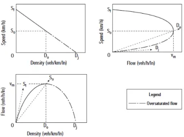
Figure 1. Fundamental diagrams of speed-flow-density relationship (HCM, 2000).
The static approach also referred to a conventional method is based on the relationship
between the three variables of traffic stream namely traffic volume (q), space mean speed (u), and
density (k) as known as the fundamental diagram. One of the advantages of this approach is that
it is not necessary to acquire data at a bottleneck. One must observe traffic at different volumes to make a reliable curve fitting possible. If the observed traffic state in unstable or even worse (congested), the result of the curve fitting state depend too much on the type of curve chosen because of the great variance in these observed values. A major disadvantage of the fundamental
diagram is requirement of mathematical model that fits the observed data pairs. Minderhoud et al.
(1997) noted that in order to satisfy this model, it is necessary to collect sufficient data over a broad range of intensities to make a reliable curve fitting possible.
Further, a fundamental diagram is used for determining capacity on the highway in the HCM 2000 guideline based on the relationship speed-flow diagram. The volume at the apex of the speed-flow diagram is determined by applying the speed-flow-density relationship (May, 1990); Van Aerde and Rakha (1995). The relationship among traffic flow and density of the road segment is illustrated within the fundamental diagram. For example, Figure 1 illustrates that two speed values belonging to two traffic flow conditions, one for uncongested traffic and another for congested condition. Additionally, Van Aerde and Rakha (1995) proposed a single regime car following model. This approach is based on the minimum desired distance headway between
67
consecutive vehicles as the sum of constant terms, a term depending on the difference between the current speed and the free speed, and term depending on the current speed. The speed-density relationship is given by:
(1)
where d represents traffic density (veh/h), v represent space mean speed (km/h), ∆x is distance
headway between consecutive vehicle (km), v0is free flow speed (km/h), andc1,c2,c3 are unknown
parameters in which can be calibrated by using non-linear regression.
Selected Maxima (or Expected Value)
A common approach proposed by Minderhoud et al. (1997)based on the selected maxima
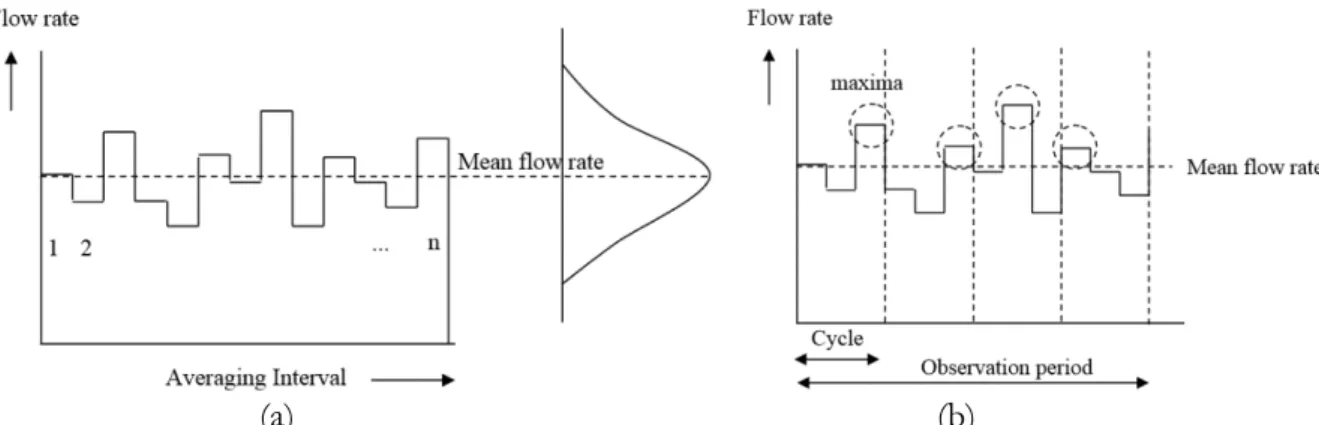
principle uses maximum flow rates measured over the observation period. The capacity of the road assumes that to be equal to the selected flow maxima distribution observed during the period of observation. In its original method, traffic flow that observed within intervals less than an hour is used. Then, the capacity is defined as supposed to be an equal to the average maximum traffic
flow during observation as given by , where qc represents capacity value (veh/h), qi
represents maximum flow rate observed over period, N is number of cycles and i is observation
cycles. Noted that Minderhoud et al. (1997) suggested taking capacity value by 90th percentile is
might useful for minimizing the variation thereby increasing the reliability of the calculated
capacity value. In addition of maxima method, Hyde et al.(1986) and Minderhoud et al. (1997) used
direct probability (expected extreme value) method. They proposed direct probability method may be applied when the capacity of the road has been reached. The capacity estimating resulting from the calculations can be considered as a certain exceptional value of the maximum flow. Thus, the capacity of the road is based on the expected maximum flow rate predicted the distribution of traffic counts given assumed traffic arrival process. Moreover, the asymptotic method is another
approach to solving the extreme value estimation problem proposed by Hyde et al. (1986). The
method relies on the theory that behavior of extreme value arising from any natural process can be described in terms of a simple statistical model.
The capacity is calculated as the expected maximum flow rate predicted from the distribution of observed extremes in selected intervals. Disadvantage of the asymptotic method is more practical approach due to lack of theoretical background. It is also because of selecting capacity depends on the duration of averaging interval, it appears that the expected maximum more practical method rather than theoretical sound. The main reason is great variance in capacity values observed because this method mostly considers to high traffic volumes in determining capacity rather than low traffic volume. In other words, the selected maxima method is more appropriate compared with the expected extreme value method particularly for asymptotic method. The difference among two expected value methods including direct probability and asymptotic approaches can be seen in Figure 2.
68
(a) (b)
Figure 2.Comparison of (a) direct probability and (b) asymptotic method
Dynamic Approaches
Dynamic highway capacity estimation (DHCE)
Dynamic highway capacity estimation (DHCE) relies on statically distributions of observed
traffic flow. This method is formerly proposed by Chang and Kim (2000) and Zunhwan et al. (2005).
They developed a method for presenting alternative a quantitative method for highway capacity by evaluating alternative approaches in developing capacity from statically distributions of observed of traffic flow. The works were shown that extremely long headways are considered to be unreasonable (subjected to outliers) to sufficient demand and for the maximum flow rate defining. Therefore, the longer headways are removed from measured data. To determine the threshold which defines as long headways confidence intervals of 90%, 95%, and 99% from headway distribution has been used. Further, cumulative distribution of volumes was evaluated at their 85, 90, and 95 percentiles. Then the composite valuation of headways corrected by the long headway and volume distribution percentiles is performed. Highway capacity can be described as the ability of roadway in response to drivers and vehicles. The ability of the roadway is revealed as a vehicle’s speed and time headway. A roadway capacity is a function of the driver’s and vehicle’s condition, vehicles speed and headway, as defined in equation below:
Ci= f (D,V,S,H) (2)
Where C represents a capacity of roadway i, V is vehicle condition, H represents time headway
(second), D is driver condition, and S is speed of vehicles (km/h). By considering the unit of time
in hour, Equation (2) can be reformulated as:
(3)
Assuming that the driver condition and vehicle condition follow a certain distribution and set
as error term, Equation (3) can be restated as Hci = g’ (S) +
ε
, with Hci is time headway at Ci andε
is random error component. Time headway at capacity Ci can be estimated and then various
capacities changed by speed Cs are calculated as Cs = 3600/Hci. From above derivation, it clearly
shows that the concept of dynamic capacity of the highway capacity method, which can vary with the speed of vehicles. The DHCE algorithm is then as follows: 1). Data collection for disaggregated data individual vehicle's time headway and speed. 2). The process of rejection abnormal data and select capacity data using capacity index. 3). Process for estimating coefficients of DHCE model using filtered data. The headway distribution model equation such as polynomial, linear and exponential at each capacity index 85%, 90 % and 95%, and the
69
polynomial model chosen as the best model with respect to higher R2. 4). Process of identifying
dynamic capacity using DHCE model.
Breakdown Probability Function
By the definition and understanding of the roadway capacity is a notation that the facility becomes congested and breakdown. Elefteriadou and Lertworawanich (2003) defined breakdown as a traffic stream condition in which transition from non-congested (stable) state to a congested state (unstable) when demand exceed the certain capacity values. Moreover, Lertworawanich and Elefteriadou (2001)mentioned that breakdown does not necessarily occur always in the same demand levels, but can occur when flow are lower or higher than the numerical value traditionally accepted as capacity. Breakdown could probably occur at flows lower than the maximum
observed, or capacity flows (Elefteriadou et al., 1995).The term of breakdown describes highway
operation near the bottleneck entrance during a period when there is a change of operation with
vehicle flowing freely to operation with queue present (Persaud et al., 1998). It is the attractive
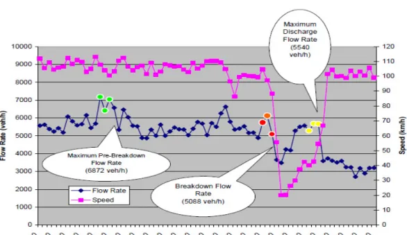
possibility of increasing flow and speed by preventing breakdown in congestion operation. This possibility has been fueled by observation of a capacity drop where in the discharge flow from the resulting queue is smaller than those observed before breakdown. Additionally, Zhang (2001) proposed three kinds of capacity when a breakdown occurs in particular roadway section. One is for acceleration flow; others are deceleration flow and stationary flow. Ideal capacity could be adopted from the stationary flow as operation capacity. Breakdown probability function for quantifying three capacities on the active bottleneck based on time series plots of flow and speed. According to Lorenz and Elefteriadou (2001) and Elefteriadou and Lertworawanich (2003) the steps of analyzing as follows:1). Identify and quantify each transition interval from non-congested to congested flow, breakdown event, and document the corresponding breakdown flow. Identified and defined breakdown as a speed drop at a certain level and breakdown capacity defined immediately before breakdown occurs. In this research, the breakdown flow is defined as the 5-minutes flow (for 5-min aggregation intervals) or 15-minute flow (for 15-minutes aggregation intervals) immediately prior to the breakdown. 2). Identify and document the maximum pre-breakdown flow. This flow is the maximum observed at the site prior to the occurrence of congestion. As for breakdown flow analysis, both 5-minute and 15-minute aggregation intervals were suggested. 3). Identify and document the maximum discharge flow. This flow is the maximum observed at the site after the occurrence of breakdown, and prior to recovery to non-congested conditions.
Figure 3 illustrates these three variables in a single time-series plot correspondent to capacity identifying when pre-breakdown, breakdown and maximum discharge flow. Figure 4 shows the
capacity drop and capacity in queue discharge flow as suggested by Brilon et al. (2007) capacity can
directly measure in queue discharge flow immediately before recovery of traffic flow. Statistical analyses were conducted to evaluate the distributions obtained, and to compare their parameters.
The χ2is suggested to compare these distributions to the normal distribution. It was concluded
that all distributions fit the normal at the 5% level of significance. The t-test was used to compare the mean values of each of the flow rates.
70
Figure 3.Three breakdown capacity in time-series plot of flow and speed (Elefteriadou and Lertworawanich, 2003)
Figure 4. Flow rate and speed time series during congested
71
(a)
(b) (c)
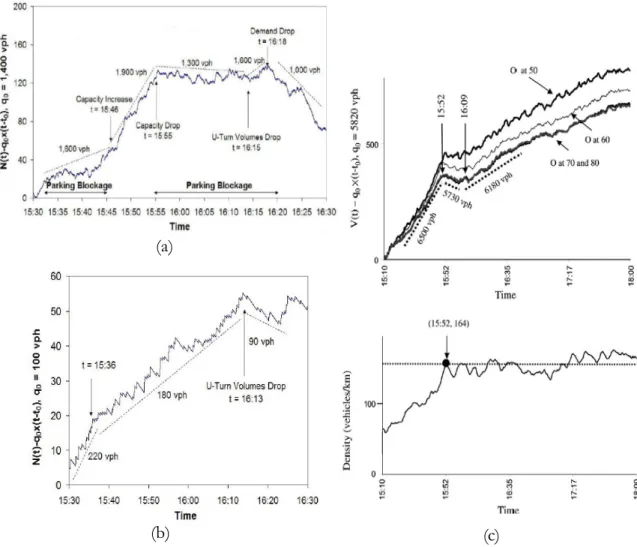
Figure 5. Oblique cumulative plots and capacity drops. (a) Capacity drop by parking blockage, (b) Capacity drop by U-turn, (c) Capacity drop and density drop
(Rudjanakanoknad, 2009)
Oblique Cumulative Plot (O-Curve)
Analyzing roadway capacity based on dynamic behavior on bottleneck section using oblique cumulative plots was formerly proposed by Cassidy and Windower (1995). This method is a special time-series data treatment that could illustrate the change in driver behavior and use to analyze the effect of activities that contribute to change in street capacity. This technique has been generally used in numbers
of traffic dynamic researches (Cassidy and Bertini, 1999), Cassidy and Rudjanakanoknad (2005), Chung et
al. (2007)). However, these works mostly were done on uninterrupted-flow-facility or freeway traffic only,
the attempt of using this technique on an interrupted flow facility such as a local street has not yet been widely applied. The first work was done in the arterial road in Bangkok, Thailand by Rudjanakanoknad
(2009) and carried out in Banda Aceh, Indonesia by Sugiarto (2012), Sugiarto et al. (2012; 2013). These
works deal with assessing the capacity and travel speed drop in arterial road and identify the factor that effect with the capacity drop during virtual bottleneck occurs. Two factors were identified namely blocked area by median opening section and on street parking space during afternoon peak hours. The oblique cumulative plot technique such that traffic mechanism at the site can be examined by visualizing the changes in flow rates from each different measurement and comparing across observation days. The
72
analysis results show the degrees of how these individual factors affect the street bottleneck capacity due to median opening and on street parking activities.
The methodology of oblique cumulative plots (O-Curve) is based on a cumulative vehicle arrival number to time arrival. The cumulative arrival curve is a visual presentation of observations collected directly from the roadway segment. The measurement flow requires a short time period such as one minute or even less, and the time interval selected can be influence the magnitude of the flow. Oblique
cumulative plots is a special time-series data treatment O(t) versus t, with mathematically is given by O(t)
= N(t) - qo(t-to). Where O(t) represents a cumulative vehicle after re-scaled, N(t) represents a
cumulative vehicles count during time t, qo is selected background flow and to is starting time, to=0.
Oblique cumulative plots is shown magnitude of the traffic flow by the time and amplifies change is slope. The slope of the oblique cumulative plots must be proportional to the flows of measurement. Thus, the plot of the slope is facilitated visual identification of the time when these flows actually changed, as for the illustration can be seen in Figure 5a and Figure 5b. Moreover, the relation between vehicle density and losses in discharge flow is illustrated in Figure 5c. Chung
et al. (2007) work was done for analysis relationship between capacity drop and density. Each bottleneck suffered reductions in discharge once queues formed just upstream. This so-called capacity drop was related to the density measured over some extended-length freeway segment near each bottleneck.
Product Limit Method (PLM)
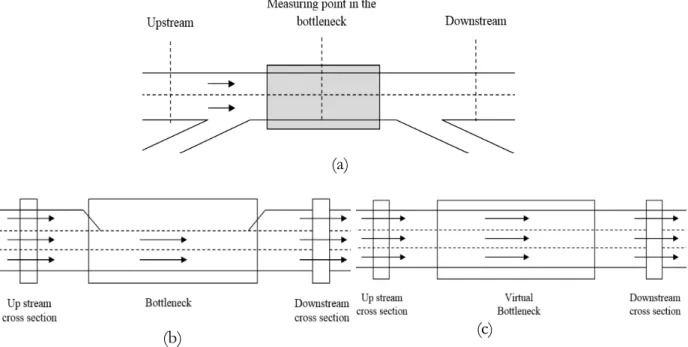
The theory behind the product limit method is based on explicit division of traffic flow observations. It can easily be understood that a flow rate measurement at a cross section in Figure 6 can be divided into one of two categories if the upstream traffic state is observed: measurement representing traffic demand (a free flow intensity measurement) and measurement representing the capacity state of the road (upstream congestion). This category of observation is an important aspect of the product limit method.
This method allows estimation of capacity distribution function F(q) with both free-flow intensities and
capacity observations.
(a)
(b) (c)
Figure 6.Measuring point at a bottleneck and two types of roadway bottleneck; (a) Measuring
point at a bottleneck, (b) Systematic bottleneck, (c) Unsystematic bottleneck (virtual)
73
Due to reliability analysis, this method requires more than single day volume and speed measurements. Moreover, a bottleneck location should be chosen to be sure about the capacity state of road whenever congestion in detected upstream. The product limit method (PLM) is a useful solution for estimating the capacity distribution function of a roadway from traffic observations. For practical application, two items remain to be defined: 1). Duration of observation intervals, for analysis, only rather short observation intervals are useful. Otherwise the causal relationship between traffic volume and breakdown would be too weak. 1-hour counts, for example, are not adequate for this reason. Ideally the observation period should be 1 minute or
even less (Brilon et al., 2007), after experiments with different ∆t, came to the conclusion that ∆t = 5
minutes were the best compromise. 2). Understanding of a breakdown, the definition of a breakdown
mentioned PLM formula is a decisive aspect of the whole methodology. As defined by Minderhoud et al.
(1997) that breakdown capacity as the volume measured downstream of a queue at a bottleneck. Consequently, each congested flow volume is regarded as a B-value. As a breakdown of traffic flow usually involves a significant speed reduction, breakdown events can be detected using a time series containing both traffic volumes and average space mean speeds. This is done by using a constant threshold speed value. The capacity of a roadway section can be analyzed most precisely if observations are made at a clearly distinguishable bottleneck as shown in Figure 6. At such a bottleneck, breakdowns should only be caused by oversaturation of the bottleneck itself. A tailback from downstream should not occur as greater capacities are always available in the succeeding section. Observations are therefore made at a point slightly upstream of the bottleneck.
The practical estimation of product limit method was explained more by Minderhoud et al. (1997).
The derivation is given of simplified approaches in estimating road capacity with traffic volume and speed data with only capacity observation available. This ideal situation leads to so called empirical distribution function of capacity as given:
Fc(q) = P(c≤q) (4)
Where Fc(q) represents capacity distribution function, c iscapacity and q is traffic volume. This
method is used based on analogy to the statistics life data analysis which describes the statistical properties of duration of human life. It is usually applied to analyze the durability of technical component, with the life time distribution function is:
F(t) = 1-S(t) (5)
Where F(t) represents distribution function of life time = p(T≤t), Tis time and S(t) is survival
function = p(T>t). Consequently, the lifetimes of several individuals in the sample exceed the
duration of the experiment and therefore cannot be measured. It is only possible to state that these lifetimes are longer than the duration of the experiment. If a traffic breakdown is regarded as a failure event, the methods for lifetime data analysis can be used to estimate the capacity c,
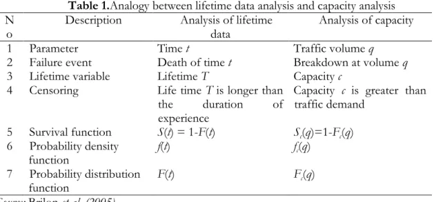
which is the analog of the lifetime T. The parameter analogy between capacity analysis and lifetime
data analysis is given in Table 1.The statistics of life time data analysis can be used to estimate distribution functions based on samples that include censored data. A non-parametric method to estimate the survival function is of PLM proposed by Kaplan and Meier (1958) is used.
74
where represents estimated survival function, nj is number of individuals with a lifetime T≥t, and dj
is number of death as time tj, tj value equal 1 (censored data). Empirical capacity distribution
functions for specific roadway, traffic, and control conditions can be estimated by using mathematical methods for lifetime data analysis. The capacity, whose distribution function represents the probability of a traffic breakdown during a particular time interval, is considered as a lifetime variable. In this analogy, the breakdown of traffic flow represents the failure event.
Table 1.Analogy between lifetime data analysis and capacity analysis N
o
Description Analysis of lifetime
data
Analysis of capacity
1 Parameter Time t Traffic volume q
2 Failure event Death of time t Breakdown at volume q
3 Lifetime variable Lifetime T Capacity c
4 Censoring Life time T is longer than
the duration of
experience
Capacity c is greater than
traffic demand 5 Survival function S(t) = 1-F(t) Sc(q)=1-Fc(q) 6 Probability density function f(t) fc(q) 7 Probability distribution function F(t) Fc(q)
Source: Brilon et al. (2005)
Traffic flow observations on roadways deliver pairs of values of flow rates and average speeds in particular time intervals (Geistefeldt, 2008). For capacity analysis uncensored and
censured intervals are distinguished. An interval i is classified as uncensored if the observed flow
rate qi causes a breakdown of traffic flow, thus the average speed drops below a specific threshold
in the next interval i+1. In this case, the flow rate qi is regarded as a realization of the capacity c. If
traffic is fluent in interval i and remains fluent in the following interval i+1, this observation is
classified as censored, which means that the capacity c in interval i is greater than the observed
flow rate qi. Intervals after breakdown with an average speed below the threshold are not
considered for analysis because volumes observed under congested flow conditions do not contain any information about the capacity in fluent traffic. To estimate distribution functions based on samples that include censored data, both non parametric and parametric. The non-parametric PLM can be drawn by restated from Equation (5) combined with Equation (6) as follows:
Fc (q) ; i∈{B}
(7)
where Fc(q) represents distribution function of capacity c, q is traffic volume, qi is traffic volume in
interval i, ki is number of intervals with traffic volume of q≥qi, di is number of breakdowns at
volume of qi, and {B}is set breakdown interval if traffic is fluent in interval i, but the observed
volume causes a breakdown (i.e. the average speed drop below the threshold speed in the next interval i+1). The distribution function will only reach a value of 1 if the maximum observed volume is an uncensored value such as followed by a traffic breakdown. Otherwise, the
distribution function terminates at value of Fc(q)<1. For a parametric estimation, the function
type of the distribution must be predetermined. The distribution parameters can be estimated by applying the Maximum Likelihood Estimation (MLE) method. For capacity analysis, the Likelihood function is given:
75
(8)
Where fc(qi) represents statistical density function of capacity, Fc(qi) is cumulative density function
of capacity, n is number of interval,
δ
i is 1, if uncensored (breakdown of classification B),δ
i is 0,otherwise. There were various plausible function types such as Weibull, Normal and Gamma distribution can be tested. An empirical comparison between different function types revealed that
freeway capacity is Weibull distributed (Brilon et al., 2005). The Weibull type capacity distribution
function is given by:
(9)
Where fc(qi) represents capacity distribution function, q is flow rate (veh/h),
α
is shape parameterand
β
is scale parameter (veh/h). The shape parameterα
determines the variance of thedistribution function. The variance decreases with increasing shape parameter. The scale
parameter
β
is proportional to both the mean value and the standard deviation of the distributionfunction. The scale parameter represents the systematic factors affecting freeway capacity, such as number of lanes, grade, and driver population (Geistefeldt, 2008).
Table 2. Summarize of the Capacity Estimation Methods.
No Methods Required data Result of analysis
1 Conventional Method (IHCM,
1997; HCM , 2000)
Speed and flow rate
Single constant value of capacity
2 Selected maxima method
(Minderhoud et al. 1997)
Flow rate and time Maximum capacity and 90th percentile of capacity.
3 Dynamic highway capacity
estimation method (Chang and Kim
(2000);Zunhwan et al. (2005))
Speed and headway
Headway-speed relationship. Capacity distribution in every expected speed
4 Breakdown probability function
method (Elefteriadou et al. (1995);
Elefteriadou et al. (2003); Persaudet
al. (1998); Zhang, (2001);
Lertworawanich and Elefteriadou
(2001); Sugiarto (2012); Sugiarto et
al. (2012); Sugiarto et al. (2013)).
Flow rate, speed and Time of arrival Pre-breakdown capacity Breakdown capacity Discharge capacity Speed threshold of a breakdown
Time threshold of breakdown
5 Oblique cumulative plots, (Cassidy
and Windower (1995); Cassidy and Bertini (1999); Cassidy and
Rudjanakodnad (2005); Chung et al. (2007); Rudjanakodnad, (2009); Sugiarto (2012); Sugiarto et al. (2012; 2013)) Vehicle arrival, time of vehicle arrival Pre-breakdown capacity Breakdown capacity Discharge capacity
Time threshold of breakdown Capacity drop
Density drop.
6 Product limit method (Minderhoud
et al. (1997); (1986); Brilon et al.
(2007); Geistefeltd (2008); Brilon et
al. (2005)).
76
Conclusions
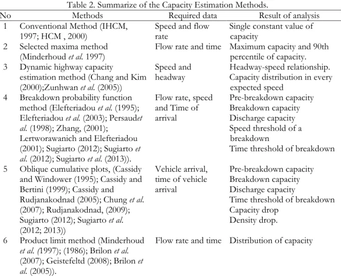
By comparing the conventional method of IHCM (1997) and relevant existing methodologies (i.e. static, dynamic), it seems that the dynamic approach is more suitable for analyzing traffic breakdown in bottleneck including capacity and speed dropped. We summarize existing methodologies including proposed methods, required data and expected results as described in Table 2. Respecting the static method, it does not appropriate for detecting and visualizing traffic breakdown mechanism in bottleneck traffic situations due to does not systematically take into account of bottleneck activities. Implementation of this method is likely more easy and practical oriented compare to dynamic approach. However, noted that capacity prediction based on physical suggested in HCM can be misleading. On the other hand, the advantages of dynamic method (i.e. oblique cumulative plots, breakdown probability function) are powerful in identifying the fluctuation of traffic flow and better visualizing even only by plotting time-series treatment from traffic data such as time, vehicles arrival and speed. However, the drawback of this method is very time consuming in terms of data processing but using current advance technologies such as loop detector could overcome this problem. This paper carefully summarize the merit of existing methodologies, we further notice that dynamic approaches could be more appropriated for analyzing temporal congestion segments (median opening, on street parking, etc.). Method of oblique cumulative plot seem to be more applicable in terms of convenient, surveying tool and the accuracy of analysis. This method is easy to handle and powerful in identifying the fluctuation of flow and speed during breakdown occurs.
References
Brilon, W., Geistefelt, J., and Regler, M. 2005. Reliability of freeway traffic flow: A stochastic concept of capacity. Proceeding of the 16th International Symposium on Transportation and Traffic Theory, 125-144, College park, Maryland, July 2005.
Brilon, W., Geistefeldt, J., and Zurlinden, H. 2007. Implementing the concept of reliability for highway capacity analysis. Journal of Transportation Research Record, 2027: 1-8.
Cassidy, M.J., and Windover, J.R. 1995. Methodology for assessing dynamics of freeway traffic flow. Transportation Research Record, 1484: 73-79.
Cassidy, M.J., and Bertini, R.L. 1999. Some traffic features at freeway bottlenecks. Transportation Research Part B, 33: 25-42.
Cassidy, M.J., and Rudjanakanoknad, J. 2005. Increasing the capacity of an isolated merge by metering its on-ramp. Transportation Research Part B, 39: 896-913.
Chang, M. and Kim, Y. 2000. Development of capacity estimation method from statistical distribution of observed traffic flow. Proceedings 4th International Symposium on Highway Capacity, 299-309.
Chung, K., Rudjanakanoknad, J. and Cassidy, M.J. 2007. Relationship between traffic density and capacity drops at three freeway bottlenecks. Transportation Research Part B, 41: 82-95. Elefteradou, L. and Lertworawanich, P. 2003. Defining, measuring and estimating freeway
capacity. The 82nd Annual Meeting of Transportation Research Board, Washington, DC, USA, January 12-16.
Elefteradou, L., Roess, R.P. and McShane, W.R. 1995. Probabilistic nature of breakdown at freeway merge junctions. Journal of Transportation Research Record, 1484: 80-89.
Geistefeldt, J. 2008. Empirical relationship between stochastic capacities and capacities obtained from the speed-flow diagram. Symposium on the fundamental diagram: 75 years, Monograph 01109339. Woods Hole, Massachusetts, July 8-10.
Hyde, T. and Wright, C. 1986. Extreme value methods for estimating road traffic capacity. Transportation Research Part B, 20(2): 125-138.
77
Kaplan, E.L. and Meier, P. 1958. Nonparametric estimation from incomplete observations. Journal of the American Statistical Association, 53: 457-481.
Lertworawanich P. and Elefteriadou, L. 2001. Capacity estimations for type B weaving areas based on gap acceptance. Journal of Transportation Research Record, 1776: 24-34.
May, A.D. 1990. Traffic flow fundamentals. Willey and Soon, London.
Minderhoud, M.M., Botma, M. and Bovy, P.H.L. 1997. Assessment of roadway capacity estimation methods. Journal of the Transportation Research Record, 1572: 59-67.
Persaud, B., Yagar, S. and Brownlee, R. 1998. Exploration of the breakdown phenomenon in freeway traffic. Journal of Transportation Research Record, 1634: 64-69.
Rudjanakanoknad, J. 2009. Analysis of effecting street bottleneck capacity through oblique cummulative plots. Proceeding of the Eastern Asia Society for Transportation Study, Surabaya, Indonesia.
Sugiarto. 2012. Traffic breakdown mechanism of hidden bottleneck: A case study of U-turn section on an arterial road. Jurnal Teknik Sipil, 1: 67-76.
Sugiarto, Limanond, T. and Nakatsuji, T. 2012. Dropped in capacity and traffic speed of urban Arterial: a case study at u-turn section in Aceh Province, Indonesia. Aceh International Journal of Science and Technology, 1(3): 86-92.
Sugiarto, S., Limanond, T. 2013. Impact of on-street parking on urban arterial performance: A quantitative study on travel speed and capacity deterioration. Aceh International Journal of Science and Technology, 2(1): 63-69.
HCM. 1985. Highway capacity manual 1985. Transportation Research Board, Washington D.C. HCM. 2000. Highway capacity manual 2000. Transportation Research Board, Washington D.C. Van Aerde, M. and Rakha, H. 1995. Multivariate calibration of single speed-flow-density
relationship. In Proceedings of the 6th 1995 Vehicle Navigation and Information Systems Conference (1995), pp. 334–341
Zhang, H.M. 2001. A note on highway capacity. Transportation Research Part B, 35: 929-937. Zunhwan, H., Jumsan, K. and Sungmo, R. 2005. Development of a new highway capacity
estimation method, Proceedings of the Eastern Asia Society for Transportation Studies, 5: 984-995.