Mobile Network Data Analytics for Intelligent Transportation Systems

(1)

PhD-FSTC-2018-14

The Faculty of Sciences, Technology and Communication

DISSERTATION

Defence held on 07/02/2018 in Luxembourg

to obtain the degree of

DOCTEUR DE L’UNIVERSITÉ DU LUXEMBOURG

EN INFORMATIQUE

by

Thierry

DERRMANN

Born on 24 June 1987 in Dudelange (Luxembourg)

MOBILE NETWORK DATA ANALYTICS

FOR INTELLIGENT TRANSPORTATION

SYSTEMS

Dissertation defence committee

Prof. Dr. Thomas Engel

,

dissertation supervisor

Professor, University of Luxembourg

Dr. Raphaël Frank

Research Scientist, University of Luxembourg

A-Prof. Dr. Francesco Viti, Chairman

Associate professor, University of Luxembourg

Dr. Marco Fiore

Researcher, National Research Council of Italy

Prof. Dr. Falko Dressler,

Vice Chairman

(2)

(3)

Acknowledgements

This work was conducted at the SECAN-Lab of the University of Luxembourg’s Inter-disciplinary Centre for Security Reliability and Trust (SnT). The project was funded by the Luxembourg Fonds National de la Recherche (FNR).

First and foremost, I would like to thank Prof. Dr. Thomas Engel for letting me conduct my research at SECAN-Lab, allowing me to freely explore, identify and investigate my topics of interest, while always being supportive.

I would also like to thank Dr. Rapha¨el Frank for his continuous advice, motivation, and the much-needed criticism of my work, but also for showing me around campus at UCLA.

I also want to thank Prof. Dr. Falko Dressler for taking the time to supervise my progress and for the excellent work done by him and his team at the University of Pader-born, especially Dr. Christoph Sommer and Florian Hagenauer, co-creators of Veins and VeinsLTE. Without their works, this dissertation would not have been possible.

Further, I want to thank Prof. Dr. Francesco Viti, who supported me in my ven-ture into the field of transportation, giving me invaluable pointers to the right models and literature, especially in traffic flow theory, and opportunities for joint publications at transportation conferences. I also want to thank his MobiLab team members Guido Cantelmo and Dr. Marco Rinaldi for their help with the transportation-related topics in this thesis.

Finally, I would like to thank all my colleagues at SECAN-Lab, MobiLab and at SnT who made work and conferences so much more enjoyable. Most of all, I want to thank my family and friends, who have always been supportive of my efforts and understanding when things were not going as planned.

(4)

(5)

Abstract

In this dissertation, we explore how the interplay between transportation and mobile networks manifests itself in mobile network billing and signaling data, and we show how to use this data to estimate different transportation supply and demand models.

To perform the necessary simulation studies for this dissertation, we present a simula-tion scenario of Luxembourg, which allows the simulasimula-tion of vehicular Long-Term Evolu-tion (LTE) connectivity with realistic mobility.

We first focus on modeling travel time from Cell Dwell Time (CDT), and show – on a synthetic data set– that we can achieve a prediction Mean Absolute Percentage Error (MAPE) below 12%. We also encounter proportionality between the square of the mean CDT and the number of handovers in the system, which we confirmed in the aforementioned simulation scenario. This motivated our later studies of traffic state models generated from mobile network data.

We also consider mobile network data for supporting synthetic population generation and demand estimation. In a study on Call Detail Records (CDR) data from Senegal, we estimate CDT distributions to allow generating the duration of user activities, and validate them at a large scale against a data set from China. In a different study, we show how mobile network signaling data can be used for initializing the seed Origin-Destination (O-D) matrix in demand estimation schemes, and show that it increases the rate of convergence.

Finally, we address the traffic state estimation problem, by showing how handovers can be used as a proxy metric for flows in the underlying urban road network. Using a traffic flow theory model, we show that clusters of mobile network cells behave characteristically, and with this model we reach a MAPE of 11.1% with respect to floating-car data as ground truth. The presented model can be used in regions without traffic counting infrastructure, or complement existing traffic state estimation systems.

(6)

(7)

Acronyms

AP Access Point.

ATIS Advanced Traveller Information System.

BC Bluetooth Classic.

BLE Bluetooth Low Energy.

C-ITS Cooperative Intelligent Transportation Systems.

CDR Call Detail Records.

CDT Cell Dwell Time.

CGF Charging Gateway Function.

DARC Data Radio Channel.

DSRC Dedicated Short Range Communications.

FCD Floating-Car Data.

FD Fundamental Diagram of Traffic Flow.

GGSN Gateway GPRS Support Node.

GMSC Gateway Mobile Switching Center.

GPS Global Positioning System.

(10)

GTFS General Transit Feed Specification.

GTFS-RT General Transit Feed Specification: Real-Time.

ICT Information and Communication Technology.

IMEI International Mobile Equipment Identifier.

IMSI International Mobile Subscriber Identifier.

ITS Intelligent Transportation System.

LTE Long-Term Evolution.

LWR Lighthill-Whitham-Richards model.

MAC Medium Access Control.

MAPE Mean Absolute Percentage Error.

MFD Macroscopic Fundamental Diagram.

MIMO Multiple-Input and Multiple-Output.

MME Mobility Management Entity.

MNO Mobile Network Operator.

MSC Mobile Switching Center.

NFD Network Fundamental Diagram.

O-D Origin-Destination.

PDN-GW Packet Data Network Gateway.

RAN Radio Access Network.

RNC Radio Network Controller.

(11)

Acronyms ix

RSU Road-Side Unit.

S-GW Serving Gateway.

SGSN Serving GPRS Support Node.

SNR Signal-to-Noise Ratio.

SSID Service Set Identifier.

TDM Transportation Demand Management.

TETRA Terrestrial Trunked Radio.

TIS Traffic Information System.

UMTS Universal Mobile Telecommunications System.

V2I Vehicle-to-Infrastructure Communication.

V2V Vehicle-to-Vehicle Communication.

V2X Vehicle-to-Everything Communication.

VANET Vehicular Ad Hoc Network.

(12)

(13)

Chapter 1

Introduction

”Information is the oil of the 21st century, and analytics is the combustion engine.”

Peter Sondergaard

The ubiquity of mobile phones today is producing ever-increasing amounts of data, providing invaluable information that can be used to study many aspects of our everyday life. According to estimates, there were approximately 7.5 billion mobile subscriptions in 2016, with approximately 7 billion people living within areas with mobile network coverage [1]. Of these 7.5 billion subscribers, 4.5 billion are estimated to be unique users. Figure 1.1 shows the trend of subscribers, world population and population in coverage range of mobile networks. According to the 2017 Cisco Visual Networking Index [2], mobile data traffic has grown 18-fold over the past five years, and with mobile network coverage approaching 100% of the world population, there are increasing efforts to draw benefits from the data that the networks generate.

As the data is generated by large parts of the population, it is representative of many phenomena in our daily lives, and mobile network operators (MNOs) can create new rev-enue streams and aid developing countries [3]. In this vein, MNOs have recently launched research challenges, providing access to large data sets in an effort to extract knowledge therefrom for the benefit of various application domains [4, 5]. An extensive survey on the results in different fields – many of which are based on these research challenges – is provided by Naboulsi et al. [6], showing the vast scope of analyses that mobile data can support, ranging from social studies (e.g. demographics, land use and epidemiology) to

(14)

Figure 1.1: Evolution of global access to mobile network connectivity [1]

mobility and performance of the mobile network itself. Examples include techniques to facilitate urban planning [7], improve transportation networks [8, 9] and provide insights into the epidemiology of diseases [10].

In another survey on the analysis of mobile network data sets, Calabrese et al. [11] identify numerous topics of interest and open challenges. A common topic of interest between both surveys is the modelling of human mobility patterns, such as the use of mobile network data as a complementary source for estimating dynamic road traffic con-ditions. As a particular open challenge, they mention the characterization of the interplay between mobile networks and the actual mobility of users, while taking privacy and data anonymity considerations into account. Naboulsi et al. confirm that this is especially challenging for urban mobility, as it is much more heterogeneous in infrastructure and user behaviour than highway networks [6].

A major motivation for estimating urban mobility from mobile data is that trans-portation sensing infrastructure is costly in terms of installation and maintenance, has limited coverage and is intrusive. Thus, it is helpful to consider using mobile networks as a distributed sensor network for gathering data on mobility. In a mobile network, all participants generate data, i.e. stationary and mobile users alike. From a transportation

(15)

Introduction 3 perspective, mobile network data can then be referred to as exogenic data, as the data encompasses not just the transportation network agents but the entire userbase around it. This is in contrast toendogenic data generated purely within a transportation system, e.g. via Vehicle-to-Infrastructure Communication (V2I), and providing signals from cer-tain types of users, such as cars or pedestrians exclusively. The main difference between the two approaches thus lies in the way the data is collected: exogenic data is passively generated, while endogenic data is purposefully, actively generated by a specific subset of users.

As the discussion on the most appropriate communication technology for vehicular communication is still ongoing [12], it makes sense to look at the passively collected exo-genic data from mobile networks instead. In this context, and in order to leverage mobile networks and the data generated by its userstoday, it is necessary to study various types of mobile network data and their utility in estimating various transportation metrics. The outcome of this is the following research question:

1.1 Research Question

How do mobile and transportation network behaviours correlate and how can we leverage their interplay for transportation applications?

We want to explore how mobile network data can be used for various estimation and modelling tasks in transportation. Essentially, by looking at mobile networks as distributed traffic sensors, we want to show that they can serve as a complement to the existing, traditional transportation data sources. The aim is to use mobile network data directly, in contrast to data from connected car communication, as the latter is still sparse due to low equipment rates and the ongoing technology dispute. Thus, in the currently ongoing transition phase, exploiting exogenic communication data can provide significant knowledge.

Two main aspects of this research question must be considered.

On one hand, when characterizing the links between the behaviours of transportation networks in relation to that of the mobile network, it is important to measure the impact of stationary users. The question is whether data concerning the full mobile network userbase can be useful for describing only the mobile users, or whether the bias introduced by stationary users is too high. For certain types of data, e.g. regarding connection handovers,

(16)

stationary users may be negligible in comparison to moving users, but the error must be quantified and is likely much higher for other types of mobile data.

On the other hand, it is necessary to investigate which estimation techniques are pos-sible using different types of mobile network data. These types of data can be extracted from the billing system, e.g. CDR, and the core Radio Access Network (RAN), i.e. signal-ing data, and have different uses when it comes to transportation applications. The main applications with respect to private transportation supply are travel time and traffic state estimation. While these metrics are related, travel time estimation is usually concerned only with predicting delays and finding the fastest route, while traffic state estimation refers to the estimation of flow, density and velocity on a road (sub-)network. These metrics are useful for traffic engineering and control, and are key inputs for any Intel-ligent Transportation System (ITS). Demand estimation, on the other hand, typically involves all available modes of transportation, and is most frequently delivered as a set of dynamic O-D matrices that contain the need for transportation between different zones. Demand estimation is relevant for transportation optimization and planning, and is the key component for realistic simulation of transportation systems as well.

We want to explore ways of estimating supply- and demand-related metrics in a cost-neutral and privacy-friendly way. Mobile networks, when used as distributed traffic sensors, are one way of achieving this aim. Thus, we will present mobile network data-based models, in order to show how the main transportation metrics can be estimated. Mobile networks can then be used either alone or jointly with additional data sources to provide accurate estimates of transportation metrics, in rural and urban areas alike.

This research question is of particular interest for applications in areas with little transportation information infrastructure, e.g. in remote areas or in developing countries. For example, according to the 2017 Cisco Visual Networking Index [2], mobile data traffic has almost doubled in 2016 in the Middle East and Africa, a cumulative annual growth rate of 65% is forecast for the coming five years. Combined with the current, high coverage rate, as shown in Figure 1.1, we can expect mobile data to become increasingly valuable for knowledge discovery. The mobile network operators’ data challenges and research efforts show that they share this view [4,5]. Thus, the research question has commercial potential, as there is real value to be extracted from mobile data.

In general, exploiting mobile network data is useful for transportation agencies, as it comes at low cost and with high spatial coverage, and it can provide additional insight.

(17)

Introduction 5

1.2 Methodology

We evaluate the utility of mobile data for estimating transportation metrics of supply and demand in both simulated or synthetic, and real data.

First, in Chapter 3, we introduce a simulation package that was created for the purpose of performing studies for this dissertation, in particular for the traffic state estimation in Chapter 6.

Before using real data we performed studies on synthetic and/or simulated data for the main transportation metrics that we considered, i.e. traffic state, travel times and demand. Our studies on traffic states and travel times concern road traffic (private transportation), while we provide methods for demand estimation that can consider public transportation as well.

The types of data that we base our studies on are the following:

❼ Call Detail Records (CDR) – Billing Data

❼ Aggregated Handover Counts – Signalling Data

❼ Floating Car Data (FCD) – Road Traffic Ground Truth

Initially, we worked on CDR data, as it is the most widely adopted type of data in mobile data analysis. We based our first study on CDRs from the 2015 D4D challenge [4], then proceeded to generate synthetic CDT data from Floating-Car Data (FCD) and CDR data for the estimation of travel times and activity duration in demand estimation. The rationale behind this choice is that CDT offers a direct way of modeling the mobility behavior of mobile network users, conditioned on their current and/or previous or next locations.

For road traffic state estimation, we decided to use concepts from traffic flow theory, which rely on aggregated flows. With privacy concerns in mind, we opted for aggregated handover data, which was kindly provided by a Luxembourgish Mobile Network Operator (MNO). The idea behind this choice was to abstract individual user movements and instead consider handovers inside the network to approximate flows.

To summarize, in all our studies, we built models that are privacy-neutral, as they are based on aggregated data, and we synthesized the contained information into fitted model parameters. We demonstrate the utility of the proposed mobile network data-based models in predicting different transportation supply and demand metrics. In the case of traffic state estimation, we also compare real data and simulation results.

(18)

1.3 Contributions

The first contribution consists of a simulation scenario of Luxembourg City with LTE mobile network infrastructure, which allows jointly simulating cars’ mobility and their connectivity to the LTE network. This contribution is presented in Chapter 3, and was published in [Derrmann et al., 2016a]. The simulation package is freely available online1. The second contribution consists of a study of the adequacy of mobile phone cell dwell times for travel time estimation. Based on synthetic data generated from FCD, we show that distributions of cell dwell times are a promising, privacy-friendly predictor for travel times in an urban setting. This contribution is presented in Chapter 4, and was published in [Derrmann et al., 2016b].

In the third contribution, we show that CDR data can serve as a valuable input for travel demand estimation, in particular the estimation of activity durations. This contribution models the temporal aspect of mobility, while the spatial aspect was handled by Di Donna et al. [13] within the joint MAMBA project framework. This contribution is presented in Chapter 5, where we additionally show how handovers can be used in activity-based demand estimation. This work was published in [Cantelmo et al., 2017].

The final,main contribution of this work is the traffic state estimation model we present in Chapter 6. We introduce a methodology for estimating vehicular density and flows in analogy to the Macroscopic Fundamental Diagram, using mobile network handovers as input data. We show that the presented model works both in simulated- and real-data settings, and compare the results from both worlds. This contribution was published in [Derrmann et al., 2017b, Derrmann et al., 2017a, Derrmann et al., 2017c], and the results were consolidated in a journal article submission that is currently undergoing review.

1.4 Structure

This dissertation is organized as follows. In Chapter 2 we present research related to the topic of using Information and Communication Technology (ICT) data analytics in ITS, introducing the required transportation models and show how different communication networks can be used for fitting transportation models.

In Chapter 3, we present the LuST-LTE simulation package, which produces realistic mobile and road network traces for Luxembourg City, and we perform a preliminary

1

(19)

Introduction 7 validation of its behaviour.

Our first study in Chapter 4 shows how travel time estimation can be performed with mobile network data, yielding some limited, but promising results based on synthetic mobile network signaling data.

In Chapter 5, we show how mobile network data can support demand estimation techniques, and how it can be used for generating synthetic population data.

Chapter 6 presents a novel model linking traffic flow theory and mobile network data, which allows estimating traffic states on a macroscopic scale from mobile network signalling data.

We conclude our work in Chapter 7, summarizing the findings and giving perspectives for future work in this field.

(20)

(21)

Chapter 2

Intelligent Transportation Systems

and Communication Technologies

Intelligent Transportation System (ITS) are defined as transportation systems that rely on Information and Communication Technology (ICT) to leverage information exchange between participants. The purpose of an ITS is the optimization of the performance of a transportation system with respect to specific target attributes such as average travel time or operational cost. This goal is achieved by sourcing sensor input data, evaluating supply and demand models of the transportation network, and using actuators to influence the behaviour of the network and enforce control policies. In the following sections, we provide a non-exhaustive introduction of these models and the data sources which they are based on, as well as the role of communication networks in the improvement of today’s transportation networks.

2.1 Transportation Models

Generally speaking, the models used for transportation systems can be grouped into three distinct groups:

❼ Supply models describe the available capacity – static or dynamic – of a trans-portation mode or (sub-)network in terms of passengers or vehicles with respect to different factors influencing the state of the network.

❼ Demandmodels describe the need for transportation in terms of passengers, freight volume or weight, depending on different environmental and spatio-temporal factors.

(22)

❼ Assignment models allocate demand to the available supply resources.

In this dissertation, we concentrate on supply and demand model parameters from mobile data, which we now introduce in more detail. For a more in-depth insight into this topic, we suggest the books by Sheffi [14], Ortuzar and Willemsen [15] and Cascetta [16].

2.1.1 Demand Models

Demand models allow synthetic representations of the need for transportation in a given network to be created. The two main categories of demand estimation models are thetrip-based and activity-based variations.

Trip-based demand models, the most established of which is the four-step model [17], consider trips independently from each other. The four-step model is defined by the steps of trip generation, distribution, mode choice and network assignment. Trip generation denotes the production and attraction of trips by zones. Trip distribution then allocates trips between pairs of zones, e.g. using the gravity model, yielding an Origin-Destination (O-D) matrix. Finally, mode choice and network assignment distribute the identified demand onto different transportation modes and route alternatives.

Recently, the focus of research has shifted towards behavioural models, i.e. activity-based demand models. They reproduce demand through the mobility needs, as defined by activity sequences. Through the chain of individuals’ locations and the duration of their activities in those locations, the aggregate demand can be extracted. These models are most helpful in estimating mode choice, as they give a detailed image of user activity chains.

In [18], Toledo et al. present a recent overview of demand estimation techniques, both for static and dynamic (time-varying) estimation. They give an overview of the input data and optimization methods used in both congested and uncongested networks. The two cases are treated differently in demand modelling. In the uncongested case, a model of the transportation network provides link travel time estimates, which are then used for calibrating the demand estimation based on link counts and survey data. In the congested case, link speeds need to be considered for calibration, and as there is a bidirectional dependence between the O-D matrices and the traffic assignment, this case is more complex to estimate. One problematic aspect in demand estimation is the need for a seed O-D matrix providing an informative starting point that leads to a sensible optimization outcome. We will discuss this aspect in this dissertation in Section 5. Further,

(23)

Intelligent Transportation Systems and Communication Technologies 11 it is difficult to compare the performance of different demand estimation techniques in the absence of sufficient observational data. In this context, Antoniou et al. provide an extensive survey of demand estimation methods, and propose a framework for comparing different O-D estimation schemes [19], avoiding the problem that O-D flows are difficult to observe in urban networks. In summary, the ground truth is difficult to establish and different demand estimation schemes are difficult to compare.

2.1.2 Supply Models

Supply models describe the condition of the transportation infrastructure with respect to the demand to which it is subjected. When considering private transportation, these models typically stem from traffic flow theory, characterizing the traffic flow, density and velocity of a given segment or sub-network, which behave in a highly non-linear way. For public transportation, they typically describe the available transportation supply in a given mode or on a specific corridor, described e.g. by transit schedules or real-time passenger data.

Traffic State

Traffic State Estimation denotes the characterization of flow, density and velocity and their relationship on a road network partition or segment.

Depending on the type of road network to be evaluated, different models are employed for state estimation. For highways, the Lighthill-Whitham-Richards model (LWR), and other, related PDE models are primarily used to estimate traffic states between meas-urement points [20]. Urban road segments and networks are typically described by their flow-density relationship, i.e. the Fundamental Diagram of Traffic Flow (FD), going back to seminal studies by Greenshields [21]. For subnetworks, traffic measurements of a subset of the contained individual segments can be aggregated to form the Macroscopic Fun-damental Diagram (MFD) [22] – sometimes also called Network FunFun-damental Diagram (NFD) [23] – of the region. They exhibit lower variance than the individual detectors, as the effects of local traffic phenomena are averaged. While they only emerge under certain conditions [24], MFDs currently are one of the main focal points of traffic flow theory research, since they are powerful tools for traffic forecasting and control [25, 26].

(24)

Travel Time

Travel Time Estimation considers estimating the duration – typically with quantified uncertainty – of travel between two locations in the network. Most commonly, in Advanced Traveller Information System (ATIS), travel time indications are used to inform users about the prospective duration of their planned trips. Routes are typically computed using graph-based data structures, where link weights represent segment travel times, and in which routing can be performed using established algorithms such as A* and Dijkstra [27].

In adata-drivenapproach, the predictions of link travel speeds can be made with vari-ous supervised learning models, ranging from regression methods such as ARIMA [28], to Kalman filters [29], neural networks (e.g. Long Short-Term Memory (LSTM) models [30]), and boosted regression tree methods [31]. The two latter methods can automatically identify relevant correlations between different traffic measurement points if the classi-fiers are provided with short-term historical observations from nearby sensor locations. In data-rich environments, i.e. transportation networks with high sensing infrastructure coverage, this is a practical alternative to model-driven forecasting.

In cases where observations are sparse, travel time estimation can be powered bytraffic flow theory, producing better predictions than purely data-driven approaches. In highway travel time prediction, the Lighthill-Whitham-Richards partial differential equation can be used. Work et al. proposed a purely velocity-driven approach, by using the Greenshields fundamental diagram [21], enabling GPS to be a sufficient data source for velocity and thus travel time estimation on highways [20]. For arterial urban networks, Hofleitner et al. have proposed the use of particle filters for inferring the most likely state of intersections and subnetworks for forecasting purposes, also relying on fundamental diagrams and queuing theory [32].

Travel time estimation is performed for ATIS applications, but also in control-based transportation optimization, which we discuss in more detail in the following section.

2.2 Intelligent Transportation System Applications

The transportation models described above are used in the improvement of transport-ation in two main categories, i.e. transporttransport-ation planning and on-the-fly optimiztransport-ation of operation through control policies.

(25)

Intelligent Transportation Systems and Communication Technologies 13

2.2.1 Transportation Planning

Transportation planning describes the process of designing transportation networks and its service characteristics, such as schedules, frequency and stop locations. Depending on the temporal scope of the planning measures, they are commonly referred to as short-, medium- or long-term. While short- and medium-term planning involves the optimiza-tion and extension of the existing traffic infrastructure, long-term planning involves new infrastructure and potentially new technology, e.g. autonomous vehicles. Transportation models enable informed decision-making in this phase. Here, we provide some examples of aspects of transportation planning that can be supported by transportation models:

❼ Infrastructure planning and multimodality:

When using a sufficiently realistic demand model of a transportation network, the impact of modifying different parameters of that network can be evaluated using micro- and macroscopic simulation, using tools such as SUMO [33] and the com-mercial software PTV VISUM, but also agent-based tools like TRANSIMS [34] and MATSIM [35]. In this case, the increase of transportation utility can be quantified across the entire population of interest for different target cost functions. This al-lows multimodal transport to be assessed to measure the impact of modifications of service parameters. Typically, agent-based simulation is performed, allowing indi-vidual itineraries to be analyzed, regarding e.g. inter-mode waiting times, walking distance to nearby stops and adequacy of schedules with respect to the demand. By using different cost functions, various consequences of modifying transit supply can then be estimated, such as economic [36] and ecological impact [37]. In the earlier stages, i.e. during the design of a network, models can be used to support intelligent decision-making, e.g. travel time models, allowing a faster exploration of the network design space through search algorithms [38].

❼ Evaluation of carpooling and ride-sharing schemes:

Today’s concept of the “sharing economy” is also impacting mobility. Ride-sharing and carpooling as alternatives or complements to existing transportation modes are becoming commonplace. Agent-based simulation with realistic demand models allows the assessment of the interaction of carpooling with other transportation modes [39]. Carpooling also benefits from supply models, as this enables optimized routing and thus better allocation of passengers and routes to drivers [40].

(26)

2.2.2 Operational Control

Control algorithms come into play when existing networks are to be optimized. The optimization algorithms react to the current state of the network and aim to redistribute the demand or re-organize supply such that the overall utility of the transportation network increases. Since, for many of these control algorithms, interaction between vehicles and a central entity is required, both mobility and communication need to be modelled. Thus, simulation tools like Veins [41] or LiMoSim [42] are used to evaluate the efficiency and compare the quality of different control objectives and policies.

❼ Gating and Traffic Light Control:

Supply models – in particular of traffic state – enable the optimization of traffic by controlling the flows between zones. This technique of managing critical in-and outflow segments is commonly referred to as gating [25]. Another method of mitigating traffic congestion through redistribution is dynamic traffic light control at intersections, reducing queuing time and strategically prioritizing specific flows [26]. These methods require a precise knowledge of the traffic states in the controlled and surrounding areas, rendered possible by ITS and ICT.

❼ Centralized Routing:

Through extensive sensor coverage, as provided e.g. by disseminated Floating-Car Data (FCD) [43], a central entity can coordinate traffic by providing optimized route recommendations aiming to globally optimize metrics such as travel time. The optimization algorithms often stem from the domain of game theory, as the agents in the system want to maximize their utility and the coordinator wants to achieve the system equilibrium point [44]. Incentives can then reward users for taking route alternatives that are sub-optimal from their individual point of view, but benefit the system’s overall performance.

❼ Variable Speed Limit:

Variable Speed Limit (VSL) is a valuable control tool for highway congestion mit-igation, and reducing the overall accident risk [45]. Central coordination allows avoiding the onset phases of traffic jams by reducing inflow speeds, in turn reducing the effects of over-braking and phantom traffic jam occurrence.

Traffic jam shockwaves can also be mitigated using a Cooperative Advanced Driver Assistance System (CADAS) leveraging Vehicle-to-Vehicle Communication (V2V)

(27)

Intelligent Transportation Systems and Communication Technologies 15 to redistribute traffic density longitudinally [46]. This has the advantage of not re-quiring a central supervision entity. Instead, local communication between vehicles, i.e. V2V, is sufficient.

❼ Lane Reversal:

Lane reversal, i.e. the dynamic assignment of direction to a road segment is a prom-ising concept in the coming availbility of autonomous vehicles. With autonomous vehicles and Vehicle-to-Infrastructure Communication (V2I), the risk of drivers not noticing the lane reversal and causing accidents is eliminated, and the benefits of adapting road network infrastructure to the demand can be reaped [47]. In order to enable lane reversal and the re-allocation of roads or areas to different directions or transportation modes, an exact knowledge of the traffic state is required. This can only be achieved through ITS and ICT and represents the highest level of control of a transportation system, adjusting both supply and assignment with respect to demand.

❼ Public Transportation Control:

Public transport can also be targeted by control algorithms to optimize quality of service. For example, in [48], Cort´es et al. show how predictive modelling of the number of passengers boarding and exiting buses can be leveraged to control bus sta-tion skipping and holding patterns, thus minimizing waiting times at stops and bus bunching phenomena. In the same vein, Dessouky et al. show in a simulation-based study how different types of information can be used for centralized coordination of buses [49]. They compare how bus tracking, passenger counting and ICT can enable improved transportation service over purely local observations of buses, and demonstrate that control is a necessity for optimizing traveller experience.

2.2.3 Convential Traffic Data Sources

For the different transportation models that we mentioned above, estimation is tradi-tionally performed using dedicated sensing systems.

❼ Loop detectors:

Induction loops embedded into roads can measure vehicular flows and the fraction of time that they are occupied. This allows traffic states for individual links to be computed, as density can be derived from occupancy. Loop detectors are the most

(28)

common traffic sensing infrastructure, as they are also used for traffic light control systems.

❼ Traffic cameras:

By means of image processing, traffic cameras can be an additional data source for approximating velocity and traffic density. Cameras are primarily used for safety-related applications, in particular on highways and in tunnels. Techniques for traffic estimation based on computer vision have been available for a long time, and with the increasing availability of consumer-grade GPUs capable of evaluating these models in near real-time, traffic camera data has become increasingly attractive for traffic state estimation [50].

❼ Floating Car and other GPS data:

FCD provides vehicles’ locations and movement vectors, allowing traffic engineers to reconstruct their trajectories and give estimates of link travel speeds. However, unless data from a significant percentage of vehicles is available, it is difficult to accurately estimate traffic density from FCD alone, and other data sources or V2V are used [43].

With today’s mobile phones being used for navigation and fleet management services, Floating Phone Data has recently become more valuable. It is the main input source for traffic information in large ATIS deployments as provided by Google Live Traffic or Waze.

❼ Terrestrial Trunked Radio and other radio technologies:

Terrestrial Trunked Radio (TETRA) is a robust, long-range radio technology. It is mostly used for safety-specific applications, but commercial solutions for bus tele-metry also exist. This allows transportation agencies to let travellers know about expected arrival times of buses at stops, but can also serve as input for controlling holding times and distance between successive buses. Data Radio Channel (DARC) is another technology used for bus telemetry, and uses FM radio to transmit digital data. Depending on the specific transportation solution, buses communicate directly with nearby panels at stops, or communicate with a central entity. In ATIS, bus telemetry data is also integrated as real-time information, e.g. in the General Transit Feed Specification: Real-Time (GTFS-RT) format, to provide travellers with current bus locations and average delays by time of day.

(29)

❼ Static Bluetooth probes:

By monitoring the Bluetooth discovery process from a stationary sensor, a Bluetooth probe can serve in the same way as a loop detector, measuring the number of Bluetooth-enabled mobile devices passing by [51, 52]. In this context, Friesen et al. present a survey on applications of Bluetooth in ITS [53], showing how a typ-ical Bluetooth probe can be designed, and presenting the results of different studies, primarily in travel time estimation. Note that the mentioned studies are based on stationary Bluetooth probes. In the following section, we discuss research on mobile Bluetooth probing.

❼ Smart cards and RFID-based passenger data: Pelletier et al. [54] provide an extensive literature review of the usage of smart cards in public transportation. The data that these systems generate is valuable for different purposes in planning and control, in particular demand modelling, since O-D matrices and mode choice can partially be estimated from them [55]. Further, network performance can be assessed using smart cards as a data source, as well as travel behaviour, i.e. trip purposes and sequences of transit users [56, 57].

2.3 Communication Technologies for Intelligent

Transport-ation Systems

There have been multiple decades of transportation research to leverage the data sources mentioned above to estimate transportation parameters and fit supply, demand and assignment models. In order to make the most of the information provided by these models, operational optimization often requires (partial) connectivity between the agents and the transportation agencies, allowing intervention in the behaviour of the transport-ation systems.

Intelligent Transportation Systems serve to shape supply and demand so as to guar-antee better quality of service, or optimize other goals, e.g. ecological targets. Examples of optimization objectives are the reduction of overall travel times in the system, the min-imization of waiting times at stops, calming of traffic and the limitation of pollution in cities.

Transportation agencies can intervene both on the demand and supply sides. portation demand can be influenced through a set of policies commonly known as

(30)

Trans-portation Demand Management (TDM). Common TDM measures are incentive-based approaches such as congestion pricing, the modification of transit supply for temporal demand distribution and the support and incentivization of carpooling, ride-sharing and electric mobility.

Through central orchestration or peer-to-peer coordination, it is possible to support these measures and enable better decision-making. In order to enable real-time interven-tion of transportainterven-tion agencies, there is a need for real-time informainterven-tion and interacinterven-tion between agents in the transportation system. Cooperative Intelligent Transportation Sys-tems (C-ITS) designates the concept of coordinating transportation by the means of ICT, in particular using V2V and V2I. There are various optimization objectives that can be addressed through cooperative ITS, ranging from ecological footprint reduction (CO2 emis-sions) [58] to collaborative or centrally-orchestrated routing of traffic striving for a global traffic equilibrium [44].

Through the increased availability and use of communication technologies, the metadata generated from them has become a valuable source of insight for various applications. In the context of ITS, it is necessary to distinguish between two types of data. On one hand, there is the data created within the transportation system by its agents, i.e. endogenous data. On the other hand, there is data that is continuously generated by surrounding devices and infrastructure, i.e. exogenous data from outside the ITS, which can serve as an additional information medium or distributed sensing mechanism.

Due to the currently ongoing dispute about which technology will be used for V2X communication in the future, it will take 5-10 years to be widely adopted in vehicles [12]. Consequently, in the meantime, it is sensible to look at data from existing communication technologies and infrastructures and see how they can support the estimation of trans-portation metrics. For transtrans-portation engineers, the main advantage of passively-collected communication network data lies in the penetration rate of connected devices. Unlike tra-ditional methods such as travel surveys, they cover a large proportion of the population at the potential cost of being biased with respect to certain transportation modes and stationary or low-mobility users. Additionally, they are mostly cost-neutral, as there is no need for additional infrastructure to be put in place. When combined with traditional data sources, communication network data can lead to a wide range of applications, some of which we present in the following paragraphs.

(31)

Bluetooth

Bluetooth, in its different versions Bluetooth Classic (BC) and Bluetooth Low En-ergy (BLE), is a pervasive technology and increasingly popular. Today, there are over 2.5 billion Bluetooth-enabled mobile phones [59]. The main application of Bluetooth for trans-portation sensing is by using data generated during thedevice discovery process, through which devices detect each other and the services they offer, e.g. audio or data streaming. This discovery process makes it possible to count the number of nearby devices through the number of distinct discovered Medium Access Control (MAC) addresses, and to ap-proximate their distance or relative speed using the Received Signal Strength Indicator (RSSI).

Friesen et al. present a survey on applications of Bluetooth in ITS [53]. From a mobile device perspective, Bluetooth discovery data can be used for contextualization, i.e. to classify the type of environment that a vehicle or person is in, e.g. riding a bus or driving on a highway. Bronzi et al. showed the feasibility of identifying the road class by considering features extracted from BC and BLE discovery data [59].

Wireless LAN

Wireless Local Area Network (WLAN) technology is built into most mobile devices available today, and the Access Point (AP) density in urban areas is so high that the Service Set Identifier (SSID) names are used to improve GPS localization resolution. It is therefore unsurprising that transportation researchers are looking at WLAN as a potential source of information, in particular for quantifying pedestrian movements. Similar as with Bluetooth, the probe request mechanism for discovering nearby APs is of interest for passive sensing.

By detecting WLAN probe requests, it is possible to extract knowledge concerning pedestrian flows in the vicinity. This is of particular interest for companies operating multiple APs, who are able to track users’ locations and their signal quality. With respect to ITS, WLAN probing can be leveraged in a similar manner as Bluetooth data, e.g. for detecting pedestrian mobility behaviour, or waiting times at bus stops or train stations [60]. In this way, identifying the number of people at bus stops can help in establishing demand patterns for public transportation.

(32)

Figure 2.1: Simplified diagram of a UMTS and LTE network architecture [61]

Mobile Networks

Mobile phone networks, due to their pervasive coverage and hierarchical architecture, are an invaluable source of information regarding mobility. Radio access infrastructure is placed so as to guarantee the best possible quality of service. As the infrastructure must scale with commuters and mobility in general, base stations cover the main corridors of traffic and population and business centres.

Figure 2.1 shows the typical architecture of a mobile network with Universal Mobile Telecommunications System (UMTS) and Long-Term Evolution (LTE) Radio Access Net-work (RAN). The left side shows the LTE netNet-work, while the right shows the UMTS infra-structure. For the sake of conciseness, we limit our discussion to the network components relevant to the collection of data as used in this dissertation. For in-depth explanations of the other network components and the abbreviations used, we refer the reader to [61] and [6].

(33)

Caller ID Callee ID Timestamp Cell ID Duration/Volume Type

123456 456789 1513344059 999 336.0 Call

234567 111144 1513344063 765 1.0 SMS

Table 2.1: Call Detail Record Example

Generally speaking, there are two categories of mobile network data that are used in research, namely Billing Data and Signalling Data. Billing data is typically collected from the Charging Gateway Function (CGF), which may be distributed within the SGSN or GGSN (Serving/Gateway GPRS Support Nodes) or Serving or Packet Data Network Gateways (S-GW and PDN-GW). The billing data usually comes in the form of Call Detail Records (CDR). Table 2.1 shows the typical fields of a Call Detail Record. Note that CDRs contain additional information, e.g. the call result and fault codes, which we omitted from this listing for readability. A single CDR entry corresponds to a (usually) billable operation performed on the network, thus individual user observations are usually quite sparse, but the aggregate statistics are very useful. The applications of CDR data analysis are extremely diverse, ranging from mobility modelling to social network analysis and population density estimation, as enumerated in the surveys by Naboulsi et al. [6] and Calabrese et al. [62].

Signalling Data is typically extracted from probes closer to the Radio Network Con-troller (RNC) or Mobility Management Entity (MME). The signaling data that we work with in this dissertation is handover data, which is collected using a probe on the S1-MME and Iub interfaces of MME and RNC for LTE and UMTS, respectively. Today’s mobile network monitoring hardware typically supports a multitude of protocols and can thus work with input data from different Radio Access Technologies (RATs). In contrast to Call Detail Records, handover data provides multiple sightings of an actively-connected user device, yielding a clearer picture of user trajectories. Note that in this dissertation, we only work with aggregated data, to avoid privacy caveats, while preserving information on macroscopic movements of mobile network users. Table 2.2 shows an example of such aggregated handover data, where number of handovers is summed up over an observation period for all cell source-destination pairs in the network.

At the beginning of the chapters on travel time (Chapter 4), demand (Chapter 5) and traffic state modelling (Chapter 6), we will specifically explore the state of the art of using mobile network data to model each of these transportation metrics.

(34)

Source Cell ID Destination Cell ID StartTime EndTime Count

123 456 1513344000 1513347600 250

987 123 1513344000 1513347600 720

123 456 1513347600 1513351200 340

Table 2.2: Aggregated Handover Data Example

Privacy Challenges

Both in WLAN and Bluetooth, there are significant privacy risks because many people inadvertantly leave their devices discoverable or constantly probing. This makes the re-construction of user trajectories a real threat, as research has recently proven that as few as four data points locating an individual can lead to their identification [63, 64]. In Vehicular Ad Hoc Network (VANET) applications, this problem is typically avoided through pseudonyms that are used as temporary identifiers, coupled to a digital signature to prove message authenticity, and regularly renewed [65]. Similarly, unprocessed Call Detail Records link the International Mobile Subscriber Identifier (IMSI) and/or Interna-tional Mobile Equipment Identifier (IMEI) to user locations, and potentially connecting this to the identity of an individual through the extraction of their home and work loca-tions.

In this dissertation, we address the privacy problems through adequate aggregation of data, removing information of individual users. We aggregate the data with the target application in mind. By fitting different kinds of models to the data, we abstract the data to a level where it is privacy-neutral, but the core information on the target transportation metrics remains intact. Note, however, that there are other applications in which traject-ories are required, and that there are anonymization techniques for user trajecttraject-ories [66], but that this is not in the scope of this dissertation.

(35)

Chapter 3

Co-Simulating the Mobile and

Road Networks

In order to study the link between mobile and road networks, simulation studies are invaluable, as they can lend first insights into whether a certain model may work in the field, with real data. In this dissertation, we want to show that mobile network connectivity can be used as a basis to passively observe the road network dynamics and mobility. However, to the best of our knowledge, there exist only few solutions to simulate such vehicular applications, especially if interaction between the cellular and the road networks is required. For this reason, we opted to augment the existing LuST scenario of Luxembourg City [67] with Long-Term Evolution (LTE) connectivity. We will now provide an overview of previous and novel simulation tools and scenarios for heterogeneous vehicular connectivity, and then introduce the LuST-LTE project that was developed for the purpose of performing the required studies for this dissertation.

3.1 State of the art

At the time when we performed this study, no simulation packages were available that could jointly simulate road network mobility and LTE connectivity with handovers. However, VeinsLTE [68] provides an environment that allows LTE communication, which we extended by a simple handover mechanism, as described in the next section. Also, with Luxembourg City as a potential use case study in mind, we opted to use the LuST project [67] as a starting point.

(36)

Other approaches involve reproducing mobility traces within a network simulator, such as the K¨olnTrace project, that provides 24 hours of mobility in the city of Cologne alongside the matching mobile network base station locations [69]. This scenario can then be used to reproduce the connectivity of vehicles in the simulation.

While Veins and LIMoSim use OMNeT++ for simulating the wireless networking part, there are also projects such as iTETRIS that rely on ns-3 for simulating WAVE/DSRC and mobile networking [58, 70].

Since the work on the LuST-LTE project decribed in this chapter, additional work was performed by other researchers. Recently, the SimuLTE developers have integrated Veins into a recent version of their project.

As a light-weight alternative for some use cases, the LIMoSim project was recently presented [42]. LIMoSim simulates vehicular mobility directly within OMNeT++. This is a different approach from that of Veins, which realizes on the full microscopic simulation of traffic in SUMO.

3.2 The LuST-LTE Project

We want to provide researchers with a simulation package that enables simulating pervasive vehicular access to LTE, enabling the evaluation of V2V and V2I protocols (e.g. for traffic routing). The simulation scenario we propose relies on VeinsLTE [68]. VeinsLTE is an extension of Veins [41], a software framework connecting the microscopic road traffic simulator SUMO [33] to the network simulator OMNeT++ [71], and providing support for the 802.11p car-to-car communication protocol. VeinsLTE extends Veins by adding support for the SimuLTE library [72] in OMNeT++, enabling simulated vehicles to have LTE connectivity.

Simulation tools and frameworks therefore need to use recent, realistic and scalable scenarios, where the user has the ability to fully characterize the network topology. Indeed, the vast amount of research in ad-hoc, mesh, sensor and cellular networks has shown that the network topology has a strong effect on the network performance, its reliability and its adaptation capacities [73–76]. The network density has, for instance, a direct effect on local congestion and can be challenging for the medium access control layer. For this reason, the scenario that we base our package on is LuST [77], a 24-hour road traffic scenario of Luxembourg City featuring realistic traffic behavior. By adding handover support to SimuLTE, and integrating eNodeB positions to the Luxembourg scenario, we

(37)

Co-Simulating the Mobile and Road Networks 25

Road Traffic Simulation

SUMO LuST Scenario Network Simulation OMNeT++ TraCI VeinsLTE Veins SimuLTE + Handovers

LTE Network configuration

Figure 3.1: Overview of the LuST-LTE simulation package.

have created this package as a base for running studies on pervasive vehicular connectivity in a realistic setting.

3.2.1 Simulation Environment

The LuST-LTE simulation package bundles two components: road network and mobile network simulation. It comes with a pre-configured scenario of Luxembourg City, but is extensible to other scenarios as we will discuss later. Fig. 3.1 shows an overview of the pack-age, and the interaction between the road and network simulations. LuST-LTE makes use of the VeinsLTE framework by Hagenauer et al. [41, 68] to connect both simulators. The road network simulation is performed by the microscopic road traffic simulator SUMO [33], configured to run the LuST scenario [77], while the mobile and vehicular network simula-tion uses the network simulator OMNeT++ [71], which runs SimuLTE [72]. We extended SimuLTE to include a simple handover mechanism, to allow pervasive vehicular access to the LTE network (e-UTRAN). We will now explain the different software components in more detail.

Road network: SUMO and LuST scenario

The LuST scenario by Codec`a et al. [77] describes the road network, buildings and traffic demand of Luxembourg City and its highway ring, as input files for the Simulator of Urban Mobility (SUMO [33]). It is available as an open-source scenario1 and covers a surface area of around 150km2. The scenario includes 38 bus lines, and the number of vehicles in a full 24-hour simulation run amounts to almost 300.000 vehicles.

1

(38)

Our goal is to enable researchers to evaluate heterogeneous vehicular applications, e.g. collaborative routing, in a ready-to-use package with a realistic scenario. In particular, the LuST scenario we base our package on is closer to the reality of city topologies than the frequently used grids. Moreover, other existing scenarios are generally limited in terms of duration and/or scalability. For instance, TAPASCologne2 is one of the largest freely available traffic simulation scenario for SUMO. It models the city of Cologne (K¨oln, Germany) based on the OpenStreetMap cartography but is only limited to two hours of traffic (basic version). Uppoor et al. [78] studied this scenario to characterize vehicular RAN access using a Voronoi tessellation of base stations. By contrast, we aim to co-simulate the road and mobile networks to enable LTE-based vehicular applications.

Connecting road and network simulations: VeinsLTE

The Veins framework by Sommer et al. [41] acts as an intermediary framework to syn-chronize both simulators (SUMO and OMNeT++), and enables interaction between them. Additionally, Veins includes a model of IEEE 802.11p for inter-vehicular communication. This allows the simulation of diverse applications, allowing the communication network to influence the behavior and routing of vehicles.

LuST-LTE makes use of VeinsLTE, an extension of Veins by Hagenauer et al. [68], that extends Veins to also work with the OMNeT++ library SimuLTE. This enables cars to be LTE-equipped, and to communicate over E-UTRAN. The fact that VeinsLTE enables interaction between road and communication networks further enables applications such as intelligent traffic control using mobile network data. The next section describes the SimuLTE library and the modifications we included for LuST-LTE.

Mobile Network: SimuLTE

The LTE user plane is implemented by SimuLTE [72], which provides the LTE stack, i.e. physical layer, MAC, Radio Link Control (RLC), Packet Data Convergence Protocol (PDCP), and Radio Resource Control (RRC). Currently, it offers support for device-to-device communication, but no handover implementation yet. SimuLTE is integrated into the OMNeT++ INET framework, which is widely adopted. SimuLTE comes with a real-istic channel model relying and different propagation model parameterizations depending on the type of eNodeB and environment. More precisely, SimuLTE uses the LTE path loss

2

(39)

Co-Simulating the Mobile and Road Networks 27 models for line of sight and non line of sight situations, for different environments and cell sizes as defined in [79]. The propagation fading can be computed with different fading models, including the Jakes model for Rayleigh fading [80], which is an adequate model of urban environments and was used for the simulations in this study.

Extensions: Adding handovers and LTE infrastructure

In LuST-LTE, we included the actual eNodeB locations of a Luxembourg mobile net-work operator into the LuST scenario. That means that there is purely LTE infrastructure - no 2G or 3G - of a single mobile network operator. This yields a total of 38 eNodeBs for the scenario area.

Fig. 3.2 shows the distribution of eNodeBs along with the Luxembourg road network. A common model for coverage areas is the Voronoi tessellation, splitting the territory into areas that are closest to each eNodeB [6, 78]. Therefore, the Voronoi tessellation is also displayed, separating the terrain into polygons that are nearest to their enclosed eNodeB. Note that the topology of mobile phone network infrastructure is designed to optimize coverage and capacity with respect to population mobility. Thus, by their very design, this enables cellular networks as a distinguished data source for many studies. In Fig. 3.2, this is particularly visible by the cell density in the city center, compared to the more sparse coverage along the highway ring and the outskirts of the city. This means that we expect the signal strength should be higher and more stable in the city center, where there is a higher eNodeB density and vehicle speeds are lower. In section 3.2.2, we will take a closer look at those aspects.

In the current version of LuST-LTE, handovers are triggered based on the Signal-to-Noise-Ratio (SNR). In LTE, handovers and cell-reselection are based on RSRP and RSRQ (Reference Signal Received Power and Quality) measurements3. They define signal power and quality on a single reference signal, instead of all resource blocks as is the case for the SNR that we consider. However, Afroz et al. have shown in [81] that SNR can be a valid proportional substitute for RSRP. In future versions of the scenario, we might consider moving towards Reference Signal based handovers in favor of more realistic results and better comparability to real-world data. Also, in the current state, the scenario does not yet include information on the eNodeBs’ transmission power levels. As this parameter is configurable in SimuLTE, we are planning to integrate it into the scenario once it is made

3

(40)

Figure 3.2: Map of eNodeB Locations and Voronoi Tessellation

available to us by the mobile network operator.

Performance

The scenario’s running time depends primarily on the LTE penetration rate, that can be adjusted in the scenario configuration files. For the results provided in this article, we used 5% vehicle equipment rate, as a good compromise between performance and result precision. This configuration yielded on average 0.3 simsecs/second on a current-generation 16-core, 32GB RAM server for the full mobility demand. While there is some potential of future optimization, this level of performance is sufficient as simulations are typically not dependent on real-time performance. The simulation performance can be improved by reducing the simulation scope in OMNeT++ (considering only vehicles within a specified geographical bounding box) or the number of vehicles in SUMO (by modifying the simulation start- and end times).

3.2.2 Evaluation

In this section, we will provide an evaluation of the simulation scenario with respect to cell sizes, signal strengths and network-wide statistics. The simulation was run without data exchange over LTE, only for the purpose of gathering signaling data. As baselines, we retrieved signal strength measurment data through the OpenCellID project, and also

(41)

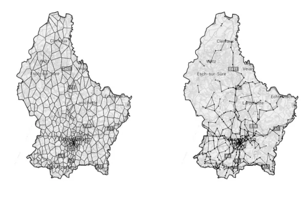
(a) Voronoi Tessellation (b) Convex Hull

Figure 3.3: Coverage area comparison: Voronoi tessellation and simulated locations (rep-resented by their convex hull)

refer to common approximation methods and previous results to confirm the plausibility of the simulation results.

Coverage Area

First, we look at the area covered by each eNodeB in the simulation, i.e. the area within which simulation vehicles were associated with each eNodeB. In Fig. 3.3, we compare the Voronoi tessellation with respect to antenna locations to the convex hulls of each eNodeB’s coverage areas. Each color indicates a different eNodeB, and both plots follow the same color-map. The obvious similarity of both maps confirms that the handover mechanism is working as intended. Inversely, this also shows that the Voronoi tessellation approximates the simulated coverage area, confirming the adequacy of Voronoi tessellation for estimating base station coverage areas. Note that in the simulation, there is overlap between coverage areas, which is likely to increase if additional mechanisms such as power boosting/cell breathing are implemented.

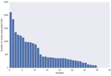
We also looked at the number of unique UEs associated with each eNodeB over the course of a full simulation run. Looking at Fig. 3.4, we can see that there are two eNodeBs that are particulaly frequented. A dozen eNodeBs encounter more than 500 UEs (at 5% LTE equipment rate). The most important eNodeBs are located in the city center and in the south area of the ring, while the remaining two thirds of eNodeBs in the simulation have lower relative importance.

(42)

Figure 3.4: No. of unique associated UEs per simulated eNodeB at 5% equipment rate

Signal Strength - SNR

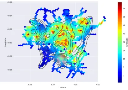
Fig. 3.5 shows color-coded signal strength and the contour of vehicular density levels in a joint representation. The density is evaluated over an entire day, and we can see the highest values on the ring and in the city center, in high coverage areas. In the south-west, we can observe low signal strength and the absence of a nearby eNodeB. However, there are nearby 3G base stations, so this could be due to the progressive equipment upgrade strategy of the mobile network operator.

Fig. 3.6 shows the correlation between the simulated signal-to-noise ratio (SNR) and real, measured RSRP as provided by the free OpenSignal.com Web-API4. We split the scenario territory into squares of 0.25 km2, over which we averaged SNR and queried RSRP from the API, yielding around 100 measurement squares with available data from the required mobile network operator. As discussed by Afroz et al. in [81], SNR is proportional to RSRP in low network load situations, so this comparison is sensible for evaluating the signal strength generated in the scenario. The Pearson coefficientρamounts to 0.317, indicating moderate correlation between both metrics. The differences stem from the very low network load in our evaluation (unlike real data), along with the fact that the emission power of all eNodeBs in the simulation is identical, while it varies in practice (between eNodeBs, but also through cell breathing).

4

(43)

Figure 3.5: SNR vs. vehicular density kernel density estimation

Figure 3.6: Simulated SNR vs. corresponding real RSRP

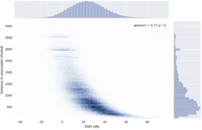
We also evaluated the signal propagation characteristics. Fig. 3.7 shows the joint dis-tribution of SNR and the linear distance to the associated eNodeB. In the central joint distribution plot, we can observe the density following the propagation model’s charac-teristic exponential curve. It shows how closer distance to the eNodeB results in higher SNR values. The variance is due to line of sight and non-line of sight situations due to buildings.

(44)

Figure 3.7: Simulated SNR vs. distance to associated eNodeB

Note that the marginal distribution of SNR (in the histogram at the top) appears to be following a normal distribution, with a mean at around 23dB. As this is close to the commonly used threshold for an excellent signal quality at 20dB5, we can say that half of the values observed correspond to excellent signal conditions, and half of the datapoints correspond to weak to good connection signals.

6.3% of datapoints are located in the <0dB area, which corresponds to edge-of-cell, low connection quality. The distance to the associated eNodeB follows a heavy-tailed distribution. This matches the intuition that the associated eNodeB is more likely to be nearby, with distances less than 1500km representing the majority (around 80%) of cases. The median value of 768m shows that half of the cases are likely urban, where eNodeBs are more densely distributed and thus more likely to be nearby.

Handovers and Dwell Time

We will now evaluate the simulated signalling data from the simulation run, i.e. han-dovers and cell dwell times. Cell dwell times are defined as the time a UE stays associated with an eNodeB before performing a handover. In the work leading up to this study, using floating-car data and using a Voronoi tessellation of 3G and 4G base stations, we have identified a proportionality between squared dwell times and handover counts. A visual-ization of this relationship between the resulting dwell times and handovers is displayed

5

(45)

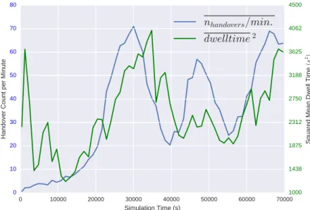
Figure 3.8: Squared mean dwell time vs. Number of handovers per minute

in Fig. 3.8. It shows squared mean dwell time with respect to the time of day (blue line) and the number of handovers per minute (green). Both lines are plotted with 20 minute intervals. Comparing them for the simulated data supports this with a Pearson correlation of ρ = 0.58. This correlation between the number of handovers (∝ flow) and dwell time (∝speed−1_{) indicates that there could be potential for the development of LTE signaling} data-based road traffic estimation system.

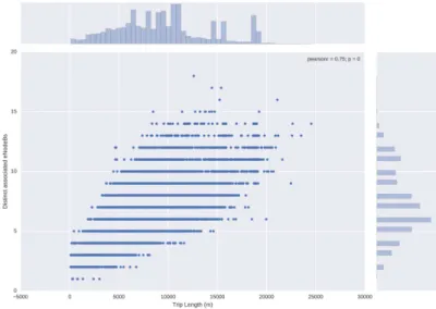
Another interesting signaling metric is that of the number of unique eNodeBs that a vehicle associates with during a trip. In Fig.3.9, we show, for all trips of a day, the distribution of trip lengths and the number of distinct associated eNodeBs that the UE was connected to. The marginal distribution of trip lengths (top histogram) has high variance, showing the large variety in trips in the mobility. The marginal distribution of the number of connected eNodeBs appears to be bi-modal, which could be a characteristic separating trips that are pass by the city center (with high eNodeB density) from suburban and highway trips (with lower eNodeB density).

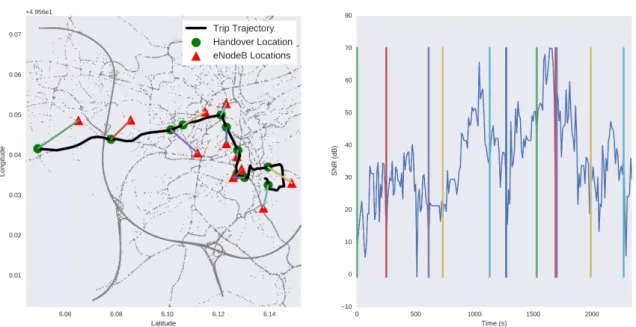
Looking at individual trips allows to further inspect the behavior of handovers in the simulation. Fig. 3.10 consists of two plots that describe a single user trip. The left-hand side plot shows the trajectory of a single vehicle, along with the locations where handovers performed and the associated eNodeBs. Note that the handovers are also visualized using colored lines that match between both plots. The right-side plot shows the SNR evolution