Adaptivity in bayesian inverse finite element problems: learning and simultaneous control of discretisation and sampling errors

materials

Article

Adaptivity in Bayesian Inverse Finite Element

Problems: Learning and Simultaneous Control of

Discretisation and Sampling Errors

Pierre Kerfriden1,2,* , Abhishek Kundu1 and Susanne Claus1,3

1 _{School of Engineering, Cardiff University, The Parade, Cardiff CF243AA, UK;}

[email protected] (A.K.); [email protected] (S.C.)

2 _{MINES ParisTech, PSL University, Centre des Matériaux, BP87 91003 Evry, France}

3 _{Department of Computer Science, University of Copenhagen, Universitetsparken 1,}

2100 Copenhagen, Denmark

* Correspondence: [email protected] or [email protected]

Received: 23 December 2018; Accepted: 5 February 2019; Published: 20 February 2019

Abstract: The local size of computational grids used in partial differential equation (PDE)-based

probabilistic inverse problems can have a tremendous impact on the numerical results. As a consequence, numerical model identification procedures used in structural or material engineering may yield erroneous, mesh-dependent result. In this work, we attempt to connect the field of adaptive methods for deterministic and forward probabilistic finite-element (FE) simulations and the field of FE-based Bayesian inference. In particular, our target setting is that of exact inference, whereby complex posterior distributions are to be sampled using advanced Markov Chain Monte Carlo (MCMC) algorithms. Our proposal is for the mesh refinement to be performed in a goal-oriented manner. We assume that we are interested in a finite subset of quantities of interest (QoI) such as a combination of latent uncertain parameters and/or quantities to be drawn from the posterior predictive distribution. Next, we evaluate the quality of an approximate inversion with respect to these quantities. This is done by running two chains in parallel: (i) the approximate chain and (ii) an enhanced chain whereby the approximate likelihood function is corrected using an efficient deterministic error estimate of the error introduced by the spatial discretisation of the PDE of interest. One particularly interesting feature of the proposed approach is that no user-defined tolerance is required for the quality of the QoIs, as opposed to the deterministic error estimation setting. This is because our trust in the model, and therefore a good measure for our requirement in terms of accuracy, is fully encoded in the prior. We merely need to ensure that the finite element approximation does not impact the posterior distributions of QoIs by a prohibitively large amount. We will also propose a technique to control the error introduced by the MCMC sampler, and demonstrate the validity of the combined mesh and algorithmic quality control strategy.

Keywords: finite element inverse problems; Bayesian statistics; Data-driven modelling; error

estimation; MCMC; machine learning

1. Introduction

The Bayesian statistical framework has been used extensively in the problem of system identification [1] or model updating based on experimental test data [2,3]. The objective of using inverse problems to learn or calibrate model or latent parameters, including model error terms, lies in the fact that underlying parametrised computational models are uncertain, or erroneous [4]. The experimental data when assimilated into the model, using the Bayesian inference framework, is expected to provide joint estimates of the model parameters conditional on the data and compensate for uncertainty/bias

Materials2019,12, 642 2 of 24

in the model predictions. However, operating only in the field of model parameters is problematic for a number of reasons. Firstly, the underlying computational models for any practical application is expensive. As a result working with a very high resolution numerical model at every stage is prohibitively expensive. Secondly, when using surrogate models in the parameter space in conjunction with a simulator, adaptive enrichment of the response surface does not take adaptive mesh refinement within its purview. This is not optimal since ensuring that the model error in the energy norm is bounded in the parameter space requires a uniformly high resolution and increases the associated computational overhead. Lastly the advanced adaptive mesh refinement techniques are rarely used in conjunction with parametric learning using Bayesian inference. There is significant room for improvement in this regard since a simultaneous control of both statistical and discretisation error would lead to substantially improved predictive numerical models both in terms of accuracy and computational efficiency.

At the root or our methodology is the estimation of errors due to the finite element approximation of the partial differential equation (PDE) of interest. Classically, spatial resolution of finite element

models can be adaptively refined (also known as localh-refinement) based on a posteriori error

estimation techniques [5–7], combined with re-meshing strategies. Within this, methods focussing on errors estimated in terms of specific quantities of interest (QoI), rather than the classical energy norm, constitute the goal-oriented adaptivity scheme [8–12], which is of particular interest in the present study. Numerical studies have shown that these give better convergence in the local features of the solution compared to traditional approaches.

Integrating model reduction techniques with finite element model updating techniques has received some attention in recent years [13], where the motivation is to use Bayesian model updating framework with an adaptive scheme of enriching the surrogate response surface. Multistage Bayesian inverse problems are quite important in this respect [14,15] and have important applications for system identification of vibrating systems. The prediction error is an important parameter to be calibrated in such cases, as the authors point out. But the improvement in model predictions, if solely focussed on obtaining the posterior probabilistic parameter estimates or for adaptive enrichment of the response surface in the parameter space, without considering simultaneous enhancement of the resolution of the numerical simulator would be unsatisfactory both from the standpoints of computational accuracy and efficiency.

The forward problem of uncertainty propagation has been investigated extensively for the solution of stochastically parametrised partial differential equations. These range from efficient stochastic Galerkin methods using polynomial chaos basis functions [16–19], stochastic collocation techniques [20,21], Monte-Carlo sampling based methods (and its various improvements) [22–24] and other deterministic sampling methods [25–27]. The main challenge is to obtain a good approximation of the lower order statistical moments of the state vector or specific quantities of interest. On the other hand, advances in the resolution of stochastic inverse problems has become a very active topic in engineering and mathematical research (see e.g., [28]). Scalable Bayesian inversion algorithms for large-scale problems have been investigated [29] and as well as Bayesian inversion to probabilistic robust optimization under uncertainty [30]. The use of adaptive sparse-grid surrogates unified with Bayesian inversion for posterior density estimates of the model or design has also been studied parameters [3,31,32]. This research focuses mostly on the definition of surrogates of the numerical model and having adaptive methods to control the statistical sampling error in the definition of the response surface. Lately there has been some research [33] that defines adaptivity as the local enrichment of the surrogate model and uses error estimation to bound this error, with no mention of spatial discretisation. However, coupling engineering uncertainty quantification (UQ) with an adaptive scheme for goal-oriented finite element model refinement remains a sparsely studied domain and presents significant challenges. It is so both from the problem formulation perspective, owing to the choice of appropriate candidate estimates based on which adaptive model enrichment can be performed, as well as incorporating it into the general formulation of Bayesian inversion.

The main focus of the paper is to develop a robust methodology for the simultaneous control of errors from multiple sources—the goal-oriented finite element error and the uncertainty-driven statistical error—in a Bayesian identification framework for identification system parameters conditional on data (experimental or otherwise). The novel algorithmic approach proposed in this paper consists in running two Markov Chain Monte Carlo algorithms simultaneously to sample the posterior densities of the quantities of interest (component-wise MCMC). The first chain utilises the current finite element model, whilst the second chain runs with a corrected likelihood function that takes into account the discretisation error. The latter quantity may be constructed by making use of a posteriori finite element error estimates available in the literature. At any time during the sampling process, two empirical densities are available and may be compared to evaluate the effect of the discretisation error onto posterior densities. The second building block of our algorithmic methodology allows us to determine whether enough samples have been drawn by the component-wise MCMC. Using multiple parallel chains combined with bootstrap-based estimates of sampling errors, we automatically stop the MCMC algorithms when either (i) the required level of accuracy is achieved or (ii) we have generated enough statistical confidence in the fact that the discretisation error is too large for our purpose, and therefore that mesh refinement is necessary. While any available error estimate of the discretisation error may be used within the general strategy outlined above (a goal-oriented residual or recovery-based error estimate, for instance [8,9,11,34]), we choose instead to construct this estimate via a dedicated machine learning approach. This interesting feature, inspired by previous work in data-driven error modelling [35–38], will be briefly outlined in the paper.

The paper is organised as follows. Section2introduces the Bayesian inverse problem based on a

finite element model of a parametrised vibrating structure. This section also includes discussions on

discretisation error. Some numerical examples are presented in Section3, which aims to demonstrate

the convergence of the joint posterior distributions on the model parameters through successive stages

of mesh refinement. Section4discusses the total error as a combination of statistical and discretisation

error that results from the MCMC algorithm used for sampling from posterior distributions. Section5

gives the methodology for robust, simultaneous control of all error sources within the adaptive inverse problem solver using a component-wise MCMC algorithm in conjunction with bootstrap-aggregated

regression model for model parameters. Numerical examples are presented and discussed in Section6

to demonstrate the capabilities of the proposed methodology. 2. Finite Element Bayesian Inverse Problems

Although the methodology proposed in this paper is general, we will apply it to the verification of popular inverse finite element procedures used to monitor the integrity of structures during service. We will assume that the structure can be modelled as an elastic body, and that potential structural damage can be modelled by the evolution of a field of elastic constants characterised by a finite number of uncertain parameters. Assuming that the resonance frequencies of the structure have been measured physically, we attempt to identify this set of mathematical parameters, through the solution of an inverse problem. Significant deviations from the parameter values corresponding to an undamaged structural state may reveal structural failure. This is a typical condition monitoring method used for non-destructive structural testing.

In order to clarify the proposed study, we will assume that we have measured thendfirst dynamic

eigenfrequenciesd=ln(ω1) ... ln(ωnd)

T

of the structure represented in Figure1. The purpose

of the model inversion is to identify the values ofnµparametersµ=

µ1 ... µnµ

T

of the structural

dynamics model, here the log of the elastic modulii of the subdomains represented in Figure1.

We will also aim to predict the remainingnp−ndfrequencies p =

ln(ωn_d+1) ... ln(ωnd+np)

T .

Materials2019,12, 642 4 of 24

implicitly through the evaluation of a standard finite element model of the steady-state, undamped structural vibrations.

Applied & Computational Mechanics Group E=eµ1 E=eµ2

E

=

e

µ4

E

=

e

µ5 E=eµ6 E= 1 E=eµ3 -2.5 -2 -1.5 -1 -0.5 0 0.5 1 1.5 2 2.5 -2.5 -2 -1.5 -1 -0.5 0 0.5 1 1.5 2 2.5 -1.5 -1 -0.5 0 0.5 0 0.02 0.04 0.06 0.08 0.1 0.12 0.14 0.16 0.18 0.2

!1

!2

Prior µ1 µ3 Forward UP

!3

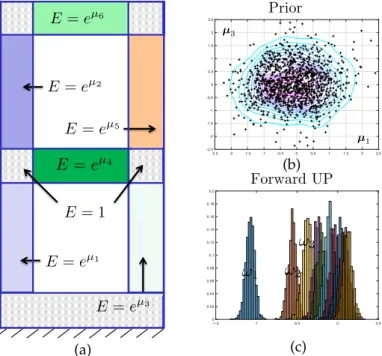
(a) (b) (c)

Figure 1.(a) Structure undergoing structural vibrations. The grey area have a known, deterministic

Young modulus. This property is piecewise constant in the coloured areas, and Gaussian distributed. (b) The corresponding marginal probability density function for two of the 6 parameters is represented in the top-left corner. (c) Standard Monte-Carlo finite element process is employed to compute the distribution of the 10 first free vibration frequencies and represent the marginal distribution of each of these quantities.

2.1. Bayesian Inverse Problem

We assume that the quantities d that are measured experimentally are described by the

mathematical model, up to an error, which is modelled in a probabilistic manner. Following standard Bayesian procedures, this error is modelled as a white Gaussian noise,

d=dm+e, e∼ N(0,Σ−_n1) (1)

withΣ0a positive definite covariance matrix.Ad:µ→dm:=Ad(µ)is the mathematical prediction

that corresponds to the experimental observation. ModelAdis a deterministic function ofnµuncertain

model parameters that we organise in anµ-dimensional vectorµ. Bayesian inversion requires to

associate a prior probability density with the model parametersµ. This prior probability density,

denoted byπµ(µ)in the following, encodes the knowledge that we possess aboutµbefore making

any physical observations.

Seen from a different point of view, the probabilistic inversion setting amounts to the definition of

a joint probability distribution forµandd:

πµ,d(µ,d) =π_d|µ(µ,d)πµ(µ) (2)

The formal expression of likelihood functionL(µ;d) := π_d|µ(µ,d)is a direct consequence of

assumption (1), namely L(µ;d) = q 1 (2π)nd|Σn| e− 1 2 (d−Ad(µ))TΣn−1(d−Ad(µ)) (3)

It is now possible to formally proceed to the inversion itself by conditioning the joint distribution to actually observed quantities. Applying Bayes’ formula, the posterior probability density of the model parameters is

π_µ|d(µ;d) = L(

µ;d)πµ(µ)

πd(d)

(4)

whereπd(d)is a normalising constant, whose computation requires a usually intractable integration.

Bayes formula provides us with an updated knowledge about the uncertain part of our mathematical model. It is now possible to predict unobserved quantities i.e.,

p=Ap(µ), µ∼πµ|d(µ;d) (5)

by formally propagating the posterior uncertainty through modelAp:µ→p_m:=Ap(µ). The posterior

predictive probability density ofpwill be denoted by symbolπ_p|d(µ;d).

2.2. Finite Element Modelling of Inverse Structural Vibration Problems

2.2.1. Direct Finite element Procedure for Frequency-Domain Vibrations The numerical model

µ→A(µ):= Ad(µ) Ap(µ) !

(6)

is implicitly defined through the solution of a continuum mechanics problem. The components ofdm

andpare the logarithm of the eigenvalues corresponding to the following parametrised eigenvalue

problem:Find u∈ H1_{(Ω)andω∈}

R+such that∀v∈ H1(Ω) Z

Ω ∇su:D(x;µ):∇sv dΩ−ω

2Z

Ωρu·v dΩ=0 (7)

In the previous variational statement,Ω is the domain occupied by the structure of interest,

H1_{(Ω)is the space of functions defined overΩ, with values in}

R2, that are zero on part∂uΩof the

boundary of the domain, and whose derivatives up to order one are square integrable.∇sdenotes the

symmetric part of the gradient operator.Dis the fourth order Hooke tensor andρis the mass density

of the solid material. The problem possesses an infinite number of solutions(ω,u)called free vibration

modes. We order the free vibration frequencies in increasing orderω1<ω2< ... <ωnd+np. The free

vibration modes are functions of uncertain material parametersµthrough the definition of the Hooke

tensor. Specifically,

D(x;µ):∇s. =λ(x;µ)Tr(∇s.)I+2G(x;µ)(∇s.) (8)

with the parametrised Lamé constants

λ(x;µ) = 0.3×E(x;µ)

2(1+0.3)(1−2×0.3) and G(x;µ) =

E(x;µ)

2(1+0.3) (9)

Solving the continuum mechanics model is equivalent to evaluating the mapping

µ→ Ad(µ) Ap(µ) ! =    ln ω1(µ) ... ωn_d(µ) T lnωnd+1(µ) ... ωnd+np(µ) T   . (10)

There is, in general, no analytical solution to the continuous vibration problem, and a standard way

to obtain approximate solutions is to substitute a finite element spaceUh_{(Ω)for infinite dimensional}

Materials2019,12, 642 6 of 24

predictive results, while too fine a mesh will lead to numerically intractable results, or, in any case, to a waste of computing resources.

2.2.2. Finite Element Approximation of the Bayesian Inverse Problem

Whilst using the continuum mechanics model exactly would deliver the posterior density

π_µ|d(µ;d)as solution of the Bayesian inverse problem, we now have an approximate posterior density

¯ πµ|d(µ;d) = ¯ L(µ;d)πµ(µ) ¯ π(d) (11)

where the finite element likelihood ¯Lis obtained by substituting finite element mapping ¯Ad for

Ad in Equation (3). Similarly, the approximate posterior density ofp is denoted by ¯π_p|d(µ;d)and

obtained by evaluating finite element mapping ¯Apinstead ofAp when propagating the posterior

uncertainties forward. 2.2.3. Discretisation Error

The finite element error is the mismatch between ¯π_µ|d(µ;d)andπ_µ|d(µ;d)on the one hand, and

¯

π_p|d(µ;d)andπ_p|d(µ;d)on the other hand. Various measures can be used to quantify this mismatch,

amongst which the Hellinger distance, defined by

Dh(π_µ|d(µ), ¯π_µ|d(µ)) = qπ_µ|d(µ)− q ¯ π_µ|d(µ) ₂ (12)

the Kullback-Leibler divergence, the total variation distance and the Kolmogorov-Smirnov (KS) distance, defined by Dks(π_µ|d(µ), ¯π_µ|d(µ)) =sup µ (Π_µ|d(µ)−Π¯µ|d(µ)) (13)

where the capital symbolsΠ.denotes the cumulative probability density corresponding toπ., and ¯Π.

is the finite element approximation ofΠ.. This contribution will make use of the latter measure, in a

one-dimensional setting (i.e., it will be applied to control the accuracy of the posterior density of one of

the elements ofµor one of the elements ofp). The attractiveness of the Kolmogorov–Smirnov distance

is its straightforward application in the context of Monte-Carlo procedures, where only empirical densities are available, and its closeness to confidence intervals (CIs), which makes its values relatively

easy to interpret within the context of a posteriori error estimation. Notice that theDks is lower

bounded by 0 (identical density functions) and upper bounded by 1 (non-overlapping support for the probability density functions).

3. Numerical Examples—Part I: Effect of Discretisation Errors Onto Posterior Densities

This section introduces the numerical examples that will be investigated in this paper, and aims to provide a first qualitative understanding of the effect of mesh refinement onto the quality of posterior probability densities.

3.1. Forward Stochastic Model

The stochastic field of Young’s modulus that will be used to exemplify the error control approach

proposed in this paper is defined via a decomposition of domainΩintonµ+1=7 non-overlapping

subdomains{Ωi}_J1nµ+1K such that

[

i_∈J1nµ+1K

Ωi = Ω and Ωi∩Ωj = { } for i 6= j. The domain

decomposition is represented in Figure1. Then, the proposed model is such that

Hence, the scalar parameters contained in vectorµ ∈ Rnµ are the logarithms of the Young’s

modulii corresponding to each of the subdomains.

The prior density is a multivariate Gaussian, and is given by equation

πµ(µ) = 1 q (2π)nµ|Σ0| e− 1 2 (µ−µ0)TΣ0−1(µ−µ0) (15)

The prior meanµ0is the null vector, and the prior varianceΣ0=σ₀2Id, whereId∈Rnµ×Rnµis

the identity matrix, is diagonal and isotropic. The prior density is represented in dimensions(µ1,µ3)

in Figure1.

Finally, we model the erroreas a zero-mean multivariate Gaussian (consistently with what was

described in previous section), with independent components and isotropic variance, i.e.,Σn=σn2Id.

3.2. Computational Meshes

The evaluation of the likelihood function appearing in solution (11) of the Bayesian inverse problem requires solving the continuum mechanics problem using the finite element method. In this

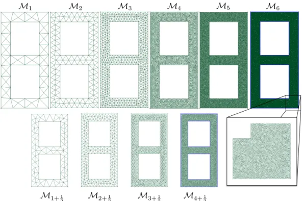
example, we use a sequence of meshes{Mi}i_∈JnmKassociated with a monotonically increasing number

of degrees of freedom. These meshes are represented in Figure2. Although the sequence of meshes is

not strictly hierarchical, we see that the typically uniform element size is divided by≈2 when moving

from meshMito meshMi+1. The intermediate meshes{M_i+1

2}i∈J1 ˜nmKrepresented in Figure2will

be used later on.

Applied & Computational Mechanics Group

Figure 2.Hierarchy of computational meshes used in the study. We aim at selecting the coarsest mesh

that delivers the targeted distributions up to a user-defined numerical accuracy. The second line of meshes is only used for error estimation purposes.

3.3. Inverse Problems and First Results

Two tests will now be investigated:

• Test 1(weakly informative data): only the first eigenvalue is measured, i.e.,dis scalar. This can be

Materials2019,12, 642 8 of 24

• Test 2 (strongly informative data): the first three eigenvalues of the structure are measured.

This can be interpreted as an inverse problem, where rich information is used to identify all the unknown of the model, and the probabilistic setting acts as a regulariser.

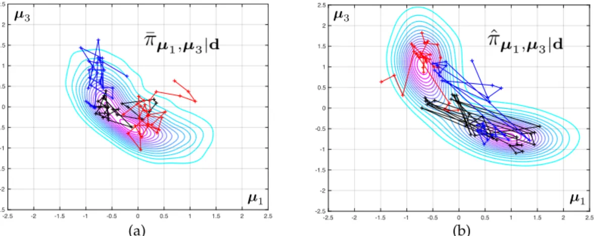
The two corresponding marginal posterior density ˆπ_µ1,µ3|dobtained when using meshM3are

represented in Figure3. Samples from this density are obtained by a Monte-Carlo sampler, as presented

in next section. A Kernel Density Estimate (KDE) is used as a smoother for illustration purposes only. Notice that for the predictive posterior densities, the histograms correspond to the marginal densities of each individual eigenvalue, which explains their overlap.

Applied & Computational Mechanics Group -1.5 -1 -0.5 0 0.5 0 0.05 0.1 0.15 0.2 0.25 0.3 -2.5 -2 -1.5 -1 -0.5 0 0.5 1 1.5 2 2.5 -2.5 -2 -1.5 -1 -0.5 0 0.5 1 1.5 2 2.5

µ

1

µ

3

!

1

!

2

!

3

Data

Posterior

-2.5 -2 -1.5 -1 -0.5 0 0.5 1 1.5 2 2.5 -2.5 -2 -1.5 -1 -0.5 0 0.5 1 1.5 2 2.5 -1.5 -1 -0.5 0 0.5 0 0.02 0.04 0.06 0.08 0.1 0.12 0.14 0.16 0.18 0.2

Data

Posterior

µ

₁

µ

₃

!

1

!

2

!

3

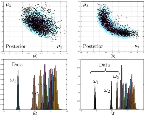
(a) (b) (c) (d)

Figure 3. (a) Joint posterior probability distribution for two of the 6 unknown elastic modulii and

(c) marginal posterior predictive distributions of the first 10 free vibration frequencies. The data set consists of a noisy measurement of the first frequency only, resulting in fat posterior densities. (b) Posterior distribution of the two unknown elastic modulii when the first 3 vibration frequencies are used as dataset, which results as in much thinner posterior densities. (d) Corresponding posterior predictive densities.

It is interesting to notice that the posterior densities observed in Test 2 are much sharper than that of Test 1, owing to the quality of the data. The symmetry in the results are a consequence of structural

and probabilistic symmetries (see Figure1and the definition of the prior probability density).

Synthetic data for this problem is generated by computing the average of the spectra delivered by

meshesM2andM₂₊1

2, for a reference parameter vectorµd6=µ0but situated in the vicinity of the

prior mode. The model averaging, together with selecting relatively coarse finite element meshes in

sequence{Mi}i∈J nmK, is meant to circumvent the “inverse crime" problem.

3.4. Convergence with Mesh Refinement

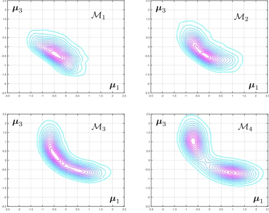
The posterior densities corresponding to Test 2 and to various level of mesh refinement are

displayed in Figure4. The difference between the modes of the predicted eigenvalues that are obtained

number is to be expected as the spatial wave length of the deformations in the continuum can be shown to increase linearly with the eigenfrequency. As a consequence, a good mesh for the first range of frequencies might be unable to capture the faster spatial variations associated with higher vibration mode.

Applied & Computational Mechanics Group -2.5 -2 -1.5 -1 -0.5 0 0.5 1 1.5 2 2.5 -2.5 -2 -1.5 -1 -0.5 0 0.5 1 1.5 2 2.5

µ

₁

µ

₃ -2.5 -2 -1.5 -1 -0.5 0 0.5 1 1.5 2 2.5 -2.5 -2 -1.5 -1 -0.5 0 0.5 1 1.5 2 2.5

µ

₁

µ

₃ -2.5 -2 -1.5 -1 -0.5 0 0.5 1 1.5 2 2.5 -2.5 -2 -1.5 -1 -0.5 0 0.5 1 1.5 2 2.5

µ

₁

µ

₃ -2.5 -2 -1.5 -1 -0.5 0 0.5 1 1.5 2 2.5 -2.5 -2 -1.5 -1 -0.5 0 0.5 1 1.5 2 2.5

µ

₁

µ

₃

Figure 4.Evolution of the joint posterior density of two of the unknown elasticity parameters as the

computational mesh is progressively refined fromM1toM4.

The difference between the posteriori densities corresponding to meshes M3 and M4 is

qualitatively small. The solution of the Bayesian inverse problem converges with mesh refinement. Notice that the posterior distribution for the model parameters goes from mono-modal to multi-modal, which may prove a stumbling block when selecting an appropriate Monte-Carlo sampler.

4. Monte-Carlo Sampler and Combined Effect of Statistical and Discretisation Errors

4.1. Tempered Metropolis-Hastings Markov Chain Monte Carlo Algorithm

The approximate posterior density described by Equation (11) is an arbitrarily complex function

ofµ, as it depends on thenonlinearcomputational model(Ad(µ)TAp(µ)T)T. In particular, standard

random number generators cannot be used to draw samples from this distribution. Importance Monte-Carlo procedures whereby the prior distribution is used as proposal density, will also fail. This is because the posterior density may be arbitrarily different from the prior density, resulting in unacceptably large variances of importance sampling estimates. Designing better proposal densities a priori is impossible and a successful importance sampling approach would require generating the proposal density using advanced methods such as sequential Monte-Carlo samplers.

One of the simplest and generic generator of samples from posterior densities is the

Materials2019,12, 642 10 of 24

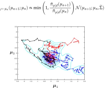
The algorithm works as follows. Starting from sample µn, the next sample µn+1 is drawn from

transitional distribution Tµn+1←µn(µn+1;µn)∝min 1, ¯ π_µ|d(µn+1) ¯ π_µ|d(µn) ! N(µn+1;µn,Σe) (16)

Applied & Computational Mechanics Group -2.5 -2 -1.5 -1 -0.5 0 0.5 1 1.5 2 2.5 -2.5 -2 -1.5 -1 -0.5 0 0.5 1 1.5 2 2.5

µ

₁ µ3

Figure 5.Three independent MCMC chains sampling a multivariate Gaussian distribution.

This is done by first drawing a random move from µk using the multivariate Gaussian

(any proposal can be used, but the expressions exposed in this section are only valid for symmetric proposals), and then accepting or rejecting the move in order to account for the first term of the transition. Typically, a move ending up in a state of higher posterior density is always accepted, whilst a move ending up in a state of lower density may be accepted or not, depending on the result of a die and the ratio of posterior densities between current and proposed states.

This particular transition is designed such that the following ergodic property holds:

Z

µn+1

Tµn+1←µn(µn+1;µn)dµn=π¯µ|d(µn+1) (17)

As a result, under some assumptions, the Markov chain is guaranteed to have ¯π_µ|das its stationary

distribution, which means thatµn ∼π¯_µ|dasn→∞. Each sample, taken individually, is distributed

according to the posterior density, if the chain is run long enough. Due to the Markov process, the samples are not independent, which makes frequentist error estimation and convergence diagnosis more difficult than in the context of traditional Monte-Carlo algorithm, where tools such as standard error and bootstrap apply without particular difficulty. Practically, a burn-in phase is first observed,

whereby the chain “seeks” the regions of high probability densities (see Figure5). Once found, samples

become progressively distributed according to the target posterior density.

Notice thatΣe is difficult to choose a priori. Adaptive proposal MCMC have been proposed

in [40,41]. Alternative solutions to choose good proposal are methods based on particle mechanics (e.g., Langevin diffusion, Hamiltonian dynamics) (see e.g., [42]). In this particular contribution, the proposal densities have been calibrated “by hand”. We use a tempered version of the MCMC algorithm, whereby we simultaneously sample multiple tempered replicates of the posterior density, with proposed state exchange between replicates that are subsequently Metropolis corrected [43,44] (see also [45] for an interesting application in the context of structural damage assessment). This relatively classical MCMC algorithm allows us to sample from; densities that are multi-modal or become multi-modal with mesh refinement (at least in the low-dimensional parametric settings that is investigated in this paper, as multi-modality in high-dimensions remains an open problem).

The call to the finite element solver is hidden in the acceptance/rejection test, which requires the evaluation of the finite element likelihood at the proposed state. Therefore, as for a standard MC algorithm, one iteration means one evaluation of the computational model.

4.2. Empirical Posterior Densities

Once n samples M˜ = {µ1,µ2, ... ,µn} have been computed (n larger than 10) by the MH

algorithm, we discard the first 25% (burn-in) of these samples, resulting in ˜nsamples that we hope are

located in the ergodic part of the Markov chain. The resulting empirical probability density is given by ¯ π_µ|d(µ)≈π¯(n) µ|d(µ):= 1 ˜ n n

∑

k=n−n+1˜ δ(µ−µk) (18)

whereδis the Dirac delta function. Accordingly, the empirical predictive posterior density is

¯ π_p|d(p)≈π¯_p(n)_|d(p):= 1 ˜ n n

∑

k=n−n+1˜ δ(p−Ap(µk)) (19)

The cumulative empirical predictive posterior density may be expressed as ¯ Πµ|d=d(µ):= 1 ˜ n n

∑

k=n−n+1˜ I(µ;µk≤µ) (20)

whereIis the indicator function, and the inequality is to be understood in a component-by-component

manner. A similar definition holds for the cumulative posterior density ofp.

4.3. Total Error Measure

It is now clear that both the finite element discretisation and the Monte-Carlo approximate sampling affect the quality of the resulting posterior densities. The total error, for the marginal

distribution of a single elementµiofµ, reads as

Dks(π_µi|d(µi), ¯π(n) µi|d(µi)) =sup µi _(Π µi|d(µi)−Π¯ (n) µi|d(µi)) (21)

which can be formally decomposed as follows

Dks(π_µi|d(µi), ¯π(n) µi|d(µi)) = sup µi (Π_µi|d(µi)−Π¯µi|d(µi)) +Π¯µi|d(µi)−Π¯ (n) µi|d(µi)) ≤ Dks(π_µi|d(µi), ¯π_µi|d(µi)) +Dks(π¯_µi|d(µi), ¯πmc_µi|d(µi)) (22)

In the last expression, the first term is the pure finite element error, which would occur if we could run the Markov process for an infinite number of iterations, while the second term is a pure statistical error.

We also define the error of an elementpiofpas follows:

Dks(π_pi|d(pi), ¯π(n)_p i|d(µi)) =sup pi (Πpi|d(pi)−Π¯(n)_pi|d(pi)) (23)

5. Robust, Automatised and Comprehensive Error Control

5.1. Simulation of the Discretisation Error

The finite element method introduces an error in computational mapping A(µ) =

Ad(µ)T Ap(µ)T T

. MappingAcontains all the scalar quantities that need to be evaluated through

calls to the finite element solver, namely the numerical predictions of the physical measurementsd,

and the posterior predictionsp. We define the error in the simulated data as

Materials2019,12, 642 12 of 24

and the error in the posteriori predictions as

∆Ap(µ) =Ap(µ)−A¯p(µ) (25)

For now, we assume that both these quantities can be estimated, at affordable numerical cost and

in a reliable manner. Therefore, for any value of parameterµ, a corrected computational model is

available, which reads as

Ad(µ) Ap(µ) ! ≈ very close to ˆ Ad(µ) ˆ Ap(µ) ! := A¯_¯d(µ) Ap(µ) ! + ∆Acd(µ) c ∆Ap(µ) ! (26)

where symbolb. denotes computable estimates.

5.2. Component-Wise MCMC

It is now posible to sample the corrected posterior distribution ˆ π_µ|d(µ;d) = ˆ L(µ;d)πµ(µ) ˆ π(d) (27)

using MCMC. It should be clear that the corrected posterior distribution is simply obtained by replacing the corrected computational model (26) into the expression of the likelihood function, Equation (3). Notice that the normalising constant is affected by modifications of the computational model. This is of no practical consequence as MCMC samplers work with unnormalised densities, and the KS distance uses empirical cumulative distributions directly, without the need for smoothing or marginalisation. We formally define a component-wise MCMC were the uncorrected and corrected computational models are sampled at the same time. This will yield an estimate of the effect of the discretisation error on posteriori densities at any stage of the Markov process, which, in turn, will allow us to develop an early-stopping methodology. The Component-wise MCMC iteration proceeds as follows, given a

current sample(µ¯n, ˆµn)of the uncorrected/corrected finite element posteriori densities,

• Draw(µ¯n+1, ˆµn+1)such that

¯

µn+1∼ N(. ; ¯µn,Σe) and µˆn+1∼ N(. ; ˆµn,Σe) (28)

• draw(u,v)such that

u∼ U([0 1]) and v∼ U([0 1]) (29)

• Accept ¯µn+1if and only if

u≤min 1,L¯(µ_¯¯n+1;d)πµ(µ¯n+1)

L(µ¯n;d)πµ(µ¯n)

!

(30)

set ¯µn+1=µ¯kotherwise.

• Accept ˆµn+1if and only if

v≤min 1,Lb(µˆn+1;d)πµ(µˆn+1) b L(µˆn;d)πµ(µˆn) ! (31) set ˆµn+1=µˆkotherwise.

The MCMC algorithm is initialised by state(µ¯0, ˆµ0), where both(µ¯0and ˆµ0)are drawn from

distributionπ0.

In the field of a posteriori finite element error estimation, the error estimate is usually

non-Markovian Monte-Carlo samplers, by post-processing each of the independent samples. Here, unfortunately, the finite element model has to be called twice at every iteration of the Markov process. Whether this can be avoided or not, for instance by making use of elements of sequential Monte-Carlo samplers, is unclear to us at this stage.

5.3. Machine Learning-Based Simulation of the Discretisation Error

At this stage, any numerical error estimator can be used, provided that it is goal-oriented. A method of choice could be a residual-based [5,6] or smoothing-based a posteriori error estimator [12,46] in conjunction with the adjoint methodology [8,9,11]. In addition, nothing prevents us from using a meta-modelling approach, such as projection-based reduced order modelling [47–52] or polynomial chaos expansions [16,17] to approximate the variations of the computed quantities of interest with parameter variation. Error estimates also exist for such two-level approximations.

In this contribution, we develop and use a feature-based method, that finds its roots in data-science methodologies and is much more “black-box” than the previously mentioned strategies. The proposed technique is inspired by the work of [35–37].

The exact continuum mechanics model is well approximated by a very refined numerical strategy (e.g., no meta-modelling and a very fine mesh). However, this very refined numerical model cannot be used at every iteration of MCMC as its evaluation is very costly. We propose to train a model that will

map parameterµto the output of the generally intractable very fine model through the combination of

(i) a dedicated feature extractor and (ii) a weakly parametric regression model. This combination is defined as A?_d(µ) A?p(µ) ! − A¯_¯d(µ) Ap(µ) ! = wished c ∆Ad(µ) c ∆Ap(µ) ! = constructedR(F(µ);θ) (32)

where the .?denote quantities that are delivered by the overkill (but computable) numerical model and

Ris a weakly parametrised regression model, here a neural network regression (a Gaussian process

could be used as well, but a random forest would probably have been the most efficient choice, given the way we bootstrap the regression model to generate estimates of generalisation errors), parametrised

by a set of parametersθ ∈Rnθ (we do not explicitly distinguish parameters and hyper-parameters

in our notations).Fis a mapping from inputµto a feature space. Its careful design is critical to the

success of the machine learning procedure. We choose to construct the following features:

F(µ) =      ˜ Ad(µ)−A¯d(µ) ¯ Ad(µ) ˜ Ap(µ)−A¯p(µ) ¯ Ap(µ)      (33)

where ˜Ad(µ)areslighltycorrected computational models, here generated by refining the mesh by a

moderate factor. In our examples, the typical mesh size is divided by 1.5 (see Figures2and6where

we use meshM_i+1

2 to correct meshMi, whilst the overkill solution is computed usingMi+2). In this

fashion, the generation of features will remain of the order of the computation of the finite element solution itself.

Materials2019,12, 642 Applied & Computational 14 of 24 Mechanics Group O ff lin e: M ac hi ne l ear ni ng Online feature evaluation -0.075 -0.07 -0.065 -0.06 -0.055 -0.05 -0.27 -0.26 -0.25 -0.24 -0.23 -0.22 -0.21 -0.2 -0.19 -2 -4 0 2 4 -2 6 8 4 0 10 2 0 2 -2 4 -4 -0.26 -0.25 -1.8 -0.24 -0.23 -0.22 -0.21 -2 -0.2 -0.19 -2.2 _-0.05 -0.055 -2.4 _-0.065 -0.06 -0.07 -2.6 _-0.075 eT₁ A?_p <latexit sha1_base64="lerOz5cyhkDktY2tS+drNnLevHU=">AAACIHicbVDLTgIxFO3gC/GFunTTSExckRljgkt8LFxqImDCwKRTLtDQeaS9YyST+RQ3/oobFxqjO/0ay8BCxZM0PT3n3vTe48dSaLTtT6uwsLi0vFJcLa2tb2xulbd3mjpKFIcGj2Skbn2mQYoQGihQwm2sgAW+hJY/Op/4rTtQWkThDY5j6ARsEIq+4AyN5JVrrh/JXgqZ53RvaP7Q48BcqXsBElk29U8zz0W4xzTOuq5Gprxyxa7aOeg8cWakQma48sofbi/iSQAhcsm0bjt2jJ2UKRRcQlZyEw0x4yM2gLahIQtAd9J8wYweGKVH+5EyJ0Saqz87UhboydimMmA41H+9ifif106wf9JJRRgnCCGfftRPJMWITtKiPaGAoxwbwrgSZlbKh0wxjibTkgnB+bvyPGkeVR276lwfV+pnsziKZI/sk0PikBqpk0tyRRqEkwfyRF7Iq/VoPVtv1vu0tGDNenbJL1hf31DKpPA=</latexit> <latexit sha1_base64="lerOz5cyhkDktY2tS+drNnLevHU=">AAACIHicbVDLTgIxFO3gC/GFunTTSExckRljgkt8LFxqImDCwKRTLtDQeaS9YyST+RQ3/oobFxqjO/0ay8BCxZM0PT3n3vTe48dSaLTtT6uwsLi0vFJcLa2tb2xulbd3mjpKFIcGj2Skbn2mQYoQGihQwm2sgAW+hJY/Op/4rTtQWkThDY5j6ARsEIq+4AyN5JVrrh/JXgqZ53RvaP7Q48BcqXsBElk29U8zz0W4xzTOuq5Gprxyxa7aOeg8cWakQma48sofbi/iSQAhcsm0bjt2jJ2UKRRcQlZyEw0x4yM2gLahIQtAd9J8wYweGKVH+5EyJ0Saqz87UhboydimMmA41H+9ifif106wf9JJRRgnCCGfftRPJMWITtKiPaGAoxwbwrgSZlbKh0wxjibTkgnB+bvyPGkeVR276lwfV+pnsziKZI/sk0PikBqpk0tyRRqEkwfyRF7Iq/VoPVtv1vu0tGDNenbJL1hf31DKpPA=</latexit> <latexit sha1_base64="lerOz5cyhkDktY2tS+drNnLevHU=">AAACIHicbVDLTgIxFO3gC/GFunTTSExckRljgkt8LFxqImDCwKRTLtDQeaS9YyST+RQ3/oobFxqjO/0ay8BCxZM0PT3n3vTe48dSaLTtT6uwsLi0vFJcLa2tb2xulbd3mjpKFIcGj2Skbn2mQYoQGihQwm2sgAW+hJY/Op/4rTtQWkThDY5j6ARsEIq+4AyN5JVrrh/JXgqZ53RvaP7Q48BcqXsBElk29U8zz0W4xzTOuq5Gprxyxa7aOeg8cWakQma48sofbi/iSQAhcsm0bjt2jJ2UKRRcQlZyEw0x4yM2gLahIQtAd9J8wYweGKVH+5EyJ0Saqz87UhboydimMmA41H+9ifif106wf9JJRRgnCCGfftRPJMWITtKiPaGAoxwbwrgSZlbKh0wxjibTkgnB+bvyPGkeVR276lwfV+pnsziKZI/sk0PikBqpk0tyRRqEkwfyRF7Iq/VoPVtv1vu0tGDNenbJL1hf31DKpPA=</latexit> <latexit sha1_base64="lerOz5cyhkDktY2tS+drNnLevHU=">AAACIHicbVDLTgIxFO3gC/GFunTTSExckRljgkt8LFxqImDCwKRTLtDQeaS9YyST+RQ3/oobFxqjO/0ay8BCxZM0PT3n3vTe48dSaLTtT6uwsLi0vFJcLa2tb2xulbd3mjpKFIcGj2Skbn2mQYoQGihQwm2sgAW+hJY/Op/4rTtQWkThDY5j6ARsEIq+4AyN5JVrrh/JXgqZ53RvaP7Q48BcqXsBElk29U8zz0W4xzTOuq5Gprxyxa7aOeg8cWakQma48sofbi/iSQAhcsm0bjt2jJ2UKRRcQlZyEw0x4yM2gLahIQtAd9J8wYweGKVH+5EyJ0Saqz87UhboydimMmA41H+9ifif106wf9JJRRgnCCGfftRPJMWITtKiPaGAoxwbwrgSZlbKh0wxjibTkgnB+bvyPGkeVR276lwfV+pnsziKZI/sk0PikBqpk0tyRRqEkwfyRF7Iq/VoPVtv1vu0tGDNenbJL1hf31DKpPA=</latexit>

e<latexit sha1_base64="jc3XBQtHX0sOcN/4Cc4xObSGJdc=">AAACJHicbVDLSsNAFJ34tr6qLt0MFsFVSURQcONr4bJCq4Umhsnk1g5OHszcqCXkY9z4K25c+MCFG7/FaZuFWi8MczjnXO69J0il0Gjbn9bE5NT0zOzcfGVhcWl5pbq6dqGTTHFo8UQmqh0wDVLE0EKBEtqpAhYFEi6Dm5OBfnkLSoskbmI/BS9i17HoCs7QUH71wA0SGeZQ+M5Vk7p3IoQew3zI6n5kvtw9BYmsGBmPisJ3Ee4xTwu/WrPr9rDoOHBKUCNlNfzqmxsmPIsgRi6Z1h3HTtHLmULBJRQVN9OQMn7DrqFjYMwi0F4+PLKgW4YJaTdR5sVIh+zPjpxFerCxcUYMe/qvNiD/0zoZdve9XMRphhDz0aBuJikmdJAYDYUCjrJvAONKmF0p7zHFOJpcKyYE5+/J4+Bip+7Yded8t3Z4XMYxRzbIJtkmDtkjh+SMNEiLcPJAnsgLebUerWfr3foYWSessmed/Crr6xvyj6be</latexit><latexit sha1_base64="jc3XBQtHX0sOcN/4Cc4xObSGJdc=">AAACJHicbVDLSsNAFJ34tr6qLt0MFsFVSURQcONr4bJCq4Umhsnk1g5OHszcqCXkY9z4K25c+MCFG7/FaZuFWi8MczjnXO69J0il0Gjbn9bE5NT0zOzcfGVhcWl5pbq6dqGTTHFo8UQmqh0wDVLE0EKBEtqpAhYFEi6Dm5OBfnkLSoskbmI/BS9i17HoCs7QUH71wA0SGeZQ+M5Vk7p3IoQew3zI6n5kvtw9BYmsGBmPisJ3Ee4xTwu/WrPr9rDoOHBKUCNlNfzqmxsmPIsgRi6Z1h3HTtHLmULBJRQVN9OQMn7DrqFjYMwi0F4+PLKgW4YJaTdR5sVIh+zPjpxFerCxcUYMe/qvNiD/0zoZdve9XMRphhDz0aBuJikmdJAYDYUCjrJvAONKmF0p7zHFOJpcKyYE5+/J4+Bip+7Yded8t3Z4XMYxRzbIJtkmDtkjh+SMNEiLcPJAnsgLebUerWfr3foYWSessmed/Crr6xvyj6be</latexit><latexit sha1_base64="jc3XBQtHX0sOcN/4Cc4xObSGJdc=">AAACJHicbVDLSsNAFJ34tr6qLt0MFsFVSURQcONr4bJCq4Umhsnk1g5OHszcqCXkY9z4K25c+MCFG7/FaZuFWi8MczjnXO69J0il0Gjbn9bE5NT0zOzcfGVhcWl5pbq6dqGTTHFo8UQmqh0wDVLE0EKBEtqpAhYFEi6Dm5OBfnkLSoskbmI/BS9i17HoCs7QUH71wA0SGeZQ+M5Vk7p3IoQew3zI6n5kvtw9BYmsGBmPisJ3Ee4xTwu/WrPr9rDoOHBKUCNlNfzqmxsmPIsgRi6Z1h3HTtHLmULBJRQVN9OQMn7DrqFjYMwi0F4+PLKgW4YJaTdR5sVIh+zPjpxFerCxcUYMe/qvNiD/0zoZdve9XMRphhDz0aBuJikmdJAYDYUCjrJvAONKmF0p7zHFOJpcKyYE5+/J4+Bip+7Yded8t3Z4XMYxRzbIJtkmDtkjh+SMNEiLcPJAnsgLebUerWfr3foYWSessmed/Crr6xvyj6be</latexit><latexit sha1_base64="jc3XBQtHX0sOcN/4Cc4xObSGJdc=">AAACJHicbVDLSsNAFJ34tr6qLt0MFsFVSURQcONr4bJCq4Umhsnk1g5OHszcqCXkY9z4K25c+MCFG7/FaZuFWi8MczjnXO69J0il0Gjbn9bE5NT0zOzcfGVhcWl5pbq6dqGTTHFo8UQmqh0wDVLE0EKBEtqpAhYFEi6Dm5OBfnkLSoskbmI/BS9i17HoCs7QUH71wA0SGeZQ+M5Vk7p3IoQew3zI6n5kvtw9BYmsGBmPisJ3Ee4xTwu/WrPr9rDoOHBKUCNlNfzqmxsmPIsgRi6Z1h3HTtHLmULBJRQVN9OQMn7DrqFjYMwi0F4+PLKgW4YJaTdR5sVIh+zPjpxFerCxcUYMe/qvNiD/0zoZdve9XMRphhDz0aBuJikmdJAYDYUCjrJvAONKmF0p7zHFOJpcKyYE5+/J4+Bip+7Yded8t3Z4XMYxRzbIJtkmDtkjh+SMNEiLcPJAnsgLebUerWfr3foYWSessmed/Crr6xvyj6be</latexit> T₁ dAp

eT1 gAp <latexit sha1_base64="srrMnQilGNbkc/yTNFVrcXzEl8s=">AAACJnicbVDLSsNAFJ3UV62vqks3g0VwVRIRdCPUx8JlBatCE8NkcqtDJw9mbtQS8jVu/BU3Lioi7vwUp2kXvi4MczjnXO69J0il0GjbH1Zlanpmdq46X1tYXFpeqa+uXegkUxw6PJGJugqYBili6KBACVepAhYFEi6D/vFIv7wDpUUSn+MgBS9iN7HoCc7QUH79wA0SGeZQ+M71OXXvRQgoZAh5yetBZL7cPQGJrBhbD4vCdxEeME8Lv96wm3ZZ9C9wJqBBJtX260M3THgWQYxcMq27jp2ilzOFgksoam6mIWW8z26ga2DMItBeXp5Z0C3DhLSXKPNipCX7vSNnkR5tbJwRw1v9WxuR/2ndDHv7Xi7iNEOI+XhQL5MUEzrKjIZCAUc5MIBxJcyulN8yxTiaZGsmBOf3yX/BxU7TsZvO2W6jdTSJo0o2yCbZJg7ZIy1yStqkQzh5JM9kSF6tJ+vFerPex9aKNelZJz/K+vwCsKenxw==</latexit> <latexit sha1_base64="srrMnQilGNbkc/yTNFVrcXzEl8s=">AAACJnicbVDLSsNAFJ3UV62vqks3g0VwVRIRdCPUx8JlBatCE8NkcqtDJw9mbtQS8jVu/BU3Lioi7vwUp2kXvi4MczjnXO69J0il0GjbH1Zlanpmdq46X1tYXFpeqa+uXegkUxw6PJGJugqYBili6KBACVepAhYFEi6D/vFIv7wDpUUSn+MgBS9iN7HoCc7QUH79wA0SGeZQ+M71OXXvRQgoZAh5yetBZL7cPQGJrBhbD4vCdxEeME8Lv96wm3ZZ9C9wJqBBJtX260M3THgWQYxcMq27jp2ilzOFgksoam6mIWW8z26ga2DMItBeXp5Z0C3DhLSXKPNipCX7vSNnkR5tbJwRw1v9WxuR/2ndDHv7Xi7iNEOI+XhQL5MUEzrKjIZCAUc5MIBxJcyulN8yxTiaZGsmBOf3yX/BxU7TsZvO2W6jdTSJo0o2yCbZJg7ZIy1yStqkQzh5JM9kSF6tJ+vFerPex9aKNelZJz/K+vwCsKenxw==</latexit> <latexit sha1_base64="srrMnQilGNbkc/yTNFVrcXzEl8s=">AAACJnicbVDLSsNAFJ3UV62vqks3g0VwVRIRdCPUx8JlBatCE8NkcqtDJw9mbtQS8jVu/BU3Lioi7vwUp2kXvi4MczjnXO69J0il0GjbH1Zlanpmdq46X1tYXFpeqa+uXegkUxw6PJGJugqYBili6KBACVepAhYFEi6D/vFIv7wDpUUSn+MgBS9iN7HoCc7QUH79wA0SGeZQ+M71OXXvRQgoZAh5yetBZL7cPQGJrBhbD4vCdxEeME8Lv96wm3ZZ9C9wJqBBJtX260M3THgWQYxcMq27jp2ilzOFgksoam6mIWW8z26ga2DMItBeXp5Z0C3DhLSXKPNipCX7vSNnkR5tbJwRw1v9WxuR/2ndDHv7Xi7iNEOI+XhQL5MUEzrKjIZCAUc5MIBxJcyulN8yxTiaZGsmBOf3yX/BxU7TsZvO2W6jdTSJo0o2yCbZJg7ZIy1yStqkQzh5JM9kSF6tJ+vFerPex9aKNelZJz/K+vwCsKenxw==</latexit> <latexit sha1_base64="srrMnQilGNbkc/yTNFVrcXzEl8s=">AAACJnicbVDLSsNAFJ3UV62vqks3g0VwVRIRdCPUx8JlBatCE8NkcqtDJw9mbtQS8jVu/BU3Lioi7vwUp2kXvi4MczjnXO69J0il0GjbH1Zlanpmdq46X1tYXFpeqa+uXegkUxw6PJGJugqYBili6KBACVepAhYFEi6D/vFIv7wDpUUSn+MgBS9iN7HoCc7QUH79wA0SGeZQ+M71OXXvRQgoZAh5yetBZL7cPQGJrBhbD4vCdxEeME8Lv96wm3ZZ9C9wJqBBJtX260M3THgWQYxcMq27jp2ilzOFgksoam6mIWW8z26ga2DMItBeXp5Z0C3DhLSXKPNipCX7vSNnkR5tbJwRw1v9WxuR/2ndDHv7Xi7iNEOI+XhQL5MUEzrKjIZCAUc5MIBxJcyulN8yxTiaZGsmBOf3yX/BxU7TsZvO2W6jdTSJo0o2yCbZJg7ZIy1yStqkQzh5JM9kSF6tJ+vFerPex9aKNelZJz/K+vwCsKenxw==</latexit> eT₁ gAp <latexit sha1_base64="srrMnQilGNbkc/yTNFVrcXzEl8s=">AAACJnicbVDLSsNAFJ3UV62vqks3g0VwVRIRdCPUx8JlBatCE8NkcqtDJw9mbtQS8jVu/BU3Lioi7vwUp2kXvi4MczjnXO69J0il0GjbH1Zlanpmdq46X1tYXFpeqa+uXegkUxw6PJGJugqYBili6KBACVepAhYFEi6D/vFIv7wDpUUSn+MgBS9iN7HoCc7QUH79wA0SGeZQ+M71OXXvRQgoZAh5yetBZL7cPQGJrBhbD4vCdxEeME8Lv96wm3ZZ9C9wJqBBJtX260M3THgWQYxcMq27jp2ilzOFgksoam6mIWW8z26ga2DMItBeXp5Z0C3DhLSXKPNipCX7vSNnkR5tbJwRw1v9WxuR/2ndDHv7Xi7iNEOI+XhQL5MUEzrKjIZCAUc5MIBxJcyulN8yxTiaZGsmBOf3yX/BxU7TsZvO2W6jdTSJo0o2yCbZJg7ZIy1yStqkQzh5JM9kSF6tJ+vFerPex9aKNelZJz/K+vwCsKenxw==</latexit> <latexit sha1_base64="srrMnQilGNbkc/yTNFVrcXzEl8s=">AAACJnicbVDLSsNAFJ3UV62vqks3g0VwVRIRdCPUx8JlBatCE8NkcqtDJw9mbtQS8jVu/BU3Lioi7vwUp2kXvi4MczjnXO69J0il0GjbH1Zlanpmdq46X1tYXFpeqa+uXegkUxw6PJGJugqYBili6KBACVepAhYFEi6D/vFIv7wDpUUSn+MgBS9iN7HoCc7QUH79wA0SGeZQ+M71OXXvRQgoZAh5yetBZL7cPQGJrBhbD4vCdxEeME8Lv96wm3ZZ9C9wJqBBJtX260M3THgWQYxcMq27jp2ilzOFgksoam6mIWW8z26ga2DMItBeXp5Z0C3DhLSXKPNipCX7vSNnkR5tbJwRw1v9WxuR/2ndDHv7Xi7iNEOI+XhQL5MUEzrKjIZCAUc5MIBxJcyulN8yxTiaZGsmBOf3yX/BxU7TsZvO2W6jdTSJo0o2yCbZJg7ZIy1yStqkQzh5JM9kSF6tJ+vFerPex9aKNelZJz/K+vwCsKenxw==</latexit> <latexit sha1_base64="srrMnQilGNbkc/yTNFVrcXzEl8s=">AAACJnicbVDLSsNAFJ3UV62vqks3g0VwVRIRdCPUx8JlBatCE8NkcqtDJw9mbtQS8jVu/BU3Lioi7vwUp2kXvi4MczjnXO69J0il0GjbH1Zlanpmdq46X1tYXFpeqa+uXegkUxw6PJGJugqYBili6KBACVepAhYFEi6D/vFIv7wDpUUSn+MgBS9iN7HoCc7QUH79wA0SGeZQ+M71OXXvRQgoZAh5yetBZL7cPQGJrBhbD4vCdxEeME8Lv96wm3ZZ9C9wJqBBJtX260M3THgWQYxcMq27jp2ilzOFgksoam6mIWW8z26ga2DMItBeXp5Z0C3DhLSXKPNipCX7vSNnkR5tbJwRw1v9WxuR/2ndDHv7Xi7iNEOI+XhQL5MUEzrKjIZCAUc5MIBxJcyulN8yxTiaZGsmBOf3yX/BxU7TsZvO2W6jdTSJo0o2yCbZJg7ZIy1yStqkQzh5JM9kSF6tJ+vFerPex9aKNelZJz/K+vwCsKenxw==</latexit> <latexit sha1_base64="srrMnQilGNbkc/yTNFVrcXzEl8s=">AAACJnicbVDLSsNAFJ3UV62vqks3g0VwVRIRdCPUx8JlBatCE8NkcqtDJw9mbtQS8jVu/BU3Lioi7vwUp2kXvi4MczjnXO69J0il0GjbH1Zlanpmdq46X1tYXFpeqa+uXegkUxw6PJGJugqYBili6KBACVepAhYFEi6D/vFIv7wDpUUSn+MgBS9iN7HoCc7QUH79wA0SGeZQ+M71OXXvRQgoZAh5yetBZL7cPQGJrBhbD4vCdxEeME8Lv96wm3ZZ9C9wJqBBJtX260M3THgWQYxcMq27jp2ilzOFgksoam6mIWW8z26ga2DMItBeXp5Z0C3DhLSXKPNipCX7vSNnkR5tbJwRw1v9WxuR/2ndDHv7Xi7iNEOI+XhQL5MUEzrKjIZCAUc5MIBxJcyulN8yxTiaZGsmBOf3yX/BxU7TsZvO2W6jdTSJo0o2yCbZJg7ZIy1yStqkQzh5JM9kSF6tJ+vFerPex9aKNelZJz/K+vwCsKenxw==</latexit>

e

T₁

A

¯

p <latexit sha1_base64="cyOdDjjWSKEBZdNaVzL6dffvCZA=">AAACBnicbVDLSsNAFJ34rPUVdSnCYBFclUQEXVbduKzQFzQxTCaTduhkJsxMhBKycuOvuHGhiFu/wZ1/47TNQlsPXDiccy/33hOmjCrtON/W0vLK6tp6ZaO6ubW9s2vv7XeUyCQmbSyYkL0QKcIoJ21NNSO9VBKUhIx0w9HNxO8+EKmo4C09TomfoAGnMcVIGymwj7xQsCgnReDet6AXIpnPlKuiCNLArjl1Zwq4SNyS1ECJZmB/eZHAWUK4xgwp1XedVPs5kppiRoqqlymSIjxCA9I3lKOEKD+fvlHAE6NEMBbSFNdwqv6eyFGi1DgJTWeC9FDNexPxP6+f6fjSzylPM004ni2KMwa1gJNMYEQlwZqNDUFYUnMrxEMkEdYmuaoJwZ1/eZF0zuquU3fvzmuN6zKOCjgEx+AUuOACNMAtaII2wOARPINX8GY9WS/Wu/Uxa12yypkD8AfW5w9uQJkX</latexit> <latexit sha1_base64="cyOdDjjWSKEBZdNaVzL6dffvCZA=">AAACBnicbVDLSsNAFJ34rPUVdSnCYBFclUQEXVbduKzQFzQxTCaTduhkJsxMhBKycuOvuHGhiFu/wZ1/47TNQlsPXDiccy/33hOmjCrtON/W0vLK6tp6ZaO6ubW9s2vv7XeUyCQmbSyYkL0QKcIoJ21NNSO9VBKUhIx0w9HNxO8+EKmo4C09TomfoAGnMcVIGymwj7xQsCgnReDet6AXIpnPlKuiCNLArjl1Zwq4SNyS1ECJZmB/eZHAWUK4xgwp1XedVPs5kppiRoqqlymSIjxCA9I3lKOEKD+fvlHAE6NEMBbSFNdwqv6eyFGi1DgJTWeC9FDNexPxP6+f6fjSzylPM004ni2KMwa1gJNMYEQlwZqNDUFYUnMrxEMkEdYmuaoJwZ1/eZF0zuquU3fvzmuN6zKOCjgEx+AUuOACNMAtaII2wOARPINX8GY9WS/Wu/Uxa12yypkD8AfW5w9uQJkX</latexit> <latexit sha1_base64="cyOdDjjWSKEBZdNaVzL6dffvCZA=">AAACBnicbVDLSsNAFJ34rPUVdSnCYBFclUQEXVbduKzQFzQxTCaTduhkJsxMhBKycuOvuHGhiFu/wZ1/47TNQlsPXDiccy/33hOmjCrtON/W0vLK6tp6ZaO6ubW9s2vv7XeUyCQmbSyYkL0QKcIoJ21NNSO9VBKUhIx0w9HNxO8+EKmo4C09TomfoAGnMcVIGymwj7xQsCgnReDet6AXIpnPlKuiCNLArjl1Zwq4SNyS1ECJZmB/eZHAWUK4xgwp1XedVPs5kppiRoqqlymSIjxCA9I3lKOEKD+fvlHAE6NEMBbSFNdwqv6eyFGi1DgJTWeC9FDNexPxP6+f6fjSzylPM004ni2KMwa1gJNMYEQlwZqNDUFYUnMrxEMkEdYmuaoJwZ1/eZF0zuquU3fvzmuN6zKOCjgEx+AUuOACNMAtaII2wOARPINX8GY9WS/Wu/Uxa12yypkD8AfW5w9uQJkX</latexit> <latexit sha1_base64="cyOdDjjWSKEBZdNaVzL6dffvCZA=">AAACBnicbVDLSsNAFJ34rPUVdSnCYBFclUQEXVbduKzQFzQxTCaTduhkJsxMhBKycuOvuHGhiFu/wZ1/47TNQlsPXDiccy/33hOmjCrtON/W0vLK6tp6ZaO6ubW9s2vv7XeUyCQmbSyYkL0QKcIoJ21NNSO9VBKUhIx0w9HNxO8+EKmo4C09TomfoAGnMcVIGymwj7xQsCgnReDet6AXIpnPlKuiCNLArjl1Zwq4SNyS1ECJZmB/eZHAWUK4xgwp1XedVPs5kppiRoqqlymSIjxCA9I3lKOEKD+fvlHAE6NEMBbSFNdwqv6eyFGi1DgJTWeC9FDNexPxP6+f6fjSzylPM004ni2KMwa1gJNMYEQlwZqNDUFYUnMrxEMkEdYmuaoJwZ1/eZF0zuquU3fvzmuN6zKOCjgEx+AUuOACNMAtaII2wOARPINX8GY9WS/Wu/Uxa12yypkD8AfW5w9uQJkX</latexit>

M

3+1 2 <latexit sha1_base64="iI1BZw+j0AXuXOx68dFZiqUWRj0=">AAACBHicbVDLSsNAFJ3UV62vqMtuBosgCCWpgi6LbtwIFewDmlAm00k7dDIJMxOhDFm48VfcuFDErR/hzr9x0mahrQcuHM65l3vvCRJGpXKcb6u0srq2vlHerGxt7+zu2fsHHRmnApM2jlksegGShFFO2ooqRnqJICgKGOkGk+vc7z4QIWnM79U0IX6ERpyGFCNlpIFd9SKkxhgxfZsN9NmpFwqEtZvpRpYN7JpTd2aAy8QtSA0UaA3sL28Y4zQiXGGGpOy7TqJ8jYSimJGs4qWSJAhP0Ij0DeUoItLXsycyeGyUIQxjYYorOFN/T2gUSTmNAtOZnywXvVz8z+unKrz0NeVJqgjH80VhyqCKYZ4IHFJBsGJTQxAW1NwK8RiZGJTJrWJCcBdfXiadRt116u7dea15VcRRBlVwBE6ACy5AE9yAFmgDDB7BM3gFb9aT9WK9Wx/z1pJVzByCP7A+fwDXOZg0</latexit> <latexit sha1_base64="iI1BZw+j0AXuXOx68dFZiqUWRj0=">AAACBHicbVDLSsNAFJ3UV62vqMtuBosgCCWpgi6LbtwIFewDmlAm00k7dDIJMxOhDFm48VfcuFDErR/hzr9x0mahrQcuHM65l3vvCRJGpXKcb6u0srq2vlHerGxt7+zu2fsHHRmnApM2jlksegGShFFO2ooqRnqJICgKGOkGk+vc7z4QIWnM79U0IX6ERpyGFCNlpIFd9SKkxhgxfZsN9NmpFwqEtZvpRpYN7JpTd2aAy8QtSA0UaA3sL28Y4zQiXGGGpOy7TqJ8jYSimJGs4qWSJAhP0Ij0DeUoItLXsycyeGyUIQxjYYorOFN/T2gUSTmNAtOZnywXvVz8z+unKrz0NeVJqgjH80VhyqCKYZ4IHFJBsGJTQxAW1NwK8RiZGJTJrWJCcBdfXiadRt116u7dea15VcRRBlVwBE6ACy5AE9yAFmgDDB7BM3gFb9aT9WK9Wx/z1pJVzByCP7A+fwDXOZg0</latexit> <latexit sha1_base64="iI1BZw+j0AXuXOx68dFZiqUWRj0=">AAACBHicbVDLSsNAFJ3UV62vqMtuBosgCCWpgi6LbtwIFewDmlAm00k7dDIJMxOhDFm48VfcuFDErR/hzr9x0mahrQcuHM65l3vvCRJGpXKcb6u0srq2vlHerGxt7+zu2fsHHRmnApM2jlksegGShFFO2ooqRnqJICgKGOkGk+vc7z4QIWnM79U0IX6ERpyGFCNlpIFd9SKkxhgxfZsN9NmpFwqEtZvpRpYN7JpTd2aAy8QtSA0UaA3sL28Y4zQiXGGGpOy7TqJ8jYSimJGs4qWSJAhP0Ij0DeUoItLXsycyeGyUIQxjYYorOFN/T2gUSTmNAtOZnywXvVz8z+unKrz0NeVJqgjH80VhyqCKYZ4IHFJBsGJTQxAW1NwK8RiZGJTJrWJCcBdfXiadRt116u7dea15VcRRBlVwBE6ACy5AE9yAFmgDDB7BM3gFb9aT9WK9Wx/z1pJVzByCP7A+fwDXOZg0</latexit> <latexit sha1_base64="iI1BZw+j0AXuXOx68dFZiqUWRj0=">AAACBHicbVDLSsNAFJ3UV62vqMtuBosgCCWpgi6LbtwIFewDmlAm00k7dDIJMxOhDFm48VfcuFDErR/hzr9x0mahrQcuHM65l3vvCRJGpXKcb6u0srq2vlHerGxt7+zu2fsHHRmnApM2jlksegGShFFO2ooqRnqJICgKGOkGk+vc7z4QIWnM79U0IX6ERpyGFCNlpIFd9SKkxhgxfZsN9NmpFwqEtZvpRpYN7JpTd2aAy8QtSA0UaA3sL28Y4zQiXGGGpOy7TqJ8jYSimJGs4qWSJAhP0Ij0DeUoItLXsycyeGyUIQxjYYorOFN/T2gUSTmNAtOZnywXvVz8z+unKrz0NeVJqgjH80VhyqCKYZ4IHFJBsGJTQxAW1NwK8RiZGJTJrWJCcBdfXiadRt116u7dea15VcRRBlVwBE6ACy5AE9yAFmgDDB7BM3gFb9aT9WK9Wx/z1pJVzByCP7A+fwDXOZg0</latexit>

M

3

<latexit sha1_base64="g9lgySu0udwuvsBuSQ8rsNLNeDM=">AAAB+HicbVDLSsNAFL3xWeujUZduBovgqiQq6LLoxo1QwT6gDWEynbRDJ5MwMxFqyJe4caGIWz/FnX/jpM1CWw8MHM65l3vmBAlnSjvOt7Wyura+sVnZqm7v7O7V7P2DjopTSWibxDyWvQArypmgbc00p71EUhwFnHaDyU3hdx+pVCwWD3qaUC/CI8FCRrA2km/XBhHWY4J5dpf72Xnu23Wn4cyAlolbkjqUaPn212AYkzSiQhOOleq7TqK9DEvNCKd5dZAqmmAywSPaN1TgiCovmwXP0YlRhiiMpXlCo5n6eyPDkVLTKDCTRUy16BXif14/1eGVlzGRpJoKMj8UphzpGBUtoCGTlGg+NQQTyUxWRMZYYqJNV1VTgrv45WXSOWu4TsO9v6g3r8s6KnAEx3AKLlxCE26hBW0gkMIzvMKb9WS9WO/Wx3x0xSp3DuEPrM8f97KTRg==</latexit><latexit sha1_base64="g9lgySu0udwuvsBuSQ8rsNLNeDM=">AAAB+HicbVDLSsNAFL3xWeujUZduBovgqiQq6LLoxo1QwT6gDWEynbRDJ5MwMxFqyJe4caGIWz/FnX/jpM1CWw8MHM65l3vmBAlnSjvOt7Wyura+sVnZqm7v7O7V7P2DjopTSWibxDyWvQArypmgbc00p71EUhwFnHaDyU3hdx+pVCwWD3qaUC/CI8FCRrA2km/XBhHWY4J5dpf72Xnu23Wn4cyAlolbkjqUaPn212AYkzSiQhOOleq7TqK9DEvNCKd5dZAqmmAywSPaN1TgiCovmwXP0YlRhiiMpXlCo5n6eyPDkVLTKDCTRUy16BXif14/1eGVlzGRpJoKMj8UphzpGBUtoCGTlGg+NQQTyUxWRMZYYqJNV1VTgrv45WXSOWu4TsO9v6g3r8s6KnAEx3AKLlxCE26hBW0gkMIzvMKb9WS9WO/Wx3x0xSp3DuEPrM8f97KTRg==</latexit><latexit sha1_base64="g9lgySu0udwuvsBuSQ8rsNLNeDM=">AAAB+HicbVDLSsNAFL3xWeujUZduBovgqiQq6LLoxo1QwT6gDWEynbRDJ5MwMxFqyJe4caGIWz/FnX/jpM1CWw8MHM65l3vmBAlnSjvOt7Wyura+sVnZqm7v7O7V7P2DjopTSWibxDyWvQArypmgbc00p71EUhwFnHaDyU3hdx+pVCwWD3qaUC/CI8FCRrA2km/XBhHWY4J5dpf72Xnu23Wn4cyAlolbkjqUaPn212AYkzSiQhOOleq7TqK9DEvNCKd5dZAqmmAywSPaN1TgiCovmwXP0YlRhiiMpXlCo5n6eyPDkVLTKDCTRUy16BXif14/1eGVlzGRpJoKMj8UphzpGBUtoCGTlGg+NQQTyUxWRMZYYqJNV1VTgrv45WXSOWu4TsO9v6g3r8s6KnAEx3AKLlxCE26hBW0gkMIzvMKb9WS9WO/Wx3x0xSp3DuEPrM8f97KTRg==</latexit>

<latexit sha1_base64="g9lgySu0udwuvsBuSQ8rsNLNeDM=">AAAB+HicbVDLSsNAFL3xWeujUZduBovgqiQq6LLoxo1QwT6gDWEynbRDJ5MwMxFqyJe4caGIWz/FnX/jpM1CWw8MHM65l3vmBAlnSjvOt7Wyura+sVnZqm7v7O7V7P2DjopTSWibxDyWvQArypmgbc00p71EUhwFnHaDyU3hdx+pVCwWD3qaUC/CI8FCRrA2km/XBhHWY4J5dpf72Xnu23Wn4cyAlolbkjqUaPn212AYkzSiQhOOleq7TqK9DEvNCKd5dZAqmmAywSPaN1TgiCovmwXP0YlRhiiMpXlCo5n6eyPDkVLTKDCTRUy16BXif14/1eGVlzGRpJoKMj8UphzpGBUtoCGTlGg+NQQTyUxWRMZYYqJNV1VTgrv45WXSOWu4TsO9v6g3r8s6KnAEx3AKLlxCE26hBW0gkMIzvMKb9WS9WO/Wx3x0xSp3DuEPrM8f97KTRg==</latexit>

M

<latexit sha1_base64="eA5AHu9BzKjAbiiBkSX0DGSGwfE=">AAAB+HicbVDLSsNAFL3xWeujUZduBovgqiSi6LLoxo1QwT6gDWEynbRDJ5MwMxFqyJe4caGIWz/FnX/jpM1CWw8MHM65l3vmBAlnSjvOt7Wyura+sVnZqm7v7O7V7P2DjopTSWibxDyWvQArypmgbc00p71EUhwFnHaDyU3hdx+pVCwWD3qaUC/CI8FCRrA2km/XBhHWY4J5dpf72UXu23Wn4cyAlolbkjqUaPn212AYkzSiQhOOleq7TqK9DEvNCKd5dZAqmmAywSPaN1TgiCovmwXP0YlRhiiMpXlCo5n6eyPDkVLTKDCTRUy16BXif14/1eGVlzGRpJoKMj8UphzpGBUtoCGTlGg+NQQTyUxWRMZYYqJNV1VTgrv45WXSOWu4TsO9P683r8s6KnAEx3AKLlxCE26hBW0gkMIzvMKb9WS9WO/Wx3x0xSp3DuEPrM8f+ryTSA==</latexit><latexit sha1_base64="eA5AHu9BzKjAbiiBkSX0DGSGwfE=">AAAB+HicbVDLSsNAFL3xWeujUZduBovgqiSi6LLoxo1QwT6gDWEynbRDJ5MwMxFqyJe4caGIWz/FnX/jpM1CWw8MHM65l3vmBAlnSjvOt7Wyura+sVnZqm7v7O7V7P2DjopTSWibxDyWvQArypmgbc00p71EUhwFnHaDyU3hdx+pVCwWD3qaUC/CI8FCRrA2km/XBhHWY4J5dpf72UXu23Wn4cyAlolbkjqUaPn212AYkzSiQhOOleq7TqK9DEvNCKd5dZAqmmAywSPaN1TgiCovmwXP0YlRhiiMpXlCo5n6eyPDkVLTKDCTRUy16BXif14/1eGVlzGRpJoKMj8UphzpGBUtoCGTlGg+NQQTyUxWRMZYYqJNV1VTgrv45WXSOWu4TsO9P683r8s6KnAEx3AKLlxCE26hBW0gkMIzvMKb9WS9WO/Wx3x0xSp3DuEPrM8f+ryTSA==</latexit><latexit sha1_base64="eA5AHu9BzKjAbiiBkSX0DGSGwfE=">AAAB+HicbVDLSsNAFL3xWeujUZduBovgqiSi6LLoxo1QwT6gDWEynbRDJ5MwMxFqyJe4caGIWz/FnX/jpM1CWw8MHM65l3vmBAlnSjvOt7Wyura+sVnZqm7v7O7V7P2DjopTSWibxDyWvQArypmgbc00p71EUhwFnHaDyU3hdx+pVCwWD3qaUC/CI8FCRrA2km/XBhHWY4J5dpf72UXu23Wn4cyAlolbkjqUaPn212AYkzSiQhOOleq7TqK9DEvNCKd5dZAqmmAywSPaN1TgiCovmwXP0YlRhiiMpXlCo5n6eyPDkVLTKDCTRUy16BXif14/1eGVlzGRpJoKMj8UphzpGBUtoCGTlGg+NQQTyUxWRMZYYqJNV1VTgrv45WXSOWu4TsO9P683r8s6KnAEx3AKLlxCE26hBW0gkMIzvMKb9WS9WO/Wx3x0xSp3DuEPrM8f+ryTSA==</latexit><latexit sha1_base64="eA5AHu9BzKjAbiiBkSX0DGSGwfE=">AAAB+HicbVDLSsNAFL3xWeujUZduBovgqiSi6LLoxo1QwT6gDWEynbRDJ5MwMxFqyJe4caGIWz/FnX/jpM1CWw8MHM65l3vmBAlnSjvOt7Wyura+sVnZqm7v7O7V7P2DjopTSWibxDyWvQArypmgbc00p71EUhwFnHaDyU3hdx+pVCwWD3qaUC/CI8FCRrA2km/XBhHWY4J5dpf72UXu23Wn4cyAlolbkjqUaPn212AYkzSiQhOOleq7TqK9DEvNCKd5dZAqmmAywSPaN1TgiCovmwXP0YlRhiiMpXlCo5n6eyPDkVLTKDCTRUy16BXif14/1eGVlzGRpJoKMj8UphzpGBUtoCGTlGg+NQQTyUxWRMZYYqJNV1VTgrv45WXSOWu4TsO9P683r8s6KnAEx3AKLlxCE26hBW0gkMIzvMKb9WS9WO/Wx3x0xSp3DuEPrM8f+ryTSA==</latexit> 5 e

T

1 dAp

<latexit sha1_base64="jc3XBQtHX0sOcN/4Cc4xObSGJdc=">AAACJHicbVDLSsNAFJ34tr6qLt0MFsFVSURQcONr4bJCq4Umhsnk1g5OHszcqCXkY9z4K25c+MCFG7/FaZuFWi8MczjnXO69J0il0Gjbn9bE5NT0zOzcfGVhcWl5pbq6dqGTTHFo8UQmqh0wDVLE0EKBEtqpAhYFEi6Dm5OBfnkLSoskbmI/BS9i17HoCs7QUH71wA0SGeZQ+M5Vk7p3IoQew3zI6n5kvtw9BYmsGBmPisJ3Ee4xTwu/WrPr9rDoOHBKUCNlNfzqmxsmPIsgRi6Z1h3HTtHLmULBJRQVN9OQMn7DrqFjYMwi0F4+PLKgW4YJaTdR5sVIh+zPjpxFerCxcUYMe/qvNiD/0zoZdve9XMRphhDz0aBuJikmdJAYDYUCjrJvAONKmF0p7zHFOJpcKyYE5+/J4+Bip+7Yded8t3Z4XMYxRzbIJtkmDtkjh+SMNEiLcPJAnsgLebUerWfr3foYWSessmed/Crr6xvyj6be</latexit>

<latexit sha1_base64="jc3XBQtHX0sOcN/4Cc4xObSGJdc=">AAACJHicbVDLSsNAFJ34tr6qLt0MFsFVSURQcONr4bJCq4Umhsnk1g5OHszcqCXkY9z4K25c+MCFG7/FaZuFWi8MczjnXO69J0il0Gjbn9bE5NT0zOzcfGVhcWl5pbq6dqGTTHFo8UQmqh0wDVLE0EKBEtqpAhYFEi6Dm5OBfnkLSoskbmI/BS9i17HoCs7QUH71wA0SGeZQ+M5Vk7p3IoQew3zI6n5kvtw9BYmsGBmPisJ3Ee4xTwu/WrPr9rDoOHBKUCNlNfzqmxsmPIsgRi6Z1h3HTtHLmULBJRQVN9OQMn7DrqFjYMwi0F4+PLKgW4YJaTdR5sVIh+zPjpxFerCxcUYMe/qvNiD/0zoZdve9XMRphhDz0aBuJikmdJAYDYUCjrJvAONKmF0p7zHFOJpcKyYE5+/J4+Bip+7Yded8t3Z4XMYxRzbIJtkmDtkjh+SMNEiLcPJAnsgLebUerWfr3foYWSessmed/Crr6xvyj6be</latexit>

<latexit sha1_base64="jc3XBQtHX0sOcN/4Cc4xObSGJdc=">AAACJHicbVDLSsNAFJ34tr6qLt0MFsFVSURQcONr4bJCq4Umhsnk1g5OHszcqCXkY9z4K25c+MCFG7/FaZuFWi8MczjnXO69J0il0Gjbn9bE5NT0zOzcfGVhcWl5pbq6dqGTTHFo8UQmqh0wDVLE0EKBEtqpAhYFEi6Dm5OBfnkLSoskbmI/BS9i17HoCs7QUH71wA0SGeZQ+M5Vk7p3IoQew3zI6n5kvtw9BYmsGBmPisJ3Ee4xTwu/WrPr9rDoOHBKUCNlNfzqmxsmPIsgRi6Z1h3HTtHLmULBJRQVN9OQMn7DrqFjYMwi0F4+PLKgW4YJaTdR5sVIh+zPjpxFerCxcUYMe/qvNiD/0zoZdve9XMRphhDz0aBuJikmdJAYDYUCjrJvAONKmF0p7zHFOJpcKyYE5+/J4+Bip+7Yded8t3Z4XMYxRzbIJtkmDtkjh+SMNEiLcPJAnsgLebUerWfr3foYWSessmed/Crr6xvyj6be</latexit><latexit sha1_base64="jc3XBQtHX0sOcN/4Cc4xObSGJdc=">AAACJHicbVDLSsNAFJ34tr6qLt0MFsFVSURQcONr4bJCq4Umhsnk1g5OHszcqCXkY9z4K25c+MCFG7/FaZuFWi8MczjnXO69J0il0Gjbn9bE5NT0zOzcfGVhcWl5pbq6dqGTTHFo8UQmqh0wDVLE0EKBEtqpAhYFEi6Dm5OBfnkLSoskbmI/BS9i17HoCs7QUH71wA0SGeZQ+M5Vk7p3IoQew3zI6n5kvtw9BYmsGBmPisJ3Ee4xTwu/WrPr9rDoOHBKUCNlNfzqmxsmPIsgRi6Z1h3HTtHLmULBJRQVN9OQMn7DrqFjYMwi0F4+PLKgW4YJaTdR5sVIh+zPjpxFerCxcUYMe/qvNiD/0zoZdve9XMRphhDz0aBuJikmdJAYDYUCjrJvAONKmF0p7zHFOJpcKyYE5+/J4+Bip+7Yded8t3Z4XMYxRzbIJtkmDtkjh+SMNEiLcPJAnsgLebUerWfr3foYWSessmed/Crr6xvyj6be</latexit>

eT₁ A?_p <latexit sha1_base64="lerOz5cyhkDktY2tS+drNnLevHU=">AAACIHicbVDLTgIxFO3gC/GFunTTSExckRljgkt8LFxqImDCwKRTLtDQeaS9YyST+RQ3/oobFxqjO/0ay8BCxZM0PT3n3vTe48dSaLTtT6uwsLi0vFJcLa2tb2xulbd3mjpKFIcGj2Skbn2mQYoQGihQwm2sgAW+hJY/Op/4rTtQWkThDY5j6ARsEIq+4AyN5JVrrh/JXgqZ53RvaP7Q48BcqXsBElk29U8zz0W4xzTOuq5Gprxyxa7aOeg8cWakQma48sofbi/iSQAhcsm0bjt2jJ2UKRRcQlZyEw0x4yM2gLahIQtAd9J8wYweGKVH+5EyJ0Saqz87UhboydimMmA41H+9ifif106wf9JJRRgnCCGfftRPJMWITtKiPaGAoxwbwrgSZlbKh0wxjibTkgnB+bvyPGkeVR276lwfV+pnsziKZI/sk0PikBqpk0tyRRqEkwfyRF7Iq/VoPVtv1vu0tGDNenbJL1hf31DKpPA=</latexit> <latexit sha1_base64="lerOz5cyhkDktY2tS+drNnLevHU=">AAACIHicbVDLTgIxFO3gC/GFunTTSExckRljgkt8LFxqImDCwKRTLtDQeaS9YyST+RQ3/oobFxqjO/0ay8BCxZM0PT3n3vTe48dSaLTtT6uwsLi0vFJcLa2tb2xulbd3mjpKFIcGj2Skbn2mQYoQGihQwm2sgAW+hJY/Op/4rTtQWkThDY5j6ARsEIq+4AyN5JVrrh/JXgqZ53RvaP7Q48BcqXsBElk29U8zz0W4xzTOuq5Gprxyxa7aOeg8cWakQma48sofbi/iSQAhcsm0bjt2jJ2UKRRcQlZyEw0x4yM2gLahIQtAd9J8wYweGKVH+5EyJ0Saqz87UhboydimMmA41H+9ifif106wf9JJRRgnCCGfftRPJMWITtKiPaGAoxwbwrgSZlbKh0wxjibTkgnB+bvyPGkeVR276lwfV+pnsziKZI/sk0PikBqpk0tyRRqEkwfyRF7Iq/VoPVtv1vu0tGDNenbJL1hf31DKpPA=</latexit> <latexit sha1_base64="lerOz5cyhkDktY2tS+drNnLevHU=">AAACIHicbVDLTgIxFO3gC/GFunTTSExckRljgkt8LFxqImDCwKRTLtDQeaS9YyST+RQ3/oobFxqjO/0ay8BCxZM0PT3n3vTe48dSaLTtT6uwsLi0vFJcLa2tb2xulbd3mjpKFIcGj2Skbn2mQYoQGihQwm2sgAW+hJY/Op/4rTtQWkThDY5j6ARsEIq+4AyN5JVrrh/JXgqZ53RvaP7Q48BcqXsBElk29U8zz0W4xzTOuq5Gprxyxa7aOeg8cWakQma48sofbi/iSQAhcsm0bjt2jJ2UKRRcQlZyEw0x4yM2gLahIQtAd9J8wYweGKVH+5EyJ0Saqz87UhboydimMmA41H+9ifif106wf9JJRRgnCCGfftRPJMWITtKiPaGAoxwbwrgSZlbKh0wxjibTkgnB+bvyPGkeVR276lwfV+pnsziKZI/sk0PikBqpk0tyRRqEkwfyRF7Iq/VoPVtv1vu0tGDNenbJL1hf31DKpPA=</latexit> <latexit sha1_base64="lerOz5cyhkDktY2tS+drNnLevHU=">AAACIHicbVDLTgIxFO3gC/GFunTTSExckRljgkt8LFxqImDCwKRTLtDQeaS9YyST+RQ3/oobFxqjO/0ay8BCxZM0PT3n3vTe48dSaLTtT6uwsLi0vFJcLa2tb2xulbd3mjpKFIcGj2Skbn2mQYoQGihQwm2sgAW+hJY/Op/4rTtQWkThDY5j6ARsEIq+4AyN5JVrrh/JXgqZ53RvaP7Q48BcqXsBElk29U8zz0W4xzTOuq5Gprxyxa7aOeg8cWakQma48sofbi/iSQAhcsm0bjt2jJ2UKRRcQlZyEw0x4yM2gLahIQtAd9J8wYweGKVH+5EyJ0Saqz87UhboydimMmA41H+9ifif106wf9JJRRgnCCGfftRPJMWITtKiPaGAoxwbwrgSZlbKh0wxjibTkgnB+bvyPGkeVR276lwfV+pnsziKZI/sk0PikBqpk0tyRRqEkwfyRF7Iq/VoPVtv1vu0tGDNenbJL1hf31DKpPA=</latexit> (a) (b) (c)

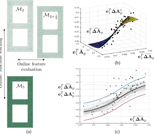
Figure 6.Machine-learning-based error estimation procedure. The overkill error (difference between

the current mesh and a much finer mesh as shown in (a)) is postulated as being an unknown function of an error estimate. The inexpensive error estimate is the distance between the results obtained when using the current mesh and those obtained when using a slightly refined mesh as shown in. (b) The statistical learning is done offline via a Monte-Carlo sampling of the true error (using the prior as sampling density) and the adaptive fitting of a Neural Network regression. The regression is bootstrapped to provide enhanced stability, and derive confidence interval estimates for the overall error estimation procedure which is shown in (c). Both the size of the dataset and the hyperparameters of the network are found automatically via a Greedy process that is not detailed in this paper.

Now, we trainnd+npmultivariate neural network regression models

c ∆Ad(µ) c ∆Ap(µ) ! =                       Rd,1 end 1 T (_A˜_d(µ)−A¯_d(µ)) end 1 T_˜ Ad(µ) ! ,θd,1 ! ... Rd,nd end n_dT(A˜d(µ)−A¯d(µ)) end n_dTA˜d(µ) ! ,θ_d,nd ! Rp,1 en₁pT(_A˜_p(µ)−A¯_p(µ)) en₁pTA˜p(µ) ! ,θp,1 ! ... Rp,np    e np np T (_A˜_p(µ)−A¯_p(µ)) ennpp T ˜ Ap(µ)  ,θp,np                         (34)

Each of the regressionRl,iis a single-hidden layer bootstrap-aggregated neural network model

withnnneurons andnnbsbootstrap replicates.

Rl,i x y ! ,θl,i ! = 1 k nnbs

∑

k=1 nn

∑

j=1 a(k)_j tanha(k)_x,jx+a(k)_y,jy+o(k)_j +o(k) (35) Training

We sample artificial “data” by running the overkill computational modelnmltimes, after sampling

the training set parameters {µml₁ ,µml₂ , ... ,µml_nml} from prior πµ. The number of neurons and the

cardinality of the training set is chosen automatically by making use of an automatised early-stopping methodology that aims to maximise the predictive coefficient of determination. We will not detail this procedure here. Fitting of the nonlinear regression coefficients is performed by employing standard least-squares method, solved by a gradient descent algorithm with randomised initialisation. Outliers of the set of bootstrap replicates are identified and eliminated to decrease the variance of the boostrap-aggregated regression model.

An example of fitted regression model is represented in Figure6, where the output is the

discretisation error in the first free vibration circular frequency (i.e., regression modelRd,1).

5.4. Bootstrap Confidence Intervals for the MCMC Sampler

At any iterationnof the MCMC sampler, a Monte-Carlo estimate of the discretisation error for

the posterior density of the ith component ofµis given by

Dks(n):=Dks(πˆ (n) µi|d(µi), ¯π (n) µi|d(µi)) =sup_µ i (_Πˆ(n) µi|d(µi)− ¯ Π(n) µi|d(µi)) (36) where ¯ Π(n) µi|d=d(µi):= 1 ˜ n n

∑

k=n−n+1˜ I(µi; ¯µk,i ≤µi), (37) and ˆ Π(n) µi|d=d(µi):= 1 ˜ n n

∑

k=n−n+1˜ I(µi; ˆµ_k,i ≤µi). (38)

Crucially, D(n)ks is a random variable whose statistics, and in particular its bias and variance,

strongly depend on the length of the Markov chain. Unfortunately, evaluating the convergence of any statistics provided by MCMC is difficult, due to the statistical dependency between successively drawn samples.

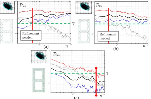
Following standard diagnostic approaches for MCMC samplers (e.g., the Gelman-Rubin

convergence test [53,54]), we will run nc ≥ 10 independent (tempered) MCMC chains in parallel

and pool all the resulting samples, after discarding the first 25% of every individual chain as burn-in

(see Figure7as a visual aid). The pooled samples at iterationnof the multiple-chain MCMC (MC3)

algorithm are ¯ S(n)= nc

∏

i=1 ¯ S_i(n) _Sˆ(n)₌

_∏

nc i=1 ˆ S_i(n) (39)

where ∏denotes the cartesian product. In the previous expression, the sample set from chain i

(at ambient temperature) is ¯

Materials2019,12, 642 16 of 24

D_ks(n)is now the pooled KS distance estimate provided by the MC3algorithm (we will keep the same

notation for the sake of simplicity). Formally, we simply replace Equation (37) by ¯ Π(n) µi|d=d(µi):= 1 nc 1 ˜ n nc

∑

l=1 n

∑

k=n−n+1˜ I(µi; ¯µl,k,i ≤µi), (41)

and perform a similar operation to define the pooled corrected empirical distribution.

The independence of the nc MCMC chains allows us to compute confidence intervals for

Dks(n) by making use of the non-parametric bootstrap. This is done by resampling ¯S(n) and ˆS(n)

with replacement, generating bootstrap replicates of the pooled sample sets {_S¯(n)

k }k∈J1nbsK and {_Sˆ(n) k }k∈J1nbsK, ¯ S_k(n)=

∏

i=∈Bk ¯ S_i(n) _Sˆ(n) k =

∏

i=∈Bk ˆ S_i(n), (42) whereBk∈(J1ncK)

nbs_{is such that each element of this set is drawn uniformly over}

J1ncKandkvaries

between 1 and a large numbernbs, typically set to 1000. For each replicate, statisticsD_ks(n), denoted by

D_ks,k(n), can be computed in a straightforward manner by using the bootstrap replicates of the pooled

empirical distributions ¯ Π(n) µi|d=d,k(µi):= 1 nc 1 ˜ n

∑

¯ µ?_i∈S¯_k(n) I(µi; ¯µ?_i ≤µi), (43) ˆ Π(n) µi|d=d,k(µi):= 1 nc 1 ˜ n

∑

ˆ µ?_i∈Sˆ_k(n) I(µi; ˆµ?_i ≤µi), (44) which reads as Dks,k(n) :=Dks(πˆ (n) µi|d,k(µi), ¯π (n) µi|d,k(µi)) =sup_µ i _(Πˆ(n) µi|d,k(µi)−Π¯ (n) µi|d,k(µi)) , (45)

Finally, the bootstrap confidence intervals are calculated by calculating theXth and(100−X)th

bootstrap percentiles such that theXth percentile reads as

q(n)_X =QX {D(n)_ks,k}k_∈J1n_bsK −median{D(n)_ks,k}k_∈J1n_bsK +D(n)_ks (46)

whereQX is an operator that extracts theXth andYth percentile of the set passed as argument.

It is important to understand that the derived bootstrap confidence interval stands for a chain

of finite lengthn, and not for the asymptotic limit. In fact, estimateD_ks(n)ofDks is strongly biased

(upward for small asymptotic errorsDksand typically downward for large asymptotic errors), which

is due to two factors:

• the existence of the burn-in phase. For smalln, each individual chain will be strongly affected

by the initialisation of the chains. For small asymptotic errors, this can be expected to have a strong upward bias effect providing that the initialisation is disperse, which is often the case in practice (e.g., initialisation from the prior, sequential MC approaches with decreasing levels of

noise). This can be visualised in Figure7. Two incomplete chains running on the same probability

density may be exploring completely different regions of space, yielding values ofDksthat are

large, even in the case where the corrected and uncorrected densities are close to one another.

• the discrete evaluation of the KS distance itself, which generates an additional (upward) bias.

The variance ofD(n)_ks decreases with the number of chains of the MC3_{algorithm (which is not a}

free parameter as overall CPU cost increases linearly withnc). Of course, bias and variance are both