A jackknife and voting classifier approach to feature selection and classification.

UC Davis Previously Published Works

Title

A jackknife and voting classifier approach to feature selection and classification. Permalink https://escholarship.org/uc/item/9q6693x6 Authors Taylor, Sandra L Kim, Kyoungmi Publication Date 2011-04-27 DOI 10.4137/cin.s7111 Peer reviewed

Cancer Informatics 2011:10 133–147 doi: 10.4137/CIN.S7111

This article is available from http://www.la-press.com.

© the author(s), publisher and licensee Libertas Academica Ltd.

This is an open access article. Unrestricted non-commercial use is permitted provided the original work is properly cited.

Open Access

Full open access to this and thousands of other papers at

http://www.la-press.com. M e T h o d o L o g y

A Jackknife and Voting Classifier Approach to Feature

Selection and Classification

Sandra L. Taylor and Kyoungmi Kim

division of Biostatistics, department of Public health Sciences, University of California School of Medicine, davis, CA, USA. Corresponding author email: [email protected]

Abstract: With technological advances now allowing measurement of thousands of genes, proteins and metabolites, researchers are using this information to develop diagnostic and prognostic tests and discern the biological pathways underlying diseases. Often, an

investigator’s objective is to develop a classification rule to predict group membership of unknown samples based on a small set of features and that could ultimately be used in a clinical setting. While common classification methods such as random forest and support vector machines are effective at separating groups, they do not directly translate into a clinically-applicable classification rule based on a small number of features.We present a simple feature selection and classification method for biomarker detection that is intuitively understandable and can be directly extended for application to a clinical setting. We first use a jackknife procedure to identify important features and then, for classification, we use voting classifiers which are simple and easy to implement. We compared our method to random forest and support vector machines using three benchmark cancer ‘omics datasets with different characteristics. We found our jackknife procedure and voting classifier to perform comparably to these two methods in terms of accuracy. Further, the jackknife proce

-dure yielded stable feature sets. Voting classifiers in combination with a robust feature selection method such as our jackknife proce-dure offer an effective, simple and intuitive approach to feature selection and classification with a clear extension to clinical applications. Keywords: classification, voting classifier, gene expression, jackknife, feature selection

Introduction

With technological advances now allowing mea-surement of thousands of genes, proteins and metabolites, researchers are using this information to develop diagnostic and prognostic tests and dis-cern the biological pathways underlying diseases.

Often, researchers initially seek to separate patients

into biologically-relevant groups (e.g., cancer versus control) based on the full suite of gene expression,

protein or metabolite profiles. Commonly though, the

ultimate objective is to identify a small set of features contributing to this separation and to develop a

classi-fication rule to predict group membership of unknown

samples (e.g., differentiate between patients with and without cancer or classify patients according to their

likely response to a treatment).

A number of methods have been developed for

feature selection and classification using gene expres -sion, proteomics or metabolomics data. All methods

share the two essential tasks of selecting features and constructing a classification rule, but differ in how these two tasks are accomplished. Methods can be categorized into three groups: filter, wrapper and

embedded methods based on the relationship between

the feature selection and classification tasks.1 _{In filter}

methods, feature selection and classification are con

-ducted independently. Typically, features are ranked

based on their ability to discriminate between groups using a univariate statistic such as Wilcoxon, t-test, between-group to within-group sum of squares (BSS/

WSS), and an arbitrary number of the top-ranking features are then used in a classifier. For wrapper

methods, the feature selection step occurs in concert

with classifier selection; features are evaluated for a specific classifier and in the context of other features.

Lastly, with embedded techniques feature

selec-tion is fully integrated with classifier construcselec-tion.

Numerous methods within each category have been

developed; Saeys et al1 _{discuss the relative merits and}

weakness of these methods and their applications in

bioinformatics.

Support vector machine (SVM)2 _{and random forest}3 are embedded methods that are two of the leading

fea-ture selection and classification methods commonly used in ‘omics research. Both methods have proved

effective at separating groups using gene expres-sion data4–6 _{and proteomics}7–10 _{and recently SVM} has been applied to metabolomics data.11 _However,

while these methods demonstrate that groups can be differentiated based on gene expression or protein

profiles, their extension to clinical applications is not readily apparent. For clinical applications, classifiers

need to consist of a small number of features and to use a simple, predetermined and validated rule for

prediction. In random forest, the classification rule

is developed by repeatedly growing decision trees

with final sample classification based on the major -ity vote of all trees. Although important features can

be identified based on their relative contribution to classification accuracy, the method does not directly translate into a clinicially-meaningful classification rule. SVM are linear classifiers that seek to find the

optimal (i.e., provides maximum margin) hyperplane separating groups using all measurements and thus

does not accomplish the first task, that of feature

selection. Several methods for identifying important features have been proposed6,12 _{but as with random}

forest, the method does not yield classification rules relevant to a clinical setting. Further, SVM results can

be very sensitive to tuning parameter values.

Voting classifiers are a simple, easy to understand classification strategy. In an unweighted voting clas

-sifier, each feature in the classifier “votes” for an unknown sample’s group membership according to

which group the sample’s feature value is closest. The majority vote wins. Weighted voting can be used to give greater weight to votes of features with stronger evidence for membership in one of the groups. Voting

classifiers have been sporadically used and evaluated

for application to gene expression data.13–16 _Dudoit et al14 _{found Golub’s}13 _{weighted voting classifier per} -formed similarly to or better than several discriminant

analysis methods (Fisher linear, diagonal and linear) and classification and regression tree based predictors,

but slightly poorer than diagonal linear discriminant analysis and k-nearest neighbor. The weighted voting

classifier also performed similarly to SVM and regu -larized least squares in Ancona et al15 _{study of gene} expression from colon cancer tumors. These results

suggest that voting classifiers can yield comparable results to other classifiers.

To be clinically-applicable, classification rules need

to consist of a small number of features that will con-sistently and accurately predict group membership. Identifying a set of discriminatory features that is

training set is important for developing a broadly

applicable classifier. In the traditional approach to classifier development, the data set is separated into a training set for classifier construction and a test set(s) for assessment of classifier performance. Using the training set, features are ranked according to some

criterion and the top m features selected for inclusion

in the classifier applied to the test set. By repeatedly

separating the data into different training and test

sets, Michelis et al17 _{showed that the features}

identi-fied as predictors were unstable, varying considerably with the samples included in the training set. Baek

et al18 _{compared feature set stability and classifier} performance when features were selected using the traditional approach versus a frequency approach. In a frequency approach, the training set is repeatedly

separated into training and test sets; feature selec

-tion and classifier development is conducted for each training set. A final list of predictive features is gener -ated based on the frequency occurrence of features

in the classifiers across all training:test pairs. They

showed that frequency methods for identifying pre-dictive features generated more stable feature sets

and yielded classifiers with accuracies comparable

to those constructed with traditional feature selection approaches.

Here we present a simple feature selection and

classification method for biomarker detection that

is intuitively understandable and can be directly extended for application to a clinical setting. We

first use a jackknife procedure to identify impor -tant features based on a frequency approach. Then

for classification, we use weighted or unweighted voting classifiers. We evaluate the performance of voting classifiers with varying numbers of features using leave-one-out cross validation (LOOCV) and multiple random validation (MRV). Three cancer ‘omics datasets with different characteristics are

used for comparative study. We show our approach

achieves classification accuracy comparable to ran

-dom forest and SVM while yielding classifiers with

clear clinical applicability.

Methods

Voting classifiers and feature selection

The simplest voting classifier is an unweighted classi

-fier in which each feature “votes” for the group mem

-bership of an unknown sample according to which

group mean the sample is closest. Let x_j(g) be the value of feature g in test sample j and consider two groups (0, 1). The vote of feature g for sample j is

v g if x g x g g if x g g x g j j j j j ( ) | ( ) ( ) | | ( ) ( ) | | ( ) ( ) | | ( = − < − − < 1 0 1 0 0 µ µ µ g ))− ( ) |     µ1 g (1) where µ₁(g) and µ₀(g) are the means of feature g

in the training set for group 1 and 0, respectively.

Combining the votes of all features in the classifier

(G), the predicted group membership (C_j) of sample j

is determined by C if I v g I v g if I v g I v g j G G G G = 1 1 0 0 0 1 ( ) [ ( ) ] ( ) [ ( ) ] =

[

]

[

]

∑

∑

∑

∑

The unweighted voting classifier gives “equal”

weight to all votes with no consideration of differences in the strength of the evidence for a

classification vote by each feature. Alternatively,

various methods for weighting votes are available.

Mac Donald et al16 _{weighted votes according to the} deviation of each feature from the mean of the two classes, ie, W g_j( )= x g_j( ) [ ( )− µ₁ g +µ₀( ) / ]g 2 . This approach gives greater weight to features with values farther from the overall mean and thus more strongly suggesting membership in one group. However, if

features in the classifier have substantially different

average values, this weighting strategy will dispro-portionately favor features with large average values. Golub et al13 _{proposed weighting each feature’s} vote according to the feature’s signal-to-noise ratio

a_g= [µ₁(g) -µ₂(g)]/[σ₁(g) +σ₂(g)]. In this approach, greater weight is given to features that best discrimi-nate between the groups in the training set. While addressing differences in scale, this weighting strat-egy does not exploit information in the deviation of

the test sample’s value from the mean as MacDonald

et al’s16 _{method does.}

We propose a novel weighted voting classifier that

accounts for differences among features in terms of variance and mean values and incorporates the mag-nitude of a test sample’s deviation from the overall feature mean. In our weighting approach, the vote of

feature g is weighted according to the strength of the

evidence this feature provides for the classification of

sample j, specifically. w g x g g g x g g g n j j i i ( ) ( ) ( ) ( ) ( ) ( ) ( ) = − +     − +     µ µ µ µ 1 0 2 1 0 2 2 2 ==

∑

where w_j(g) is the weight of feature g for test set sam-ple j, x_j(g) is the value of feature g for test sample j,

x_i(g) is the value of feature g for training sample i, n

is the number of samples in the training set, and µ₁(g) and µ₀(g) are the grand means of feature g in the train-ing set for group 1 and 0, respectively. This approach weights a feature’s vote according to how far the test set sample’s value is from the grand mean of the

train-ing set like MacDonalds et al’s16 _{but scales it} accord-ing the feature’s variance to account for differences in magnitude of feature values. Test set samples are

classified based on the sum of the weighted votes of

each feature.

We used a jackknife procedure to select and rank features to include in the classifier (G = {1, 2, … , g, … , m}, where m,,n = number of all features in

dataset). For this approach, data are separated into a training and test set. Using only the training set,

each sample is sequentially removed and features are

ranked based on the absolute value of the t-statistic calculated with the remaining samples. We then

retained the top ranked 1% and 5% of features for each jackknife iteration. This step yielded a list of the most discriminating features for each jackknife iteration. Then the retained features were ranked

according to their frequency occurrence across the

jackknife iterations. Features with the same fre

-quency of occurrence were further ranked accord -ing to the absolute value of their t-statistics. Using the frequency ranked list of features, we constructed voting classifiers with the top m most frequently

occurring features (fixed up to m= 51 features in this

study), adding features to the classifier in decreasing

order of their frequency of occurrence and applied

the classifier to the corresponding test set. In both the LOOCV and MRV procedures, we used this jackknife procedure to build and test classifiers; thus

feature selection and classifier development occurred

completely independently of the test set.

For clarification, our two-phase procedure is

described by the following sequence:

Phase 1: Feature selection via jackknife and voting classifier construction

For each training:test set partition,

1. Select the m most frequently occurring features

across the jackknife iterations using the training set for inclusion in the classifier (G), where G is the set of the m most frequently occurring features in descending order of frequency.

2. For each feature g selected in step 1, calculate the vote of feature g for test sample j using equation (1).

3. Repeat step 2 for all features in the classifier G.

4. Combine the votes of all features from step 3 and

determine the group membership (C_j) of sample j using equation (2). For the weighted voting classi

-fier, the vote of feature g is weighted according to equation (3).

5. Repeat steps 2–4 for all test samples in the

test set.

Phase 2: Cross-validation

6. Repeat for all training:test set partitions.

7. Calculate the misclassification error rate to assess performance of the classifier.

data sets

We used the following three publicly available data sets to evaluate our method and compare it to random forest and support vector machines.

Leukemia data set

This data set from Golub et al13 _{consists of gene} expression levels for 3,051 genes from 38 patients,

11 with acute myeloid leukemia and 27 with acute lymphoblastic leukemia. An independent validation set was not available for this data set. The classifica -tion problem for this data set consists of

distinguish-ing patients with acute myeloid leukemia from those with acute lymphoblastic leukemia.

Lung cancer data set

This data set from Gordon et al19 _{consists of} expres-sion levels of 12,533 genes in 181 tissue samples from patients with malignant pleural mesothelioma

(31 samples) or adenocarcinoma (150 samples) of the lung. We randomly selected 32 samples, 16 from each group to create a learning set. The remaining 149 samples were used as an indepen-dent validation set. It was downloaded from http://

datam.i2r.a-star.edu.sg/datasets/krbd/LungCancer/ LungCancer- Harvard2.html.

Prostate cancer data set

Unlike the leukemia and lung cancer data sets, the

prostate cancer data set is proteomics data set con-sisting of surface-enhanced laser desorption

ioniza-tion time-of-flight (SELDI-TOF) mass spectrometry

intensities of 15,154 proteins.20 _{Data are available} for 322 patients (253 controls and 69 with pros-tate cancer). We randomly selected 60 patients (30 controls and 30 cancer patients) to create a learn-ing set and an independent validation set with 262 patients (223 controls and 39 cancer patients). The data were downloaded from http://home.ccr.cancer. gov/ncifdaproteomics/ppatterns.asp.

Performance assessment

To evaluate the performance of the voting classifiers, we used LOOCV and MRV. For MRV, we randomly

partitioned each data set into training and test sets at a

fixed ratio of 60:40 while maintaining the group dis -tribution of the full data set. We generated 1,000 of

these training:test set pairs. For each training:test set

pair, we conducted feature selection and constructed

classifiers using the training set and applied the clas

-sifier to the corresponding test set.

We compared the voting classifiers to random

forest and support vector machines. The random forest

procedure was implemented using the randomForest package version 4.5-3421 _{for R.}22 _{Default values of}

the randomForest function were used. Support vec -tor machines were generated using the svm function

in the package e1071.23 _{A radial kernel was assumed} and 10-fold cross validation using only the training set was used to tune gamma and cost parameters for each training:test set pair. Gamma values rang-ing from 0.0001 to 2 and cost values of 1 to 20 were

evaluated. As with the voting classifiers, random for

-est and SVM classifiers were developed using the

training set of each training:test set pair within the

LOOCV and MRV strategies and using features iden

-tified through the jackknife procedure rather than all

features, ie, for a training:test set pair, all features that

occurred in the top 1% or 5% of the features across the jackknife iterations were used in developing the classifiers.

Application to independent

validation sets

The lung and prostate cancer data sets were large

enough to create independent validation sets. For

these data sets, we used the training sets to develop

classifiers to apply to these sets. To identify fea

-tures to include in the voting classifiers, we identi

-fied the m most frequently occurring features for each training:test set pair, with m equal to odd numbers

from three to 51. For each m number of features, we

ranked the features according to their frequency of occurrence across all the jackknife samples. Voting classifiers with three to 51 features were constructed

using all of the training set samples and applied to

the independent validation sets. Random forest and SVM classifiers were constructed using any feature

that occurred at least once in the feature sets

iden-tified through the jackknife strategy procedure. We constructed classifiers using the top 1% and 5% fea

-tures identified through the jackknife procedure for both validation strategies (LOOCV and MRV).

Results

Performance evaluation and comparison

with random forest and support vector

machines

We evaluated our method and compared it to random

forest and SVM through application to three

well-studied data sets from cancer studies (Table 1). Two of

these data sets (leukemia13 _{and lung cancer)}19 _consist

of gene expression data; the third (prostate cancer)20 is proteomics data. We evaluated accuracy of the

vot-ing classifiers for each data set usvot-ing the top 1% and 5% of features of the jackknife training sets for two validation strategies—LOOCV, and MRV using 1,000

randomly generated training:test set pairs.

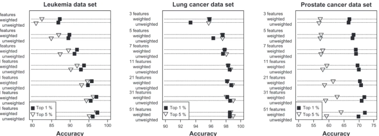
Accuracy of the two voting classifiers increased

with the number of features included in the

classi-fier (Figs. 1 and 2). However, the largest

improvem-ents in accuracy occurred as the number of features increased from 3 to about 11 after which further

increases were small. In fact, accuracies within 5% of

than 13 features. The feature selection step influenced accuracy of the voting classifiers more strongly than the number of features included in the classifier. For both weighted and unweighted voting classifiers, accuracy was usually higher when the classifier was constructed based on the top 1% of features rather than the top 5% (Figs. 1 and 2), suggesting that a classifier with a small number of features could be developed. The weighted voting classifier generally

yielded higher accuracy than the unweighted voting

classifier; however, the differences tended to be small, within a few percentage points (Figs. 1 and 2).

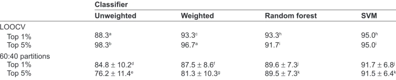
The voting classifiers performed similarly to ran

-dom forest and SVM but classifier performance var -ied considerably for the three data sets evaluated (Fig. 3). All classifier methods performed well for

the lung cancer data set with mean accuracies greater

than 95%. Both the weighted and unweighted voting classifiers achieved greater than 90% accuracy with only three features and greater than 98% accuracy with only nine features. SVM yielded a relatively low

accuracy based on the top 5% of features for the lung cancer data set (84.6%); accuracy potentially could

be improved with more extensive parameter tuning.

Classifier accuracy also was high for the leukemia data set with all classifiers achieving over 95% accuracy. The voting classifiers performed slightly better than random forest for this data set; SVM had the high

-est accuracy when the top 5% of features were used to construct the classifier. In contrast, for the pros

-tate cancer data set, classifier accuracy was consider -ably lower and more variable than for the other data

sets. Accuracy ranged from a low of 56.5% for SVM under MRV using the top 5% of features to a high of 83.3% for SVM using the top 1% in LOOCV. In

general, though, random forest tended to produce the

highest accuracies with the voting classifiers yielding

intermediate performances.

The poor performance of all classifiers for the

prostate data set suggested greater heterogeneity in

one of the groups. Control samples in this data set

consisted of patients with normal prostates as well as

Table 1. Characteristics of data sets.

Data set Ref Data type # features Training set Independent

validation set

# cases # control

Leukemia 13 gene expression 3,051 11a _{27 No}

Lung cancer 19 gene expression 12,533 16 16 149 (15 controls,

134 cases) Prostate

cancer 20 Proteomics 15,154 30 30 262 (223 controls, 39 cases

note:a_{Patients with acute myeloid leukemia were considered “cases” and those with acute lymphoblastic leukemia were used as “controls”.}

3 features weighted unweighted 5 features weighted unweighted 7 features weighted unweighted 11 features weighted unweighted 21 features weighted unweighted 31 features weighted unweighted 51 features weighted unweighted 3 features weighted unweighted 5 features weighted unweighted 11 features weighted unweighted 7 features weighted unweighted 21 features weighted unweighted 31 features weighted unweighted 51 features weighted unweighted 3 features weighted unweighted 5 features weighted unweighted 11 features weighted unweighted 7 features weighted unweighted 21 features weighted unweighted 31 features weighted unweighted 51 features weighted unweighted 80 85 90 95 100 90 92 94 96 98 100 50 55 60 65 70 75 Top 1 % Top 5 % Top 1 % Top 5 % Top 1 % Top 5 % Accuracy Lung cancer data set

Leukemia data set Prostate cancer data set

Accuracy Accuracy

Figure 1. Multiplerandom validation results for voting classifiers. Mean accuracy for voting classifiers (unweighted and weighted) with varying numbers of

features included in the classifier based on 1,000 random training:test set partitions of two gene expression data sets (leukemia, lung cancer) and a pro

-teomics data set (prostate cancer). Features to include in the classifiers were identified through a jackknife procedure through which features were ranked according to their frequency of occurrence in the top 1% or 5% most significant features based on t-statistics across all jackknife samples.

patients with benign prostate hyperplasia (BPH). In Petricoin et al’s original analysis,20 _{26% of the men}

with BPH were classified as having cancer. They noted that some of these apparent misclassifications actually could be correct because over 20% of sub

-jects identified as not having cancer based on an

initial biopsy were later determined to have cancer.

Thus, the poorer classification performance for the

prostate data set could result from BPH patients having incorrectly been considered controls which led to increased within-group variation relative to between-groups variation. 100 95 90 90 91 92 93 94 95 96 97 98 99 100 85 85 80 75 70 65 60 55 50 80 75 Number of features

Leukemia data set Lung cancer data set Prostate cancer data set

Number of features Number of features

Accuracy 3 7 11 15 19 23 27 31 35 39 43 47 51 3 7 11 15 19 23 27 31 35 39 43 47 51 3 7 11 15 19 23 27 31 35 39 43 47 51 Unweighted top 1% Unweighted top 5% Weighted top 1% Weighted top 5% Unweighted top 1% Unweighted top 5% Weighted top 1% Weighted top 5% Unweighted top 1% Unweighted top 5% Weighted top 1% Weighted top 5%

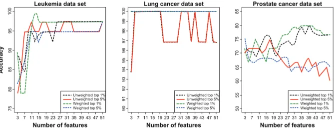
Figure 2. Leave-one-outcross validation (LOOCV) results for voting classifiers. Accuracy for voting classifiers (unweighted and weighted) with varying

numbers of features included in the classifier based on LOOCV of two gene expression data sets (leukemia, lung cancer) and a proteomics data set (prostate cancer). Features to include in the classifiers were identified through a jackknife procedure through which features were ranked according to their frequency of occurrence in the top 1% or 5% most significant features based on t-statistics across all jackknife samples.

10 0 95 90 85 10 0 10 0 90 80 70 60 50 40 95 90 85 80

Unwgt Wgt RF SVM Unwgt Wgt RF SVM Unwgt Wgt RF SVM Unwgt Wgt RF SVM Unwgt Wgt RF SVM Unwgt Wgt RF SVM

Classifiers Classifiers Classifiers

Prostate cancer data set Lung cancer data set

Leukemia data set

Accurac

y

Top 1% Top 5% Top 1% Top 5% Top 1% Top 5%

Figure 3. Comparison of voting classifiers, random forest and SVM. Accuracy (mean ± SE) for unweighted (Unwgt) and weighted (Wgt) voting classifiers,

random forest (RF) and support vector machines (SVM) based on 1,000 random training:test set partitions of two gene expression data sets (leukemia,

lung cancer) and a proteomics data set (prostate cancer). Features to include in the classifiers were identified through a jackknife procedure through

which features were ranked according to their frequency of occurrence in the top 1% or 5% most significant features based on t-statistics across all

jackknife samples. Horizontal bars show LOOCV results. Results presented for weighted and unweighted voting classifiers are based on the number of features yielding the highest mean accuracy. For the leukemia data set the 49 or 51 features yielded the highest accuracy for the voting classifiers in the MRV procedure while for LOOCV, the best numbers of features for the unweighted voting classifier were 17 and 11 using the top 1% and 5% of features, respectively and were 13 and 51, respectively for the weighted voting classifier. For the lung cancer data set, 3 and 5 features were best with LOOCV for the weighted and unweighted classifier. Under MRV, 51 features yielded the highest accuracy for the weighted voting classifier while 19 or 39 features needed for the unweighted voting classifier based on the top 1% and 5% of features, respectively. With the prostate cancer data set, the unweighted voting classifier used 31 and 49 features with MRV and 35 and 17 features with LOOCV based on the top 1% and 5% of features, respectively. For the weighted voting classifier, these numbers were 49, 51, 31 and 3, respectively. The number of features used in random forest and SVM varied across the training:test set partitions. Depending on the validation strategy and percentage of features retained in the jackknife procedure, the number of features ranged from 67

features could easily form the basis of a diagnostic test for clinical application consisting of the mean and variances of these features in a large sample of patients with adenocarcinoma and mesothelioma.

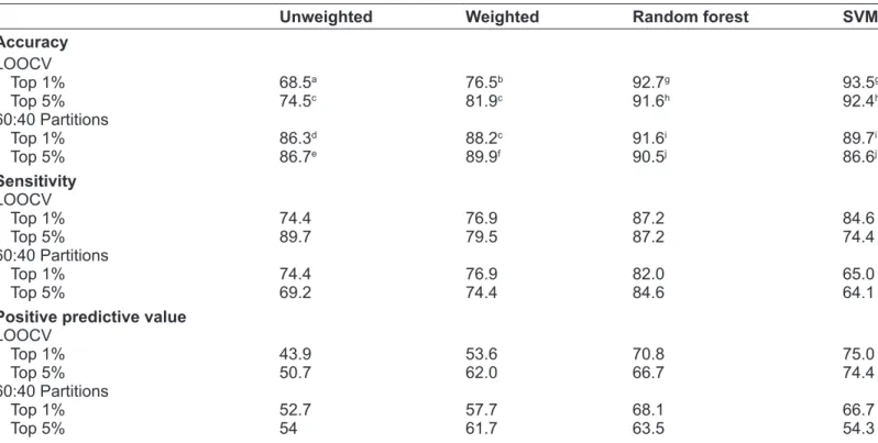
Classifier performance was quite variable when

applied to the prostate cancer validation data set. Accuracy was generally highest for the random forest

classifier (Table 4). When features to use in the

clas-sifier were derived from the LOOCV procedure, the voting classifiers had relatively low accuracy (68.5% to 76.5%) while SVM and random forest had accura

-cies greater than 90%. Accuracy of the voting classi

-fiers improved when features were derived through MRV and were within 5% of random forest and SVM. Sensitivity and positive predictive value were

highest with random forest and similar between the

voting classifiers and SVM. As seen in the LOOCV and MRV analyses, the performance of all classifiers

increased when BPH samples were excluded from the control group. When applied to the independent

validation set, the weighted voting classifier achieved accuracies of 93% to 99%; random forest and SVM were similar with accuracies of 97% to 99% and 89% to 99%, respectively.

Data set variability and classifier

performance

Classifier performance varied considerably among the three data sets. Accuracy was high for the leuke -mia and lung cancer data sets but lower for the

pros-tate cancer data set. These differences likely reflect

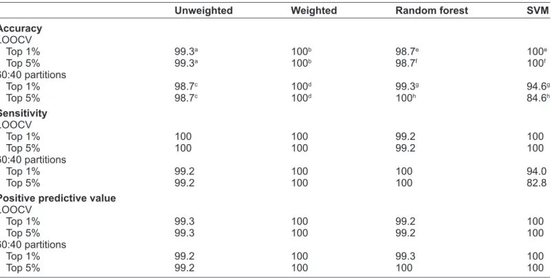
Table 2. Accuracy of classifiers applied to prostate cancer data set excluding benign prostate hyperplasia samples.

Classifier

Unweighted Weighted Random forest sVM

LooCV Top 1% 88.3a _93.3c _93.3h _95.0h Top 5% 98.3b _96.7a _91.7i _95.0i 60:40 partitions Top 1% 84.8 ± 10.2d _{87.5 ± 8.6}f _{89.6 ± 7.3}j _{91.7 ± 6.8}j Top 5% 76.2 ± 11.4e _{81.3 ± 10.3}g _{89.5 ± 7.3}k _{91.5 ± 6.4}k

notes: Accuracy of voting classifiers (unweighted and weighted), random forest and SVM applied to the prostate cancer data set excluding benign prostate hyperplasia samples from the control group. Features to include in the classifiers were derived using the top 1% or 5% of features based on t-statistics through a jackknife procedure using training sets in leave-one-out cross validation (LOOCV) or multiple random validation (60:40 partitions).

Mean ± Sd accuracy reported for 1,000 60:40 random partitions. a_{Highest accuracy achieved with 7 features in classifier;} b_{highest accuracy achieved}

with 9 features in classifier; c_{Highest accuracy achieved with 13 features in classifier;} d_{Highest accuracy achieved with 21 features in classifier;} e_highest

accuracy achieved with 47 features in classifier; f_{Highest accuracy achieved with 23 features in classifier,} g_{highest accuracy achieved with 51 features}

in classifier. The number of features used in random forest and SVM varied across the training:test set partitions. The ranges were: h_{265–340 features;} i_{1,194–1,268 features;} j_212–533; k_{1,412–1,970 features.}

We further analyzed the prostate cancer data set excluding BPH patients from the control group. The

performance of all classifiers increased markedly with exclusion of BPH patients. For the LOOCV and MRV procedures, random forest and SVM achieved accuracies of 90% to 95% and the accuracy of the voting classifiers ranged from 76% to 98%. These values were 10% to 20% greater than with inclusion

of the BPH samples (Table 2).

Independent validation set evaluation

In cases where data sets are too small, overfitting can

be a severe issue when assessing a large number of features. Therefore, it is very important to evaluate the

accuracy of classifier performance with an independent

validation set of samples that are not part of the

devel-opment of a classifier. Hence, we constructed voting, random forest and SVM classifiers using only the train -ing sets and applied them to independent validation sets from the lung cancer and prostate cancer data sets.

All classifiers had very high accuracies when

applied to the lung cancer data set (Table 3). Sensitivity

and the positive predictive value of the classifiers also were very high, 99% to 100%. The one exception was SVM with features selected through MRV which

had considerably lower accuracies and sensitivities.

The weighted voting classifier had 100% accuracy

using 49 features. However, with just three features (37205_at, 38482_at and 32046_at), the unweighted

voting classifiers had greater than 90% accuracy and the weighted more than 93% accuracy. These three

Table 3. Performance of classifiers applied to independent validation set of lung cancer data set.

Unweighted Weighted Random forest sVM

Accuracy LooCV Top 1% 99.3a ₁₀₀b _98.7e ₁₀₀e Top 5% 99.3a ₁₀₀b _98.7f ₁₀₀f 60:40 partitions Top 1% 98.7c ₁₀₀d _99.3g _94.6g Top 5% 98.7c ₁₀₀d ₁₀₀h _84.6h sensitivity LooCV Top 1% 100 100 99.2 100 Top 5% 100 100 99.2 100 60:40 partitions Top 1% 99.2 100 100 94.0 Top 5% 99.2 100 100 82.8

Positive predictive value

LooCV Top 1% 99.3 100 99.2 100 Top 5% 99.3 100 99.2 100 60:40 partitions Top 1% 99.2 100 99.3 100 Top 5% 99.2 100 100 100

notes: Accuracy, sensitivity, and positive predictive value of voting classifiers (unweighted and weighted), random forest and SVM applied to independent data sets from the lung cancer data set. Features to include in the classifiers were derived using the top 1% or 5% of features based on t-statistics

through a jackknife procedure using training sets in leave-one-out cross validation (LOOCV) or multiple random validation (60:40 partitions). a_highest

accuracy achieved with 37 features in classifier; b_{Highest accuracy achieved with 23 features in classifier;} c_{highest accuracy achieved with 15 features in}

classifier; d_{Highest accuracy achieved with 49 features in classifier. The number of features used in developing SVM and random forest classifiers were:} e_{452 features;} f_{1,791 features;} g_{4,172 features;} h_{9,628 features.}

differences in the “signal-to-noise” ratio of features

in these data sets. We used BSS/WSS to characterize

the “signal-to-noise” ratio of each data set and investi

-gated classifier performance in relation to BSS/WSS. First, we calculated BSS/WSS for each feature using all samples of the leukemia data set, and all learning

set samples for the prostate and lung cancer data sets.

Classifier accuracy was highest for the lung cancer data

set and this data had the feature with the highest BSS/

WSS of 3.50. Classifier accuracy was also high for the leukemia data set although slightly lower than for

the lung cancer data set and accordingly the maximum BSS/WSS of features in this data set was smaller at

2.92. Finally, the maximum BSS/WSS for any feature

in the prostate cancer data set was less than 1 (0.98)

and classifier accuracy was lowest for this data set. The “signal-to-noise” ratio of features in the clas

-sifier can also explain the better performance of clas

-sifiers constructed with the top 1% of the features as compared to the top 5%. For the prostate cancer and leukemia training sets, the mean BSS/WSS of features

in the voting classifiers was always higher when the features were derived based on the top 1% than the top 5% (Fig. 4). By considering the top 5% of fea

-tures for inclusion in the classifier, more noise was

introduced and the predictive capability of the

clas-sifiers was reduced. SVM and random forest showed

this effect as well (Fig. 3).

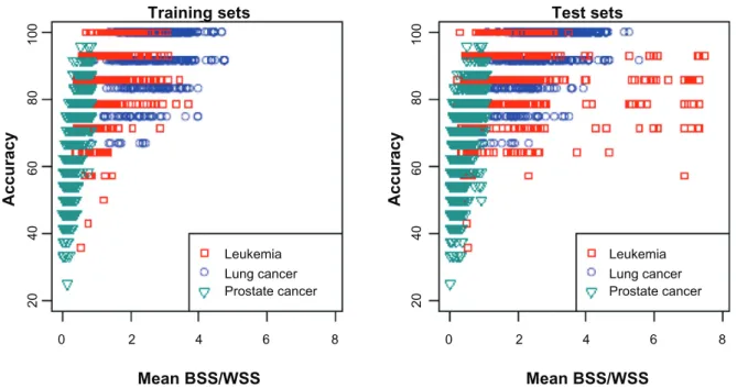
We further evaluated the relationship between

classifier performance and the BSS/WSS of features in the classifier using the weighted voting classifier with just the first three features in order of frequency of occurrence in MRV repetitions. Three features accounted for much of the classifier’s performance particularly for the lung cancer and leukemia data

sets. Accuracy generally increased as the mean BSS/

WSS of the three features included in the classifier

increased in the training and test sets (Fig. 5). The

lung cancer and leukemia data sets had the highest

mean BSS/WSS values and also the highest accura-cies while the lowest BSS/WSS values and accuraaccura-cies

the test sets, when the mean BSS/WSS of these three features was greater than 1, the mean accuracy of the

weighted vote classifier was greater than 80% for all data sets (Leukemia: 89%, Lung Cancer: 95%, Pros

-tate Cancer: 81%) and was considerably lower when the mean BSS/WSS was less than 1 (Leukemia: 82%, Lung Cancer: 80%, Prostate Cancer: 66%).

Interestingly, accuracy was less than 70% for some partitions of the leukemia despite relatively high mean

BSS/WSS values (.3) in the test set. These partitions tended to have one feature with a very high BSS/

WSS (.10) resulting in a large mean BSS/WSS even

though the other features had low values. Further,

for these partitions, the mean values of the features in the test set for each group, particularly those with low BSS/WSS values, tended to be intermediate to those in the training set, resulting in ambiguous

clas-sification for some samples. Thus, even though the

test set features of some partitions had a high mean

BSS/WSS, the classification rule developed from the

training set was not optimal. Overall, the results show

Table 4. Performance of classifiers applied to independent validation set of prostate cancer data set.

Unweighted Weighted Random forest sVM

Accuracy LooCV Top 1% 68.5a _76.5b _92.7g _93.5g Top 5% 74.5c _81.9c _91.6h _92.4h 60:40 Partitions Top 1% 86.3d _88.2c _91.6i _89.7i Top 5% 86.7e _89.9f _90.5j _86.6j sensitivity LooCV Top 1% 74.4 76.9 87.2 84.6 Top 5% 89.7 79.5 87.2 74.4 60:40 Partitions Top 1% 74.4 76.9 82.0 65.0 Top 5% 69.2 74.4 84.6 64.1

Positive predictive value

LooCV Top 1% 43.9 53.6 70.8 75.0 Top 5% 50.7 62.0 66.7 74.4 60:40 Partitions Top 1% 52.7 57.7 68.1 66.7 Top 5% 54 61.7 63.5 54.3

notes: Accuracy, sensitivity, and positive predictive value of voting classifiers (unweighted and weighted), random forest and SVM applied to independent data sets from the prostate cancer data set. Features to include in the classifiers were derived using the top 1% or 5% of features based on t-statistics through a jackknife procedure using training sets in leave-one-out cross validation (LOOCV) or multiple random validation (60:40 partitions). a_highest

accuracy achieved with 37 features in classifier; b_{Highest accuracy achieved with 43 features in classifier;} c_{highest accuracy achieved with 45 features in}

classifier, d_{Highest accuracy achieved with 49 features in classifier;} e_{Highest accuracy achieved with 47 features in classifier;} f_{highest accuracy achieved}

with 27 features in classifier. The number of features used in developing SVM and random forest classifiers were: g_{685 features;} h_{2,553 features;} i_9,890

features; j_{14,843 features.} 1.5 1.0 0.5 0.0 10 20 30 40 50

Number of features in classifier

Mean BSS/WSS

Leukemla 1 % Prostate cancer 1% Prostate cancer 5% Leukemla 5 %

Figure 4. MeanBSS/WSS of features in voting classifiers. Mean BSS/

WSS of features included in the voting classifiers constructed from vary -ing numbers of features for the leukemia and prostate cancer data sets. Mean values were calculated using the training sets from 1,000 random

training: test set partitions. Features to include in the classifiers were iden

-tified through a jackknife procedure through which features were ranked

according to their frequency of occurrence in the top 1% or 5% most

100 80 60 40 20 100 80 60 40 20 0 2 4 6 8 0 2 4 6 8 Accurac y Accurac y Mean BSS/WSS Mean BSS/WSS

Training sets Test sets

Leukemia Lung cancer Prostate cancer Leukemia Lung cancer Prostate cancer

Figure 5. Meanaccuracy of weigthed voting classifier versus mean BSS/WSS. Mean accuracy of the weighted voting classifier using three features versus

the mean BSS/WSS of these features for two gene expression data sets (leukemia, lung cancer) and a proteomics data set (prostate cancer). Mean values

were calculated across 1,000 random training:test set partitions. Features to include in the classifiers were identified through a jackknife procedure through which features were ranked according to their frequency of occurrence in the top 1% most significant features based on t-statistics across all jackknife

samples. Mean BSS/WSS was calculated separately using the training and test set portions of each random partition. that classification accuracy increases as the

“signal-to-noise” ratio increases but even for data sets with

a strong signal, some partitions of the data can yield

low classification accuracies because of random vari -ation in the training and test sets.

Feature frequency

An underlying goal of feature selection and classifi

-cation methods is to identify a small, but sufficient, number of features that provide good classification with high sensitivity and specificity. Our jackknife

procedure in combination with a validation

strat-egy naturally yields a ranked list of discriminatory features. For each training:test set pair, features are ranked by their frequency of occurrence across the jackknife samples and the m most frequently

occur-ring features used to build the classifier for that training:test set pair. Features used in the classifier

for each training:test set pair can be pooled across

all training:test set pairs and features ranked accord

-ing to how frequently they occurred in classifiers.

The features that occur most frequently will be the most stable and consistent features for discriminating between groups.

We compared the frequency of occurrence of

features in the top 1% and 5% of features for the

LOOCV and MRV validation strategies. LOOCV did not provide as clear of feature ranking as MRV. With LOOCV, many features occurred in the top per -centages for all training:test set pairs, and thus were

equally ranked in terms of frequency of occurrence.

In contrast, few features occurred in the top

percent-ages for all 1,000 training:test set pairs with MRV and thus, this procedure provided clearer rankings. Using the more liberal threshold of the top 5% resulted in

more features occurring among the top candidates. As a result, more features were represented in the list of features compiled across the 1,000 training:test set

pairs and their frequencies were lower. For example, for the leukemia data set, 31 features occurred in the top 5% of all 1,000 training:test set pairs while only two occurred in the top 1% of every pair.

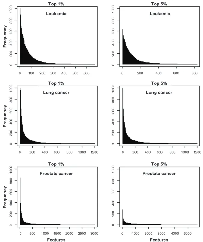
The frequency distributions of the features in the

voting classifiers generated in the MRV strategy was indicative of the performance of the classifier for each data set. Considering the voting classifiers with

51 features, we tallied the frequency that each feature

occurred in the classifier across the 1,000 training:test set pairs. All classifiers performed well for the lung cancer data set; the frequency distribution for this data

set showed a small number of features occurring in

1000 800 600 400 200 0 1000 800 600 400 200 0 1000 800 600 40 0 200 0 1000 800 600 400 200 0 1000 800 600 40 0 200 0 1000 800 600 400 200 0 0 100 200 300 400 500 600 0 200 400 600 800 0 0 500 1000 1500 2000 2500 3000 0 1000 2000 3000 4000 5000 200 400 600 800 1000 1200 0 200 400 600 800 1000 1200 Features Features Top 5% Top 1% Top 5% Top 1% Top 5% Top 1% Prostate cancer Lung cancer Leukemia Frequency Frequency Frequency Leukemia Lung cancer Prostate cancer

Figure 6. Frequencyof occurrence of features in voting classifiers. Frequency of occurrence of features used in voting classifiers containing 51 features

across 1,000 random training: test set partitions of two gene expression data sets (leukemia, lung cancer) and a proteomics data set (prostate cancer).

Features to include in the classifiers were identified through a jackknife procedure through which features were ranked according to their frequency of occurrence in the top 1% or 5% most significant features based on t-statistics across all jackknife samples.

had the next best classification accuracy. With the top 1% of features, this data set showed a small number of features occurring in every partition like the lung cancer data set but with using the top 5% of features, none of the features in the leukemia data set occurred

in all partitions. In fact, the most frequently occur-ring feature occurred in only 600 of the training:test

set pairs. Accordingly, classifier accuracy for the leu

-kemia data set was lower using the top 5% features as compared to the top 1%. Finally, the prostate data

set had the poorest classification accuracy and the

frequency distribution of features differed

substan-tially from the lung cancer and leukemia data sets.

None of the features occurred in all random partitions

and with a 5% threshold, the most frequently occur

-ring features occurred in the classifier in only about

300 of the training:test set partitions. The best

perfor-mance for the voting classifiers occurred when there

were a small number of features that occurred in a

large number of the classifiers constructed for each of

the training:test set pairs.

The instability of the most frequently occurring features for the prostate cancer data set could result in part from the BPH patients. While each training:test set partition had the same number of control and cancer patients, the relative number of BPH patients varied among partitions. Because of the variability within this group, the top features would be expected to be more variable across partitions than for the other data sets.

Discussion

In this study, we showed that voting classifiers per

-formed comparably to random forest and SVM and in some cases performed better. For the three data sets we investigated, the voting classifier method yielded a

small number of features that were similarly effective at classifying test set samples as random forest and

SVM using a larger number of features. In addition to using a small set of features, voting classifiers offer some other distinct advantages. First, they accom

-plish the two essential tasks of selecting a small num

-ber of features and constructing a classification rule.

Second, they are simple and intuitive, and hence they are easily adaptable by the clinical community. Third,

there is a clear link between development of a voting classifier and potential application as a clinical test. In

contrast, clinicians may not understand random forest

and SVM such that the significance and applicability

of results based on these methods may not be apparent.

Further, demonstrating that these methods can accu -rately separate groups in an experimental setting does not clearly translate into a diagnostic test.

We used a frequency approach to identify

impor-tant, discriminatory features at two levels. First, for each training:test set pair, we used a jackknife pro -cedure to identify features to include in the

classi-fier according to their frequency of occurrence. For

the prostate and lung cancer data sets which had an independent validation set, we then selected features

that occurred most frequently in classifiers to con

-struct the final classifier applied to the independent validation set. The results from MRV were better for this step than LOOCV because the feature rankings were clearer under MRV. With LOOCV many features occurred in all classifiers and hence many features had the same frequency rank. In contrast, for MRV few features occurred in the classifiers of every random partition, resulting in a clearer ranking of features.

Our approach for feature selection differs from a

standard LOOCV strategy in that we use a jackknife at each step in the LOOCV to build and test a clas

-sifier such that feature selection occurred completely independently of the test set. Baek et al18 _followed a similar strategy but used V—fold cross validation

rather than a jackknife with the training set to iden -tify important features based on their frequency of

occurrence. Efron24 _{showed that V—fold cross} vali-dation has larger variability as compared to bootstrap methods, especially when a training set is very small.

Because the jackknife is an approximation to the bootstrap, we elected to use a jackknife procedure in

an attempt to identify stable feature sets.

In the jackknife procedure, we ranked features

according the absolute value of t-statistics and

retained the top 1% and 5% of features. Many other ranking methods have been used including BSS/

WSS, Wilcoxon test, and correlation and our method easily adapts to other measures. Popovici et al25

compared five features selection methods including t statistics, absolute difference of means and BSS/

WSS and showed that classifier performance was similar for all feature-ranking methods. Thus, our feature selection and voting classifier method would be expected to perform similarly with other ranking methods. Of significance in our study was the per

-formance differences between classifiers developed based on the top 1% and 5% of features. All classifi

-ers (voting, random forest and SVM) generally had

higher accuracy when they were constructed using

the top 1% of the features as compared to those using the top 5%. Baker and Kramer26 _{stated that} the inclusion of additional features can worsen

clas-sifier performance if they are not predictive of the outcome. When the top 5% were used, more fea

and the additional features were not as predictive

of the outcome as features in the top 1% and thus

tended to reduce accuracy. This effect was evident in the lower BSS/WSS values of features used in

the voting classifiers identified based on the top 5% versus the top 1%. Thus, the criterion selected for

determining which features to evaluate for

inclu-sion in a classifier (eg, top 1% versus top 5% in our study) can affect identification of key features and classifier performance and should be carefully con

-sidered in classifier development.

To estimate the prediction error rate of a classifier, we used two validation strategies. Cross-validation

systematically splits the given samples into a training set and a test set. The test set is the set of future sam-ples for which class labels are to be determined. It is

set aside until a specified classifier has been developed

using only the training set. The process is repeated a number of times and the performance scores are aver-aged over all splits. It cross-validates all steps of

fea-ture selection and classifier construction in estimating the misclassification error. However, choosing what

fraction of the data should be used for training and

testing is still an open problem. Many researchers resort to using LOOCV procedure, in which the test

set has only one sample and leave-one-out is carried out outside the feature selection process to estimate the

performance of the classifier, even though it is known

to give overly optimistic results, particularly when data are not identically distributed samples from the

“true” distribution. Also, Michelis et al17 _suggested that selection bias of training set for feature selection

can be problematic. Their work demonstrated that the

feature selection strongly depended on the selection of samples in the training set and every training set could lead to a totally different set of features. Hence,

we also used 60:40 MRV partitions, not only to esti

-mate the accuracy of a classifier but also to assess the “stability” of feature selection across the various ran

-dom splits. In this study, we observed that LOOCV gave more optimistic results compared to MRV.

The proteomics data of prostate cancer patients

was noisier than the gene expression data from leuke -mia and lung cancer patients as evidence by the lower BSS/WSS values and lower frequencies at which

features occurred in the classifiers of the random partitions. For all classifiers, classification accuracy

was lower for this data set than the gene expression

data sets. For “noisy” data sets, studies with large

sample sizes and independent validation sets will be critical to developing clinically useful tests.

Three benchmark ‘omics datasets with differ -ent characteristic were used for comparative study. Our empirical comparison of the feature selection

methods demonstrated that none of the classifiers uniformly performed best for all data sets. Random

forest tended to perform well for all data sets but did

not yield the highest accuracy in all cases. Results for SVM were more variable and suggested its perfor -mance was quite sensitive to the tuning parameters. Its poor performances in some of our applications could potentially be improved with more extensive investigations into the best tuning parameters. The

voting classifier performed comparably to these

two methods and was particularly effective when

applied to the leukemia and lung cancer data sets

that had genes with strong signals. Thus, voting

clas-sifiers in combination with a robust feature selec

-tion method such as our jackknife procedure offer

a simple and intuitive approach to feature selection

and classification with a clear extension to clinical

applications.

Acknowledgements

This work was supported by NIH/NIA grant P01AG025532 (KK). This publication was made possible by NIH/NCRR grant UL1 RR024146, and NIH Roadmap for Medical Research. Its contents

are solely the responsibility of the authors and do

not necessarily represent the official view of NCRR or NIH. Information on NCRR is available at http:// www.ncrr.nih.gov/. Information on Re-engineering the Clinical Research Enterprise can be obtained from

http://nihroadmap.nih.gov/clinicalresearch/overview- translational.asp (SLT).

Disclosures

This manuscript has been read and approved by all authors. This paper is unique and not under consid-eration by any other publication and has not been published elsewhere. The authors and peer reviewers

report no conflicts of interest. The authors confirm

that they have permission to reproduce any copy-righted material.

Publish with Libertas Academica and every scientist working in your field can

read your article

“I would like to say that this is the most author-friendly editing process I have experienced in over 150

publications. Thank you most sincerely.” “The communication between your staff and me has

been terrific. Whenever progress is made with the

manuscript, I receive notice. Quite honestly, I’ve never had such complete communication with a

journal.”

“LA is different, and hopefully represents a kind of

scientific publication machinery that removes the hurdles from free flow of scientific thought.”

Your paper will be:

• Available to your entire community free of charge

• Fairly and quickly peer reviewed

• yours! you retain copyright

http://www.la-press.com

References

1. Saeys Y, Inza I, Larranaga. A review of feature selection techniques in bioinformatics. Bioinformatics. 2007;23:2507–17.

2. Burges CJC. A tutorial on support vector machines for pattern recognition.

Data Mining and Knowledge Discovery. 1998;2:121–67.

3. Breiman L, Friedman J, Olshen R, Stone C. Classification and regression

trees. New York: Chapman and Hall; 1984.

4. Díaz-Uriarte R, Alvarez de Andrés S. Gene selection and classification of

microarray data using random forest. BMC Bioinformatics. 2006;7:3. 5. Hu H, Li J, Plank A, Wang H, Daggard G. A comparative study of classifi

-cation methods for microarray data analysis. Proc Fifth Australasian Data

Mining Conference. 2006;61:33–7.

6. Guyon I, Weston J, Barnhill S. Gene selection for cancer classification using

support vector machines. Machine Learning. 2002;46:389–422.

7. Wu B, Abbott T, Fishman D, McMurray W, Mor G, Stone K, et al. Comparison of statistical methods for classification of ovarian cancer using

mass spectrometry data. Bioinformatics. 2003;19:1636–43.

8. Geurts P, Fillet M, de Seny D, Meuwis M-A, Malaise M, et al. Proteomic mass spectra classification using decision tree based ensemble methods.

Bioinformatics. 2005;21:3138–45.

9. Ge G, Wong GW. Classification of premalignant pancreatic cancer

mass-spectrometry data using decision tree ensembles. BMC Bioinformatics.

2008;9:275.

10. Liu Q, Sung AH, Qiao M, Chen Z, Yang JY, et al. Comparison of fea

-ture selection and classification for MALDI-MS data. BMC Genomics.

2009;10(Suppl 1):S3.

11. Guan W, Zhou M, Hampton CY, Benigno BB, Walker LD, et al. Ovarian

cancer detection from metabolomic liquid chromatography/mass spec-trometry data by support vector machines. BMC Bioinformatics. 2009;10:

259.

12. Zhang X, Lu X, Shi Q, Xu X, Leung HE, et al. Recursive SVM feature selection and sample classification for mass-spectrometry and microarray

data. BMC Bioinformatics. 2002;7:197.

13. Golub TR, Slonin DK, Tamayo P, et al. Molecular classification of cancer: Class discovery and class prediction by gene expression monitoring.

Science. 1999;286:531–7.

14. Dudroit S, Fridlyand J, Speed TP. Comparison of discrimination methods for the classification of tumors using gene expression data. American Statistical

Association. 2002;97:77–87.

15. Ancona N, Magletta R, Piepoli A, D’Addabbo A, Cotungo R, et al. On the statistical assessment of classifiers using DNA microarray data. BMC

Bioinformatics. 2006;7:387.

16. MacDonald TJ, Brown KM, LeFleur B, Peterson K, Lawlor C, et al. Expression profiling of medulloblastoma: PDGFR and the RAW/MAPK

pathway as therapeutic targets for metsastic disease. Nature Genetics.

2001;29: 143–52.

17. Michelis S, Koscielny S, Hill C. Prediction of cancer outcome

with microarrays: a multiple random validation strategy. Lancet.

2005;365:488–92.

18. Baek S, Tsai C-A, Chen JJ. Development of biomarker classifiers from

high-dimensional data. Briefings in Bioinformatics. 2009;10:537–46. 19. Gordan GJ, Jensen RV, Hsiao L, Gullans SR, Blumenstock JE, et al.

Translation of microarray data into clinically relevant cancer diagnostic tests using gene expression ratios in lung cancer and mesothelioma. Cancer

Research. 2002;62:4963–7.

20. Petricoin EF, Ornstein DK, Paweletz CP, Ardekani A, Hackett PS, et al.

Serum proteomic patterns for detection of prostate cancer. Journal of the

National Cancer Institute. 2002;94:1576–8.

21. Liaw A, Wiener M. Classification and Regression by random Forest. R News.

2002;2:18–22.

22. R Development Core Team. R: A language and environment for statistical

computing. R Foundation for Statistical Computing, Vienna, Austria; 2010, ISBN 3-900051-07-0, URL http://www.R-project.org.

23. Dimitriadou E, Hornik K, Leisch F, Meyer D, Weingessel A. e1071: Misc Functions of the Department of Statistics (e1071). 2010; TU Wien. R package version 1.5-24. http://CRAN.R-project.org/package=e1071.

24. Efron B. Estimating the error rate of a prediction rule: improvements on

cross-validation. Journal of the American Statistical Association. 1983;78:

316–31.

25. Popovici V, Chen W, Gallas BG, Hatzis C, Shi W, et al. Effect of training-sample size and classification difficulty on the accuracy of genomic

predictors. Breast Cancer Research. 2010;12:R5.

26. Baker SG, Kramer BS. Identifying genes that contribute most to good clas