Auto-tuned OpenCL kernel co-execution in OmpSs for
heterogeneous systems
B. P´erez, E. Stafford, J. L. Bosque, R. Beivide
Department of Computer Science and Electronics. Universidad de Cantabria. Santander, Spain. {perezpavonb,stafforde,bosquejl,beivider}@unican.es
S. Mateo, X. Teruel, X. Martorell, E. Ayguad´e
Barcelona Supercomputing Center. Universidad Polit´ecnica de Catalu˜na. Barcelona, Spain {sergi.mateo,xavier.teruel,xavier.martorell,eduard.ayguade}@bsc.es
Abstract
The emergence of heterogeneous systems has been very notable recently. Still
their programming is a complex task. The co-execution of a single OpenCL ker-nel on several devices is a challenging endeavour, requiring considering the
dif-ferent computing capabilities of the devices and application behaviour. OmpSs
is a framework for task based parallel applications, that does not support
co-execution between several devices. This paper presents an extension of OmpSs
that solves two main issues. First, the automatic distribution of datasets and
the management of device memory address spaces. Second, the implementation
of a set of load balancing algorithms to adapt to the particularities of
appli-cations and systems. All this is accomplished with negligible impact on the
programming. Experimental results reveal that the use of all the devices in the
system is beneficial in terms performance and energy consumption. Also, the Auto-Tune algorithm gives the best overall results without requiring manual
parameter tuning.
Keywords: Heterogeneous systems, OmpSs programming model, OpenCL,
1. Introduction
The undeniable success of computing accelerators in the supercomputing
scene nowadays, is due not only to their high performance, but also to their
outstanding energy efficiency. Interestingly, this success comes in spite of the
fact that efficiently programming machines with these devices is far from trivial.
5
Not long ago, the most powerful machines would have a set of identical
proces-sors. To further increase the computing power, now they are sure to integrate
some sort of accelerator device, like GPGPUs or Intel Xeon Phi. Consequently, the once homogeneous machines are turned into heterogeneous systems, with
computing devices of very different capabilities.
10
It seems that the rapid development of heterogeneous systems has caught
the programming language stakeholders unaware. As a result, there is a lack
of a convenient language, or framework, to fully exploit modern multi-GPU
heterogeneous systems. Leaving the programmer to face these complex systems
alone.
15
It is true that several frameworks exist, like CUDA[1] and OpenCL[2], that
can be used to program GPGPUs. However, they all regard heterogeneous
systems as a collection of independent devices, and not as a whole. These enable programmers to access the computing power of the devices, but does not
help them to squeeze all the performance out of the heterogeneous system, as
20
each device must be handled independently. Guided by the host-device model
introduced by these frameworks, programmers usually offload tasks, or kernels,
to accelerator devices one at a time. Meaning that during the completion of a
task the rest of the machine is left idle. Hence, the excellent performance of
these machines is tarnished by an energy efficiency lower than could be expected.
25
Some programmers have seen this flaw, and have tried to divide the computing
tasks among all the devices of the system [3, 4] and [5]. But it is an expensive
path in terms of coding effort, portability and scalability.
Code length and complexity considerations aside, the problem of load
bal-ancing data-parallel applications on heterogeneous systems is not to be taken
lightly. It requires deciding what portions of the data-set of a given kernel are
offloaded to the different devices, so that they all complete it at the same time
[6, 7, 8].
To achieve this, it is necessary to consider the behaviour of the kernels
them-selves. When the data-set of a kernel is divided in equally sized portions, or
35
packages, it can be expected that each one will require the same execution
time. This happens in well behaved, regular kernels but it is not always the
case. The execution time of the packages of some kernels may have a wide
variation, or even be unpredictable. These are considered irregular kernels. If
how to balance a regular kernel can be decided prior to execution, achieving
40
near optimal performance, the same can not be said about irregular ones. Their
unpredictable nature forces the use of a dynamic approach that marshals the
dif-ferent computing devices at execution time. This however, increases the number of synchronisation points between devices, which is sure to have some overhead
that will reduce the performance and efficiency of the system. In conclusion, the
45
diverse nature of kernels prevents the success of a single data-division strategy
in maximising the performance and efficiency of a heterogeneous system.
Aside from kernel behaviour, the other key factor for load distribution is the
configuration of the heterogeneous system. For the load to be well balanced,
each device must get the right amount of work, adapted to the capabilities of
50
the device itself. Therefore, a work distribution that has been hand-tuned for a
given system is likely to underperform on a different one.
The OmpSs programming model presents a change of paradigm in many ways. It provides support for task parallelism due to its benefits in terms of
performance, cross-platform flexibility and reduction of data motion [9]. The
55
programmer divides the code in interrelating tasks and OmpSs essentially
or-chestrates their parallel execution maintaining their control and data
depen-dences. To that end, OmpSs uses the information supplied by the programmer,
via code annotations with pragmas, to determine at run-time which parts of the
code can be run in parallel. It enhances OpenMP with support for irregular
60
architec-tures. OmpSs is able to run applications on symmetric multiprocessor (SMP)
systems with GPUs, through OpenCL and CUDA APIs [10].
However, OmpSs did not support co-execution of kernels, that is to automat-ically run a single kernel instance on all the available devices in a heterogeneous
65
system. Doing so would require extra effort from the programmer, who would
have to decompose the kernel in smaller tasks so that OmpSs could send them
to the devices. However, there would be no guarantee that the resources would
be efficiently used and the load properly balanced. The programmer would also
be left alone in terms of dividing and combining the data. This would lead to
70
longer code, which would be harder to maintain.
As a solution to the above problems this article presents an OmpSs
exten-sion which enables the efficient co-execution of massively data-parallel OpenCL
kernels in heterogeneous systems. By automatically using all the available re-sources, regardless of their number and characteristics, it presents an easy way
75
to perform kernel co-execution and extracting the maximum performance of
these systems. The extension takes care of load balancing, input data
partition-ing and output data composition. To suit the different behavior of applications,
the extension presents the programmer with four different load balancing
algo-rithms.
80
The experimental results presented here indicate that, for all the used
bench-marks, the utilization of the whole heterogeneous system has a positive impact
on performance. In fact, the results show that it is possible to reach an
ef-ficiency of the heterogeneous system over 0.85. Furthermore, the results also show that, although the systems exhibit higher power demand, the shorter
exe-85
cution time grants a notable reduction in the energy consumption. Indeed, the
average energy efficiency improvement observed is 53%.
The main contributions of this article are the following:
• The OmpSs programming model is extended with a new scheduler, that allows a single OpenCL kernel instance to be co-executed by all the devices
90
• The scheduler implements two classic load balancing algorithms, Static and Dynamic, for regular and irregular applications.
• Aiming to give the best performance on both kinds of applications, two new algorithms are presented, HGuided and Auto-Tune, which is a
pa-95
rameterless version of the former.
• An exhaustive experimental study is presented, that corroborates that using the whole system is beneficial in terms of energy consumption as
well as performance.
The rest of this paper is organized as follows. Section 2 presents background
100
concepts key to the understanding of the paper. Next, Section 3 describes the
details of the load balancing algorithms. Followed by Section 4, that covers the
implementation of the OmpSs extension. Section 5 presents the experimental methodology and discusses its results. Finally, Section 7 offers some conclusions
and future work.
105
2. Background
This section explains the main concepts of the OmpSs programming model
that will be used throughout the remainder of the article.
OmpSs is a programming model based on OpenMP and StarSs. Which has
been extended in order to allow the inclusion of CUDA and OpenCL kernels
110
in Fortran and C/C++ applications as a simple solution to execute on
hetero-geneous systems [9, 10]. It supports the creation of data-flow driven parallel
programs that, through the asynchronous parallel execution of tasks, can take
advantage of the computing resources of a heterogeneous machine. The
pro-grammer declares the tasks through compiler directives (pragma) in the source
115
code of the application. These are used at runtime to determine when the tasks may be executed in parallel.
• Mercuriumis a source-to-source compiler that processes the high-level di-rectives, and transforms the input code into a parallel application [11]. In
120
this manner, the programmer is spared of low level details like the thread creation, synchronization and communication, as well as the offloading of
kernels in a heterogeneous system.
• Nanos++ is a run-time library that provides the necessary services for
the execution of the parallel program [12]. Among others, these include
125
task creation and synchronization, but also data marshaling and device
management.
In the pragma annotations, the programmer specifies the data dependences
between the tasks. Then, when the execution of the parallel program
com-mences, a thread pool is created. Of these, only the master thread is active,
130
and uses the services of the run-time library to generate tasks, identified by
work descriptors, and adding them to a dependence graph. The master thread
then schedules the execution of the tasks to the threads in the pool as soon as
their input dependences are satisfied.
In terms of heterogeneous systems, OmpSs provides a target directive that
135
indicates a set of devices in which a given task can run. In addition to a task,
the target directive can be applied to a function definition. OmpSs also offers
the ndrange clause that, together with the data-directionality clauses in and
out, guides the data transfer between the devices and the host CPU, so the
programmer perceives a single unified address space.
140
However, OmpSs does not support the execution of a single kernel instance
in several devices. The extension proposed in this article modifies the Nanos++
runtime system so that it can automatically divide a kernel into sub-kernels
and manage the different memory address spaces. In order to make the
co-execution efficient, four load balancing algorithms have been implemented to
145
3. Load Balancing Algorithms
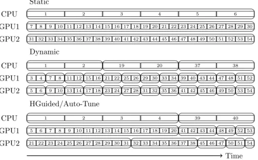
The behavior of the algorithms is illustrated in Figure 1. It shows the ideal
case in which in the execution of a regular application all devices finish
simul-taneously, thus achieving perfect load balance.
150
3.1. Static algorithm
This algorithm works before the kernel starts its execution by dividing the
dataset in as manypackagesas devices are in the system. The division relies on
knowing the computing power of the devices in advance. Then the execution
time of each device can be equalized by proportionally dividing the dataset
155
among the devices. As a consequence, there is no idle time in any device, which
would signify a waste of resources. The idea of assigning a single package to
each device is depicted in Figure 1.
A formal description of the algorithm can be made considering a
heteroge-neous system withndevices. Each deviceihascomputational power Pi, which
160
is defined as the amount of work that a device can complete per time unit,
including the communication overhead. This value depends on the architecture
of the device, but also on the application that is being run. These powers are
input parameters of the algorithm and can be extracted by a simple profiled
execution.
165
The application will execute a kernel overW work-items, grouped inG
work-groups of fixed sizeLs=WG. Since the work-groups do not communicate among
themselves, it makes sense to distribute the workload taking the work-group as the atomic unit. Each device i will have an execution time of Ti. Then the
execution time of the heterogeneous system will be that of the last device to
170
finish its work, orTH =maxni=1Ti. Also, since the whole system is capable of
executingW work-items inTH, it follows that its total computational power of
the heterogeneous system is PH = TW
H. Note that it also can be computed as
Static CPU 1 2 3 4 5 6 GPU1 7 8 9 10 11 12 13 14 15 16 17 18 19 20 21 22 23 24 25 26 27 28 29 30 GPU2 31 32 33 34 35 36 37 38 39 40 41 42 43 44 45 46 47 48 49 50 51 52 53 54 Dynamic CPU 1 2 19 20 37 38 GPU1 3 4 7 8 11 12 15 16 21 22 25 26 29 30 33 34 39 40 43 44 47 48 51 52 GPU2 5 6 9 10 13 14 17 18 23 24 27 28 31 32 35 36 41 42 45 46 49 50 53 54 HGuided/Auto-Tune CPU 1 2 3 4 39 40 GPU1 5 6 7 8 9 10 11 12 13 14 15 16 17 18 19 20 41 42 43 44 48 49 52 53 GPU2 21 22 23 24 25 26 27 28 29 30 31 32 33 34 35 36 37 38 45 46 47 50 51 54 Time
Figure 1: Depiction of how the four algorithms perform the data division among three devices. The work groups assigned to each device, identified by numbers, are joined in packages shown as larger rounded boxes. Note that the execution time of work groups in the CPU is four times larger than in the GPUs.
PH = W TH = n X i=1 Pi
The goal of the Static algorithm is to determine the number of work-groups
175
to assign each device, so that all the devices finish their work at the same time.
This means finding a tuple{α1, ...αn}, whereαi is the number of work-groups
assigned to the devicei, such that:
TH=T1=· · ·=Tn⇔ Lsα1
P1
=· · ·= Lsαn Pn
This set of equations can be generalised and solved as follows:
TH= Lsαi Pi ⇔αi = THPi Ls =THPiG W = PiG Pn i=1Pi
Sinceαiis the number of work-groups, its value must be an integer. For this
180
reason, the expression used by the algorithm is:
αi= P iG Pn i=1Pi
If there is not an exact solution with integers then Pn
i=1αi < G. In this
case, the remaining work-groups are assigned to the most powerful device.
The advantage of the Static algorithm is that it minimises the number of
synchronisation points. This makes it perform well when facing regular loads
185
with known computing powers that are stable throughout the dataset. However,
it is not adaptable, so its performance might not be as good with irregular loads.
3.2. Dynamic algorithm
Some applications do not present a constant load during their executions.
To adapt to their irregularities, the dynamic algorithm divides the dataset into
190
small packages of equal size. The number of packages is well above the number
of devices in the heterogeneous system. During the execution of the kernel,
a master thread in the host is in charge of assigning packages to the different
devices, following the next strategy:
1. The master splits theG work-groups in packages, each with the package
195
size specified by the user. This number must be a multiple of the
work-group size. If the number of work-items is not divisible by the package
size, the last package will be smaller
2. The master launches one package on each device, including the host itself
if it is desired.
200
3. The master waits for the completion of any package.
4. When deviceicompletes the execution of a package:
(a) The device returns the partial results corresponding to the processed
package.
(b) The master stores the partial results.
205
(d) If all the devices are idle and there are no more packages, the master
jumps to step 5.
(e) The master returns to step 3.
5. The master ends when all the packages have been processed and the results
210
have been received.
This behaviour is illustrated in Figure 1. The dataset is divided in small,
fixed size packages and the devices process them achieving equal execution time.
As a consequence, this algorithm adapts to the irregular behaviour of some
applications. However, each completed package represents a synchronisation
215
point between the device and the host, where data is exchanged and a new
package is launched. This overhead has a noticeable impact on performance. The Dynamic algorithm takes the size of the packages as a parameter.
3.3. HGuided algorithm
The two above algorithms are well known approaches to the problem of
220
load balancing in general. But none satisfy three key aspects. First, take into account the heterogeneity of the system. Second, control the overhead
of the synchronisation. And third, give reasonable performance with regular
or irregular applications. Thus a new load balancing algorithm method called
HGuided is proposed, which is based on theGuided method from OpenMP.
225
The main difference between the Hguided and the Dynamic Algorithm is the
size and quantity of the packets. In Dynamic, the size of the packets is constant,
while in HGuided they vary throughout the execution and between the devices.
As execution progresses, the size of the packets decreases with the remaining
workload. This size is weighted with the relative computational capacity of
230
each device. This way the less powerful devices (CPUs in this case) run smaller packets than they would in a homogeneous system, and the more powerful run
larger packets. The package size for devicei is calculated as follows:
package sizeH= $ Gr kN · Pi PN j=1Pj %
Note that the first term gives diminishing size of the packages, as a function
of the number of pending work-groups Gr, the number of devices N and the
235
constant k. The latter is introduced due to the unpredictable behavior of the irregular applications. It limits the maximum package size and, in the
exper-imental evaluation of Section 5, was empirically fixed to 2. The second term
adjusts the package size with the ratio of the computing capacity of the device
Pi to the total capacity of the system.
240
On the other hand, in the dynamic algorithm, the programmer sets the
number of packages for each execution. However, in the HGuided, since the size
of the packets depends on the device. Therefore, the number of packages will
vary according to the order in which the packets are assigned to the devices.
This can differ greatly between runs and especially in irregular applications.
245
Therefore, this algorithm reduces the number of synchronization points and the corresponding overhead, compared to the Dynamic.
Figure 1 shows how the size of the packages is large at the beginning of the
execution, and decreases towards the end.
3.4. Auto-Tune algorithm 250
The HGuided algorithm strikes a balance between adaptiveness and
over-heads, which makes it a good all-around solution that adequately distributes
the workload for both regular and irregular applications. However, it still
re-quires two parameters to be provided by the programmer: the computing power
and the minimum package size. These have a key impact on performance and are
255
dependent on both the application to be executed and the system itself.
More-over, the HGuided algorithm is quite sensitive to the parameters, so choosing
an adequate value for them is sometimes a demanding task that requires a
thor-ough experimental analysis. The sensitivity of the HGuided algorithm to its
parameters is further analyzed in Section 5.3.
260
In addition, determining the minimum package size parameter is
compli-cated, especially for GPUs, because it is essential to do a sweep to obtain a
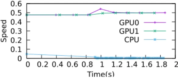
0 0.1 0.2 0.3 0.4 0.5 0.6 0 0.2 0.4 0.6 0.8 1 1.2 1.4 1.6 1.8 2 Speed Time(s) GPU0 GPU1 CPU
Figure 2: Speedup per application.
It only requires obtaining the response times in each device independently and
calculating the capacities.
265
The Auto-Tune algorithm is an evolution of the previous algorithm that
achieves near optimal performance for both regular and irregular loads without
the hassle of parameters. It uses the same formula to calculate the package size,
but uses nominal parameter values that are adjusted at runtime and handles
the minimum package size differently depending on the device that each package
270
will be sent to.
The computing power for the first package launched at each device is calcu-lated using the theoretical GFLOPs of the hardware. These can be obtained at
the installation of OmpSs either by querying the available devices or by running
a simple compute intensive benchmark. For the successive packages, the power
275
is updated taking into account the computing speed displayed by each device.
This is calculated as the average number of work-items processed per second for
the last three packages launched to each device. By using the average speed of
the last packages, a gradual adaptiveness is attained that keeps the algorithm
resistant to bursts of irregularity that would not be representative of the actual
280
speed for the next packages. Figure 2 depicts the evolution of the computing
power during the execution of one of the used for experimentation. The nominal computing powers are used at the beginning of the execution until all the devices
have finished at least one package. Then, the computing powers are updated
at runtime. In the figure, the nominal power for the GPU was higher than the
285
initial packages does not disturb the load balancing, as all the devices are kept
busy and do not delay the completion of the benchmark.
Package size also has an influence on the computing speed of throughput based architectures, such as GPUs. Consequently, package size must be kept
290
relatively high to prevent an inefficient use of the hardware and overheads.
However, this is also a potential source for imbalance. If the computing power of
the devices differs greatly, a high minimum package size that reduces overheads
is likely to be too big for slow devices, namely, CPUs, which would cause delays.
To prevent this, the Auto-Tune HGuided algorithm uses different minimum
295
values for CPUs and GPUs. The value selected for the CPU is one work-group
per CPU core, so no hardware is left unused and imbalance is avoided. This is
because the CPU is not a throughput device, so its computing speed is usually
much less sensitive to package size than the GPUs. Moreover, CPUs are often the least powerful device of the system, so using a small minimum package size
300
with them will improve the load balancing. Two values are considered for the
GPU minimum package size. First, the equations implemented in the CUDA
Occupancy Calculator are used to obtain the minimum number of work-groups
that will achieve maximum occupancy for the current kernel and GPU. The
CUDA Occupancy Calculator is part of the CUDA Toolkit since version 4.1.
305
This value is a lower bound for the minimum package size, but might be too low
if the application launches a large amount of work-items, producing too many
packages and high overheads. To prevent this, the number of work-items is also
analyzed and the final minimum package size is set to the maximum between the value obtained the Occupancy Calculator and 5% of the work-items. This
310
percentage has been experimentally set to keep the number of packages low and
avoid performance degradation in the GPU.
These enhancements give forth an algorithm with improved adaptiveness,
that delivers comparable performance to the HGuided approach for a fraction
of the effort. It completely eliminates the need to provide any parameter and
315
saves a great deal of pre-processing time per application and system, as will be
4. Implementation
As stated before, the OmpSs infrastructure relies on the combination of two
components: Mercurium, which is a source-to-source compiler, and Nanos++,
320
which is a runtime capable of managing tasks, their data and the Task
De-pendence Graph (TDG)they generate. As a first approach, the new load
bal-ancing algorithms have been implemented focusing on making the changes as
self-contained as possible and minimizing the impacts on the OmpSs
specifica-tion, Mercurium and the rest of Nanos++. As a result, neither directives nor
325
clauses have been added to Mercurium. Nanos++ implements a set of
differ-ent schedulers that deal with the managemdiffer-ent of the tasks submitted to the
runtime. To offer the work distribution strategies for a single OpenCL task
presented in the previous section, a new scheduler has been implemented as a
Nanos++ plugin, which has been calledmaat. The parameters of the algorithms
330
are the following:
• The device computing powers for Static and HGuided. • The package size for Dynamic.
• The minimum package size for HGuided.
To avoid altering the OmpSs specification, the selected algorithm and its
pa-335
rameters are set through environment variables, which is the normal way to
specify the scheduler in Nanos++.
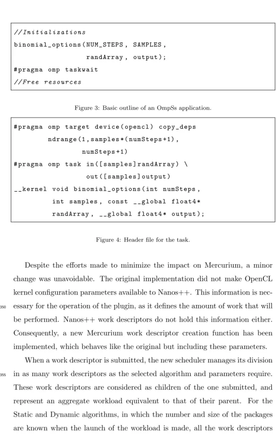
Figure 3 represents the outline of an OmpSs implementation of the Binomial benchmark used later in the experimentation. It shows how a call to a function
defined as a task is followed by a wait. The header of that function, which is
340
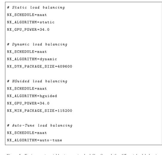
shown in Figure 4, indicates that the task must be run in an OpenCL device,
as well as its launch parameters, input and output data. Figure 5 displays the
environment variables that need to be set to run the task with each of the four
algorithms presented in Section 3. As shown, the selection of the auto-tune
algorithm eliminates the need of specifying any other load balancing related
345
// I n i t i a l i z a t i o n s
b i n o m i a l _ o p t i o n s ( N U M _ S T E P S , SAMPLES , r a n d A r r a y , o u t p u t ); # p r a g m a omp t a s k w a i t
// F r e e r e s o u r c e s
Figure 3: Basic outline of an OmpSs application.
# p r a g m a omp t a r g e t d e v i c e ( o p e n c l ) c o p y _ d e p s n d r a n g e (1 , s a m p l e s *( n u m S t e p s +1) , n u m S t e p s +1) # p r a g m a omp t a s k in ([ s a m p l e s ] r a n d A r r a y ) \ out ([ s a m p l e s ] o u t p u t ) _ _ k e r n e l v o i d b i n o m i a l _ o p t i o n s ( int n u m S t e p s , int samples , c o n s t _ _ g l o b a l f l o a t 4 * r a n d A r r a y , _ _ g l o b a l f l o a t 4 * o u t p u t );
Figure 4: Header file for the task.
Despite the efforts made to minimize the impact on Mercurium, a minor
change was unavoidable. The original implementation did not make OpenCL kernel configuration parameters available to Nanos++. This information is
nec-essary for the operation of the plugin, as it defines the amount of work that will
350
be performed. Nanos++ work descriptors do not hold this information either.
Consequently, a new Mercurium work descriptor creation function has been
implemented, which behaves like the original but including these parameters.
When a work descriptor is submitted, the new scheduler manages its division
in as many work descriptors as the selected algorithm and parameters require.
355
These work descriptors are considered as children of the one submitted, and
represent an aggregate workload equivalent to that of their parent. For the
Static and Dynamic algorithms, in which the number and size of the packages are known when the launch of the workload is made, all the work descriptors
# S t a t i c l o a d b a l a n c i n g N X _ S C H E D U L E = m a a t N X _ A L G O R I T H M = s t a t i c N X _ G P U _ P O W E R = 3 4 . 0 # D y n a m i c l o a d b a l a n c i n g N X _ S C H E D U L E = m a a t N X _ A L G O R I T H M = d y n a m i c N X _ D Y N _ P A C K A G E _ S I Z E = 4 0 9 6 0 0 # H G u i d e d l o a d b a l a n c i n g N X _ S C H E D U L E = m a a t N X _ A L G O R I T H M = h g u i d e d N X _ G P U _ P O W E R = 3 4 . 0 N X _ M I N _ P A C K A G E _ S I Z E = 1 1 5 2 0 0 # Auto - T u n e l o a d b a l a n c i n g N X _ S C H E D U L E = m a a t N X _ A L G O R I T H M = auto - t u n e
Figure 5: Environment variables to use standard OmpSs and the different load balancing algorithms.
are created at the submission of their parent. They are stored in the scheduler
360
and adequately returned when a thread is idle, receptive to another task. In
the case of the HGuided and Auto-Tune algorithms, the packages have varying sizes that depend on the prior execution and the device that will run them. As
a consequence, the children work descriptors will be created when required by
an idle thread, considering the device it manages and the execution.
365
Each of the children work descriptors is identical to its parent except for two
key differences. First, it has different OpenCL parameters, namelyoffset and
output data is just a portion of that of its parent, which is conveniently offset
so the results are written adequately. This is represented by an independent
370
CopyDataobject, holding the start address and size that the package will have
to work on. As a result, coherence problems are avoided in the OmpSs directory.
Apart from the aforementioned details, data transfer relies on the methods used
by standard OmpSs. To perform the correspondence between work descriptors
and output data, an assumption is made: each OpenCL work-item will produce
375
the result for the position of the output buffers indexed by its identifier. This
may seem a strong requirement, but it is met by most kernels widely used in
the industry and research.
The creation of the children work descriptors is performed by a modified
version of theduplicateWD function that does this extra work. This function
380
is also responsible for making the OpenCL parameters of the divided work descriptors available to the Mercurium code, which will trigger the actual kernel
launches.
Once the submission of the original work descriptor is completed, the done
function is called. This is a Nanos++ function that is used to signal the
com-385
pletion of a work descriptor. It also waits for the completion of the children
of the calling work descriptor. In this way, no task dependent on the divided
one will be run until all the children resulting from the work distribution are
completed, so the dependencies of the task graph are maintained.
5. Evaluation
390
This Section begins with a description of the system and the benchmarks
used in the experiments, as well as definitions of the metrics used in the
evalu-ation. Additionally experimental results are showed and analyzed.
5.1. System Set-up
The test machine has two processor chips and two GPUs and 16 GBs of
395
run two threads each at 2.0 GHz. They are connected via QPI, which allows
OpenCL to detect them as a single device. Thus, any reference to the CPU
considers both processors. The GPUs are NVIDIA Kepler K20m with 13 SIMD lanes and 2496 cores and 5 GBytes of VRAM each. These are connected to the
400
system using independent PCI 2.0 slots.The experiments build upon a baseline
system which uses a single GPU but consider the static energy of all the devices,
regardless of if they are contributing work or not.
Six applications have been chosen for the experimentation. Three of them:
NBody,Krist andPerlin are part of the OmpSs examples offered by BSC, and
405
the other three: Binomial,Sparse Matrix and Vector product (SpMV) andRap
have been specifically adapted to OmpSs from existing OpenCL applications.
The first four (NBody, Krist, Binomial and Perlin) are regular, meaning that all
the work-groups represent a similar amount of work. On the contrary, SpMV and Rap are irregular, which implies that each work-group represents a
differ-410
ent amount of work. The parameters associated to each of the load balancing
algorithms have been set to maximize performance.The computing power for
a device/application pair has been obtained as the relative performance of the
device, with respect to that of the fastest device for the application.
Perlin implements an algorithm that generates noise pixels to improve the
415
realism of moving graphics. Krist is used on crystallography to find the exact
shape of a molecule using R¨ontgen diffraction on single crystals or powders.
Rap is an implementation of the Resource Allocation Problem. It has a certain
pattern in its irregularity, because each successive package represents an amount of work larger than the previous.
420
The evaluation of the performance of the benchmarks is done through their
response time. This includes the time required by the communication between
host and the devices, comprising input data and result transfer, as well as
the execution time of the kernel itself. The benchmarks are executed in two
scenarios, theheterogeneous system, taking advantage of the GPUs and CPU,
425
and the baseline, that only uses one GPU. Note that in both instances, the
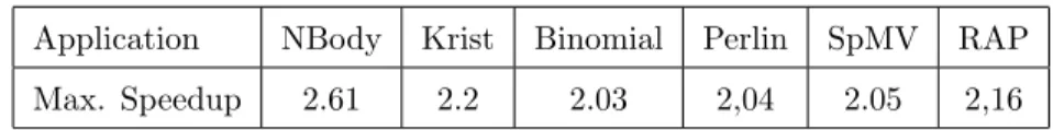
Table 1: Maximum achievable speedup per application.
Application NBody Krist Binomial Perlin SpMV RAP
Max. Speedup 2.61 2.2 2.03 2,04 2.05 2,16
recompile, only set environment variables.
Based on these response times, two metrics are analyzed. The first is the
speedup for each benchmark when comparing the baseline and the heterogeneous
430
system response times. Note that, for the employed benchmarks, the CPU is
much less powerful than the GPUs, then the maximum achievable speedup using
the three devices is not 3, but a fraction over 2 which depends on the computing
power of the CPU for the application. The speedup for each application using
a perfectly balanced work distribution is shown in Table 1. These values give
435
an idea of the advantage of using the complete system. They were derived from
the response timeTi of each device as shown in Equation 1.
Smax= 1 maxn i=1{Ti} n X i=1 Ti (1)
The second metric is the load balancing efficiency, obtained by dividing the
reached speedup by the maximum speedup, shown in Table 1. The obtained
value ranges between 0 and 1 giving an idea of the usage of the heterogeneous
440
system. Efficiencies close to 1 indicate the best usage of the system is being
made. The measured values do not reach this ideal because of the
communica-tion and synchronizacommunica-tion times between the host and the devices.
5.2. Energy measurement
To evaluate the energy efficiency of the system it is necessary to take into
445
account the power drawn by each device. Modern computing devices include
Performance Management Units (PMU)that allow applications to measure and
control the power consumption. However, the power measured is associated to
it is impractical to add measurement code to all the test applications, this led to
450
the development of a power monitoring tool namedSauna. It takes a program
as its parameter, and is able to configure the PMUs of the different devices in the system, run the program while performing periodic power measurements.
This tool required an unexpected amount of thought for its development.
Since it had to monitor several PMUs, it had to adapt to the particularities of
455
each one while giving consistent and homogeneous output data. For instance,
each device has a different way to access its PMUs. Recent versions of the Linux
kernel provides access to theRunning Average Power Limit (RAPL) registers
[13] of the Intel processors, which provide accumulative energy readings. On
contrast, NVIDIA provides a library to access their PMUs. But thisNVIDIA 460
Management Library (NVML)[14] gives instant power measurements.
During the development of Sauna, it was observed that these energy or power readings have an impact on the kernel or process execution. Then, finding an
adequate sampling period is an important task. To strike a balance between
the overhead that was observed in the GPUs with high sampling rates and
465
the accuracy loss that is inherent of lower ones, it was decided to use 45ms
as the sampling period. The performance and the energy consumption can be
combined in a single metric representing the energy efficiency of the system.
This paper uses the Energy Delay Product (EDP) [15] for this purpose.
5.3. Parameter sensitivity 470
As explained in Section 3, the Static, Dynamic and HGuided algorithms
require different parameters for their operation. These have to be provided by
the programmer and are one of the key factors for a successful load balancing.
However, determining the most adequate values for a workload is not trivial, as
they may differ greatly between applications and device configurations.
Conse-475
quently, the selection of parameters is often a work intensive process, usually based on experimentation.
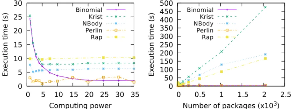
The importance of adequately choosing the parameter values is illustrated in
0 5 10 15 20 25 30 0 5 10 15 20 25 30 35 Ex ecution time (s) Computing power Binomial Krist NBody Perlin Rap
(a) Execution time with different computing powers for the Static algorithm.
0 50 100 150 200 250 300 350 400 450 500 0 0.5 1 1.5 2 2.5 Ex ecution time (s) Number of packages (x103) Binomial Krist NBody Perlin Rap
(b) Execution time with different numbers of packages for the Dynamic algorithm.
0 5 10 15 20 0 5 10 15 20 25 30 35 Ex ecution time (s) Computing power Binomial Krist NBody Perlin Rap
(c) Execution time with different computing powers for the HGuided algorithm.
0 10 20 30 40 50 60 70 0 0.2 0.4 0.6 0.8 1 1.2 1.4 Ex ecution time (s)
Minimum package size (x106) Binomial
Krist NBody Perlin Rap
(d) Execution time with different minimum package sizes for the HGuided algorithm. Figure 6: Parameter sensitivity analysis
the parameters for each of the algorithms. Note that for the HGuided
algo-480
rithm, when one of the parameters is modified, the other is set to the identified
optimal value. As shown in the figure, for every of the parameters, the applica-tions show very different behaviors, ranging from near insensitivity to delivering
greatly degraded performance, sometimes even lacking a clear relation with the
parameter value, as is for example the case of Rap for the minimum package
485
size. Moreover, the applications are not affected equally by the parameters. For
example, Binomial is highly sensitive to the computing power in the Static
algo-rithm and moderately sensitive to almost insensitive to the rest of parameters,
while Rap behaves just the opposite: it is insensitive to the Static computing
power and tremendously sensitive to the other parameters.
490
Considering these results, it is obvious that, in order to achieve an accurate
load balancing, an experimental tuning of the algorithm parameters is often a must. The Auto-Tune algorithm frees the programmer from this burden by
automatically adjusting the parameters, matching and even surpassing the
per-formance of the HGuided.
495
5.4. Experimental results
The experiments presented in this section have been developed with the
optimal values for the parameters required by each algorithm, obtained in the
previous section. This implies that the results for the static, dynamic and
HGuided algorithms are the best that can be achieved, but require a great
500
effort to tune the parameters.
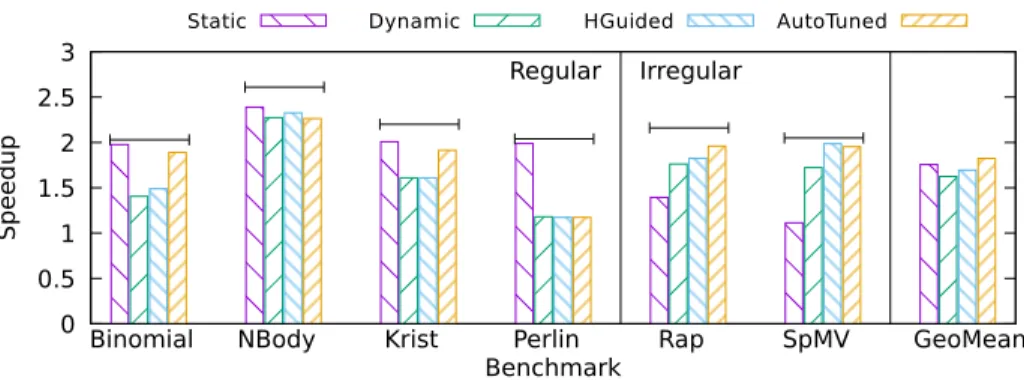
Figure 7 shows the speedup obtained for each application calculated with
respect to their execution time using the baseline system, as was explained in
Section 5.1. This section also showed that the maximum achievable speedup
depends on the application. These values, presented in Table 1, are shown in
505
the graph as horizontal lines above each benchmark. Additionally, the geometric mean is shown, which includes both four regular benchmarks and two irregular
ones.
0 0.5 1 1.5 2 2.5 3
Binomial NBody Krist Perlin Rap SpMV GeoMean
Regular Irregular
Speedup
Benchmark
Static Dynamic HGuided AutoTuned
Figure 7: Speedup per application.
is obtained by the Auto-Tune algorithm, closely followed by the Static, the
510
HGuided and finally the Dynamic. Furthermore, it should be emphasized that
the Auto-Tune algorithm is much easier to use, because it does not require
finding optimal values for any parameter.
A detailed analysis of the speedups reveals that the Static algorithm is the
best option for regular applications. However, except in the case of Perlin, the
515
Auto-Tune algorithm achieves very similar results, with less effort. The other
two algorithms achieve good results, however suffer from a problem that reduces
performance. If one of the last packages is assigned to the slowest device it is likely to delay the execution of the whole application. This problem could be
avoided by increasing the number of packages, but in that case overheads come
520
into play, which also degrades performance. The HGuided algorithm due to its
very nature, partially solves this issue.
For irregular applications, the best results are obtained by Auto-Tune and
HGuided algorithms. Their adaptive behaviour favours load balancing in these
applications, where the workload of each work-group is completely unknown
525
and unpredictable. On the other hand, the reduction in synchronization points
reduces the runtime overhead, which is inherent to this type of algorithm.
Fi-nally, the Static algorithm fails to balance the load because it can not cope with the irregularity of these applications.
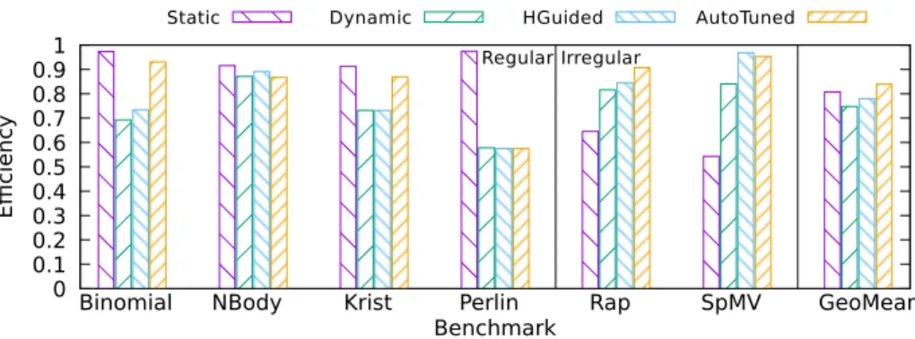
The load balancing efficiency gives an idea of how well a load is balanced. A
0 0.1 0.2 0.3 0.4 0.5 0.6 0.7 0.8 0.9 1
Binomial NBody Krist Perlin Rap SpMV GeoMean
Regular Irregular
E
ffi
ciency
Benchmark
Static Dynamic HGuided AutoTuned
Figure 8: Efficiency of the heterogeneous system.
value of one represents that all the devices have been working all the time, thus
achieving the maximum speedup. In Figure 8 the geometric mean efficiencies
show that the best result is achieved by Auto-Tune with a efficiency around
0.85. In addition, there is at least one load balancing algorithm for every
ap-plication that achieves an efficiency over 0.9. This is true even for the irregular
535
applications, in which obtaining a balanced work distribution is significantly
harder. In general it can be said that the efficiency can be largely improved,
for instance it can be as high as 0.98, reached by Binomial and Perlin with the
Static.
Nowadays, performance is not the only figure of merit used to evaluate
com-540
puting systems. Their energy consumption and efficiency are also very
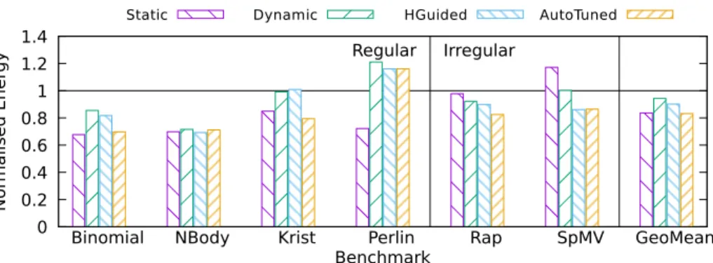
impor-tant. Figure 9 gives an idea of the energy saving the whole heterogeneous system
brings, compared to the baseline system. The latter only uses one GPU while
the other devices are idle and still consuming. Therefore, the Figure shows for
each benchmark the energy consumption of each algorithm normalized to the
545
baseline consumption, meaning that less is better.
The values of the geometric mean indicate that the algorithms that consume
less energy are Static and Auto-Tune, with a saving of almost 20% compared
to the baseline. Moreover, all the algorithms reduce consumption, despite using the whole system. Regarding the individual benchmarks, it is always possible
550
0 0.2 0.4 0.6 0.8 1 1.2 1.4
Binomial NBody Krist Perlin Rap SpMV GeoMean Regular Irregular
Nor
malised Ener
gy
Benchmark
Static Dynamic HGuided AutoTuned
Figure 9: Normalised energy consumption per application.
more devices necessarily increases the instantaneous power at any time. But,
since the total execution time is reduced, the total energy consumption is also
less. This saving is further improved by the fact that idle devices still consume
energy, so making all devices contribute work is beneficial.
555
The analysis of the algorithms shows a strong correlation between
perfor-mance and energy saving. Consequently, the best algorithm for regular
applica-tions is also the Static, with an average saving of 26.5%. However, for irregular
applications, it wastes 7.4% of energy. On the other hand, the Auto-Tune gives
an average energy saving of 16% regardless of the kind of application.
560
Regarding the results of concrete benchmarks, it is interesting to comment
Krist. In this benchmark the highest energy saving is provided by Auto-Tune,
although it is not the best in performance. There are only two particular cases
where the use of the whole system employs more energy than the baseline. These
are Perlin with Dynamic, Hguided and Auto-Tune, and SpMV with Static. This
565
is because, in all other algorithms, the gain in performance is too small and
cannot compensate for the increased power consumption involved in using the
complete system.
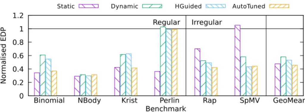
Another interesting metric is the energy efficiency, which combines
perfor-mance with consumption. With the dual goal of low energy and fast execution
570
in mind, theEnergy Delay Product (EDP) is the product of the consumed
0 0.2 0.4 0.6 0.8 1 1.2
Binomial NBody Krist Perlin Rap SpMV GeoMean
Regular Irregular
Nor
malised EDP
Benchmark
Static Dynamic HGuided AutoTuned
Figure 10: Normalised EDP per application.
algorithms normalised to the EDP of the baseline.
Since the EDP is a combination of the two above metrics, the previous
results are further corroborated it. Therefore Auto-Tune also achieves the best
575
energy efficiency results on geometric mean, followed by Static, Hguided and
Dynamic. Attending to the individual algorithms, their relative advantages is also maintained. Although the Static algorithm on regular applications shows a
significant reduction of the EDP of 65%, the same is not true on irregular ones,
reducing only 12.4%. In contrast, the Auto-Tune is more reliable, as it achieves
580
a similar reduction on both kinds of applications; 48% on regular and 57% on
irregular.
6. Related Work
Heterogeneity has taken computing platforms by storm, ranging from HPC systems to hand-held devices. The reason for this is their outstanding
per-585
formance and energy efficiency. However, making the most of heterogeneous
systems also poses new challenges. The extra computing power also involves
new decisions on how to use all the available hardware, which currently have
to be made by the programmer without much help from the programing
frame-works and runtimes. The keys to make programming easy again are system
590
abstraction, so the heterogeneous devices are handled transparently, and load
are, these problems are often addressed separately.
To the load balancing problem alone, there are two main approaches found
in the literature: static anddynamic, which in turn can be adaptive or not.
595
Regarding static methods, Leeet al.[16] propose the automatic modification
of OpenCL code that executes on a single device, so the load is balanced among
several. De la Lamaet al. [17] propose a library that implements static load
balancing by encapsulating standard OpenCL calls. The work presented in
[18] uses machine learning techniques to come up with an offline model that
600
predicts an ideal static load partitioning. However, this model does not consider
irregularity. Similarly, Zhonget al. [19] use performance models to identify an
ideal static work distribution. In [20] the focus is on the static distribution of
a single kernel execution to the available devices via code modifications. Qilin
[21] is a training-based work distribution method that propose to balance the
605
load using a database containing execution-time data for all the programs the
system has executed and a linear regression model. This technique is only useful
in systems that run the same applications frequently.
In the dynamic approach [22, 23] propose different techniques and runtimes.
However, these focus on task distribution and not on the co-execution of a single
610
data parallel kernel. The work of [24] deals with the dynamic distribution of
TBB parallel for loops, adapting block size at each step to improve balancing.
FluidicCL [5] does focus on co-execution but for systems with a CPU and a
GPU. SnuCL [4] also tackles data parallelism, but is mostly centered on the
distribution of the load among different nodes using an OpenCL-like library.
615
Kaleem’s et al. proposal in [7] and Boyer’s et al. in [6] propose adaptive
methods that use the execution time of the first packages to distribute the
re-maining load. However, they focus on a CPU/GPU scenario and do not scale
well to configurations with more devices. Similarly, HDSS [25] is a load
balanc-ing algorithm that dynamically learns the computational power of each
proces-620
sor during an adaptive phase and then schedules the remainder of the workload
using a weighted self-scheduling scheme during the completion phase.
representative of the whole load, which might not be true for irregular kernels.
Besides, package size decreases linearly during the completion phase, which may
625
produce unnecessary overheads as substantiated in this paper. Navarro et al.
[24] propose a dynamic, adaptive algorithm for TBB that uses a fixed package
size for the GPU and a variable one for the CPU to try to achieve good
bal-ancing. This work was extended in [26], proposing an adaptive package size for
the GPU too. This is also based on using small initial packages to identify a
630
package size that obtains near optimal performance.
Scoglandet al. [27] propose several work distribution schemes that fit
differ-ent accelerated OpenMP computing patterns. However, they do not propose a
single solution to the load balancing problem. The library presented in [28] also
implements several load balancing algorithms and proposes the HGuided, which
635
adapts to irregularity and considers heterogeneity. This library is also used in Xeon Phi base systems in [29]. However, it requires certain parameters from
the programmer that may not be easy to obtain and uses linearly decreasing
packages that might incur overheads.
Some papers propose algorithms to distribute the workload between CPU
640
and GPU taking performance and power into account. For instance, GreenGPU
dynamically distributes work to GPU and CPU, minimizing the energy wasted
on idling and waiting for the slower device [30]. To maximize energy savings
while allowing marginal performance degradation, it dynamically throttles the
frequencies of CPU, GPU and memory, based on their utilizations. Wang and
645
Ren [31] propose a power-efficient load distribution method for single applica-tions on CPU-GPU systems. The method coordinates inter-processor work
dis-tribution and frequency scaling to minimize energy consumption under a length
constraint. SPARTA is a throughput-aware runtime task allocator for
Hetero-geneous Many Core platforms [32]. It analyzes tasks at runtime and uses the
650
obtained information to schedule the next tasks maximizing energy-efficiency.
With respect to the problem of transparently managing a heterogeneous
system, the authors of [33] propose a framework for OpenCL that enables the
present an interesting architecture-supported take on efficient, transparent data
655
distribution among several GPUs. Nevertheless, this works overlook load
bal-ancing, which is essential when trying to make the most of several heterogeneous devices. Maestro [34] implements concepts related to the abstraction of the
sys-tem, but the load balancing algorithm it proposes requires training.
You [35], Zhong [8] and Ashwin [36] do address both load balancing while
660
abstracting the underlying system and data movement. Nevertheless, their focus
is on task-parallelism instead of on the co-execution of a single data-parallel
kernel. Kim et al. [37] approach the problem by implementing an OpenCL
framework that provides the programmer with a view of a single device by
transparently managing the memory of the devices. Their approach is based on
665
a Static load balancing strategy, so it can not adapt to irregularity. Besides,
they only consider systems with several identical GPUs, lacking the adaptability that OmpSs offers.
There are also some contributions that focus on scheduling and load
balanc-ing for OmpSs tasks. For instance, the scheduler presented in [38] is closer to
670
the idea of co-execution. It holds several implementations of a task, targeted for
different devices, that will be run iteratively. The scheduler stores the execution
time of each implementation, so it can take load balancing decisions on what
implementation is best to run next. However, the programmer is responsible for
mapping the computation on several iterative tasks, which may not be an easy
675
and natural approach for the application at hand.
7. Conclusions and Future Work
This paper presents a new scheduler of the OmpSs programming model that
allows to efficiently co-execute a single OpenCL kernel instance using all the
devices in a heterogeneous system. The scheduler has been conceived so that it
680
is fully transparent to the programmer, who only needs to select the algorithm and set its parameters through environment variables.
algo-rithms. These include the classic Static and Dynamic algorithms, as well as
a version of the Guided, called HGuided, that takes into account the
hetero-685
geneity of the system. Achieving good result with these algorithms required the tuning of several parameters. Therefore, this paper also presents a novel load
balancing algorithm called Auto-Tune, which is capable of determining suitable
parameter values for each application automatically.
Judging by the results of all the experiments presented in this paper, two
690
conclusions can be reached. First, the utilization of all the devices of a
het-erogeneous system to execute the benchmarks significantly improves their
per-formance, energy consumption and efficiency. Second, although there are some
particular cases in which the Static algorithm outperforms the Auto-Tune
algo-rithm, it achieves excellent results without a tedious and time-consuming phase
695
of parameter optimization, which would necessary for each new benchmark or system.
According to our experimental results, Auto-Tune is capable of taking
ad-vantage of the whole heterogeneous system, with an average efficiency of 0.85.
Since the all the compute devices of the machine are used, the execution time is
700
reduced and consequently, an average energy saving of 16% has been observed.
The combination of these two improvements gives an reduction of the EDP close
to 50%.
The future of this extension will see compatibility with new devices, like
Intel Xeon Phi, FPGAs or integrated GPUs. From the OmpSs perspective, a
705
modification of the pragma specification would allow the programmer to select different algorithms or parameters for different kernels of the same application.
It would be interesting to extend the evaluation to different systems and device
configurations.
Acknowledgments
710
This work has been supported by the University of Cantabria with grant
Spanish Ministry of Economy, Industry and Competitiveness under contracts
TIN2016-76635-C2-2-R (AEI/FEDER, UE) and TIN2015-65316-P. The
Span-ish Government through the Programa Severo Ochoa (SEV-2015-0493). The
715
European Research Council under grant agreement No 321253 European
Com-munity’s Seventh Framework Programme [FP7/2007-2013] and Horizon 2020
under the Mont-Blanc Projects, grant agreement No 288777, 610402 and 671697
and the European HiPEAC Network.
References
720
[1] J. Nickolls, I. Buck, M. Garland, K. Skadron, Scalable parallel programming
with cuda, Queue 6 (2) (2008) 40–53.
[2] J. E. Stone, D. Gohara, G. Shi, OpenCL: A parallel programming standard
for heterogeneous computing systems, IEEE Des. Test 12 (3) (2010) 66–73.
[3] J. Cabezas, I. Gelado, J. E. Stone, N. Navarro, D. B. Kirk, W. m. Hwu,
725
Runtime and architecture support for efficient data exchange in
multi-accelerator applications, IEEE Transactions on Parallel and Distributed
Systems 26 (5) (2015) 1405–1418.
[4] J. Kim, S. Seo, J. Lee, J. Nah, G. Jo, J. Lee, SnuCL: An opencl framework
for heterogeneous CPU/GPU clusters, in: Proceedings of the ACM ICS,
730
ACM, New York, NY, USA, 2012, pp. 341–352.
[5] P. Pandit, R. Govindarajan, Fluidic kernels: Cooperative execution of
opencl programs on multiple heterogeneous devices, in: Proceedings of
Annual IEEE/ACM CGO, ACM, 2014, p. 273:283.
[6] M. Boyer, K. Skadron, S. Che, N. Jayasena, Load Balancing in a Changing
735
World: Dealing with Heterogeneity and Performance Variability, in: Proc. of the ACM Int. Conference on Computing Frontiers, ACM, New York,
[7] R. Kaleem, R. Barik, T. Shpeisman, B. T. Lewis, C. Hu, K. Pingali,
Adap-tive heterogeneous scheduling for integrated GPUs, in: Proc. of PACT,
740
ACM, New York, NY, USA, 2014, pp. 151–162.
[8] J. Zhong, B. He, Kernelet: High-throughput GPU kernel executions with
dynamic slicing and scheduling, CoRR abs/1303.5164.
[9] A. Duran, E. Ayguad´e, R. M. Badia, J. Labarta, L. Martinell, X. Martorell,
J. Planas, Ompss: A proposal for programming heterogeneous multi-core
745
architectures, Parallel Processing Letters 21 (02) (2011) 173–193.
[10] F. Sainz, S. Mateo, V. Beltran, J. L. Bosque, X. Martorell, E. Ayguad´,
Leveraging ompss to exploit hardware accelerators, in: Int. Symp. on
Com-puter Architecture and High Performance Computing, 2014, pp. 112–119.
[11] Mercurium C/C++/Fortran source-to-source compiler, last accesed April
750
2018.
URLhttps://github.com/bsc-pm/mcxx
[12] Nanos++ Runtime Library, last accesed April 2018.
URLhttps://github.com/bsc-pm/nanox
[13] E. Rotem, A. Naveh, D. Rajwan, A. Ananthakrishnan, E. Weissmann,
755
Power management architecture of the 2nd generation Intel Core
microar-chitecture, formerly codenamed Sandy Bridge, in: IEEE Int. HotChips
Symp. on High-Perf. Chips, 2011.
[14] NVIDIA, Management Library (NVML), last accesed November 2016. URLhttps://developer.nvidia.com/nvidia-management-library-nvml
760
[15] E. Castillo, C. Camarero, A. Borrego, J. L. Bosque, Financial applications
on multi-cpu and multi-gpu architectures, J. Supercomput. 71 (2) (2015)
729–739.
[16] J. Lee, M. Samadi, Y. Park, S. Mahlke, Transparent CPU-GPU
Collab-oration for Data-parallel Kernels on Heterogeneous Systems, in: Proc. of
765
[17] C. S. de la Lama, P. Toharia, J. L. Bosque, O. D. Robles, Static multi-device
load balancing for opencl, in: Proc. of ISPA, IEEE Computer Society, 2012,
pp. 675–682.
[18] K. Kofler, I. Grasso, B. Cosenza, T. Fahringer, An automatic
input-770
sensitive approach for heterogeneous task partitioning, in: Proceedings of
the 27th International ACM Conference on International Conference on
Supercomputing, ICS ’13, ACM, New York, NY, USA, 2013, pp. 149–160.
doi:10.1145/2464996.2465007.
URLhttp://doi.acm.org/10.1145/2464996.2465007
775
[19] Z. Zhong, V. Rychkov, A. Lastovetsky, Data partitioning on multicore
and multi-gpu platforms using functional performance models,
Comput-ers, IEEE Trans. on 64 (9) (2015) 2506–2518.
[20] J. Lee, M. Samadi, Y. Park, S. Mahlke, Skmd: Single kernel on multiple
devices for transparent cpu-gpu collaboration, ACM Trans. Comput. Syst.
780
33 (3) (2015) 9:1–9:27.
[21] C.-K. Luk, S. Hong, H. Kim, Qilin: Exploiting parallelism on
heteroge-neous multiprocessors with adaptive mapping, in: Proc. of the 42Nd
An-nual IEEE/ACM International Symposium on Microarchitecture, MICRO
42, ACM, New York, NY, USA, 2009, pp. 45–55.
785
[22] T. Gautier, J. Lima, N. Maillard, B. Raffin, Xkaapi: A runtime system for
data-flow task programming on heterogeneous architectures, in: IPDPS, 2013, pp. 1299–1308.
[23] A. Haidar, C. Cao, A. Yarkhan, P. Luszczek, S. Tomov, K. Kabir, J.
Don-garra, Unified development for mixed multi-GPU and multi-coprocessor
en-790
vironments using a lightweight runtime environment, in: Proc. of IPDPS,
2014, pp. 491–500.
utilization on multi-CPU and multi-GPU heterogeneous architectures, J.
Supercomput. 70 (2) (2014) 756–771.
795
[25] M. E. Belviranli, L. N. Bhuyan, R. Gupta, A dynamic self-scheduling scheme for heterogeneous multiprocessor architectures, ACM Trans. Archit.
Code Optim. 9 (4) (2013) 57:1–57:20. doi:10.1145/2400682.2400716.
URLhttp://doi.acm.org/10.1145/2400682.2400716
[26] A. Vilches, R. Asenjo, A. Navarro, F. Corbera, R. Gran, M. Garzarn,
800
Adaptive partitioning for irregular applications on heterogeneous
cpu-gpu chips, Procedia Computer Science 51 (2015) 140 – 149,
international Conference On Computational Science, ICCS 2015.
doi:https://doi.org/10.1016/j.procs.2015.05.213.
URL http://www.sciencedirect.com/science/article/pii/
805
S1877050915010212
[27] T. Scogland, B. Rountree, W. chun Feng, B. de Supinski, Heterogeneous
task scheduling for accelerated openmp, in: Proc. IPDPS, 2012, pp. 144–
155.
[28] B. P´erez, J. L. Bosque, R. Beivide, Simplifying programming and load
810
balancing of data parallel applications on heterogeneous systems, in:
Pro-ceedings of the 9th Annual Workshop on General Purpose Processing Using
Graphics Processing Unit, GPGPU ’16, ACM, New York, NY, USA, 2016,
pp. 42–51. doi:10.1145/2884045.2884051.
URLhttp://doi.acm.org/10.1145/2884045.2884051
815
[29] R. Nozal, B. Perez, J. L. Bosque, R. Beivide, Load balancing in a
het-erogeneous world: Cpu-xeon phi co-execution of data-parallel kernels, The
Journal of Supercomputingdoi:10.1007/s11227-018-2318-5.
URLhttps://doi.org/10.1007/s11227-018-2318-5
[30] K. Ma, X. Li, W. Chen, C. Zhang, X. Wang, Greengpu: A holistic approach
820
to energy efficiency in gpu-cpu heterogeneous architectures, in: 2012 41st
[31] G. Wang, X. Ren, Power-efficient work distribution method for cpu-gpu
heterogeneous system, in: Int. Symp. on Parallel and Distributed
Process-ing with Applications, 2010, pp. 122–129.
825
[32] B. Donyanavard, T. M¨uck, S. Sarma, N. Dutt, Sparta: Runtime task
al-location for energy efficient heterogeneous many-cores, in: Int. Conf. on
Hardware/Software Codesign and System Synthesis, CODES ’16, ACM,
New York, NY, USA, 2016, pp. 27:1–27:10.
[33] A. L. R. Tupinamb´a, A. Sztajnberg, Transparent and optimized distributed
830
processing on gpus, IEEE Trans. on Parallel and Distributed Systems
27 (12) (2016) 3673–3686.
[34] K. Spafford, J. Meredith, J. Vetter, Maestro: Data orchestration and
tun-ing for opencl devices, in: Proceedtun-ings of the 16th International Euro-Par Conference on Parallel Processing: Part II, Euro-Par’10, Springer-Verlag,
835
Berlin, Heidelberg, 2010, pp. 275–286.
URLhttp://dl.acm.org/citation.cfm?id=1885276.1885305
[35] Y.-P. You, H.-J. Wu, Y.-N. Tsai, Y.-T. Chao, Virtcl: A framework for
OpenCL device abstraction and management, in: Principles and Practice
of Parallel Programming, PPoPP 2015, ACM, 2015.
840
[36] A. M. Aji, A. J. Pe˜na, P. Balaji, W.-c. Feng, Multicl: Enabling automatic
scheduling for task-parallel workloads in opencl, Parallel Comput. 58 (C)
(2016) 37–55.
[37] J. Kim, H. Kim, J. Lee, J. Lee, Achieving a single compute device image
in OpenCL for multiple GPUs, in: Proc. of the ACM PPoPP., ACM, 2011,
845
pp. 277–287.
[38] J. Planas, R. M. Badia, E. Ayguad´e, J. Labarta, Self-adaptive ompss tasks
in heterogeneous environments, in: 2013 IEEE 27th Int. Symp. on Parallel