A Hybrid Parallel Neighbor-Joining Algorithm for
Phylogenetic Tree Reconstruction on a Multicore
Cluster
Enzo Rucci, Franco Chichizola, Marcelo Naiouf, Armando De Giusti
Instituto de Investigación en Informática LIDI (III-LIDI), Facultad de Informática, Universidad Nacional de La Plata Calle 50 y 120, 1900 La Plata (Buenos Aires), Argentina
[email protected]; [email protected]; [email protected]; [email protected]
Abstract-Building phylogenetic trees is one of the significant applications within bioinformatics, mainly due to its involvement in multiple sequence alignment. Because of the high computational complexity required, the use of parallel processing during the building process is convenient. Taking into account that current cluster architectures are hybrid, in this paper we present a parallel algorithm to build phylogenetic trees based on the Neighbor-Joining method, which uses a hybrid communication model (combination of message passing and shared memory), and then analyze its performance. Finally, conclusions and possible future lines of work are presented.
Keywords- Parallel Programming; Hybrid Programming; Multicore Cluster; Phylogenetic Trees; Neighbor-Joining Method
I. INTRODUCTION
Up to some years ago, the idea of a direct application of computer methods in natural sciences was odd and not very convincing. However, it is now evident that any serious advance in our knowledge and understanding of, for instance, the complex mechanisms of the cells, would be impossible without the help of powerful algorithms and fast computers.
Studies carried out on molecular mechanisms of organisms suggest that all organisms in the planet have a common predecessor. Then, any set of species would be related, which is called Phylogeny. In general, this relation can be represented by means of a phylogenetic tree. The task of Phylogeny is to infer the previous tree based on observations of the existing organisms [1].
Phylogenetic trees play an important role for several relevant applications within bioinformatics, such as multiple sequence alignment [2]. In general, multiple sequence
alignment comprises of three stages and the second stage generates a guided tree using some phylogeny reconstruction method.
There are various methods to build phylogenetic trees, including those of maximum probability and those based on distance matrixes. Maximum probability methods produce accurate results, but unfortunately are usually of an exponential order, which makes their use unfeasible for building large trees. Distance matrix-based methods use matrixes to define the distance between any pair of sequences. Even though its results are less accurate than those obtained with maximum probability methods, they are
of polynomial order and thus facilitate processing large data sets [3].
The Neighbor-Joining method (NJ) is based on distance matrixes and is widely used by biotechnologists and molecular biologists due to its efficiency and temporal complexity order. In recent years, it has become very popular through its use in the ClustalW algorithm [4], one of
the most widely used tools for multiple sequence alignment. The NJ algorithm was originally developed by Saitou and Nei in 1987 [5]. One year later, Studier and Keppler [6] would
review the algorithm and incorporate an improvement that allows reducing the temporal complexity from O(n5) to
O(n3).
Nowadays, thanks to the advances in sequentiation technologies, increasingly larger data sets can be obtained. Building a tree with thousands of taxa using the NJ method could take hours or days if a sequential algorithm is used due to its temporal complexity order (O(n3)). This makes it
suitable for parallel processing.
In the past decade, processors have improved their performance in accordance with Moore’s Law [7] mainly due
to two technology factors. The first of these was the increase in the frequency that can be achieved by processor's clock, and the second one was based on the increasing number of transistors in a chip. The combination of both factors with improvements in compilers allowed increasing the number of executable instructions per time unit. However, this improvement process was limited by the associated increase in temperature and energy use. To sustain the increase in the number of executable instructions per time unit, hardware architects developed processors with multiple cores. This type of processors integrates two or more computational cores within a single chip. Even though these cores are simpler and slower, when combined they allow enhancing the global performance of the processor while making a mire efficient use of energy [8] [9] [10].
The term cluster is applied to sets of computers built with standard hardware components that act as if they were a single computer [11]. Nowadays they are fundamental for the
solution of problems from the science, engineering, and modern commerce fields [12]. Cluster technology has evolved
to support activities that go from supercomputing applications and mission-critical software, web servers and e-commerce, to high-performance databases, among other uses.
The addition of multicore processors to traditional cluster architectures has led these to a new stage, giving birth to a hybrid parallel architecture known as multicore cluster [13].
The difference between a multicore cluster and a traditional cluster is that the former has one or more multicore processors in each node, rather than a single monocore processor. The cores that are within the same node communicate through the different memory levels of the node. The cores that are in different nodes, communicate by exchanging messages through the interconnecting network.
Parallel programming paradigms differ in the way tasks communicate and synchronize. In shared memory architectures, such as multicores, the most widely used paradigm is that of shared memory. In it, tasks communicate and synchronize by reading and writing variables in a shared address space. OpenMP is the most widely used library to program shared memory [14]. Message passing is the most
commonly chosen paradigm for distributed architectures, such as traditional clusters. In it, each task has its own address space and task communication and synchronization is done by exchanging messages. MPI is the most widely used library to program under this paradigm [15]. Multicore
clusters are hybrid architectures that combine distributed memory with shared memory. When it comes to programming parallel applications to be run on this type of architectures, a mixed paradigm that combines those described above is used. It is also possible to use message passing only, which involves simulating distributed memory over shared memory. However, this strategy is normally disregarded due to the loss in performance caused by the additional copies between the communication buffers from processes in the same node.
In this paper, a parallel algorithm is presented for building phylogenetic trees using the Neighbor-Joining method. This algorithm uses a hybrid communication model that combined message passing with shared memory, and is appropriate for execution on hybrid architectures such as multicore clusters. The remaining sections of this paper are organized as follows: in Section II, other works that are related to this research are presented. In Section III, the Neighbor-Joining method is described in detail. The algorithms developed are discussed in Section IV. Then, in Section V and Section VI, the experimental work carried out and the results obtained are described, respectively. Finally, in Section VII, the conclusions and future lines of work are presented.
II. RELATED WORKS
The development of parallel algorithms to speed up the construction of phylogenetic trees by means of the Neighbor-Joining method is a widely discussed topic. Du and Lin [16]
and Bullard [3], among others, presented distributed algorithms, always using MPI for their implementation. Sahoo, Bedhura and Padhy presented an algorithm for shared memory using Pthreads [17]. Liu, Schmidt and Maskell [18] developed an algorithm that uses CUDA [19]. No hybrid
parallel implementations were found while researching for this work.
III.NEIGHBOR-JOINING METHOD
The Neighbor-Joining method starts with a star-shaped tree. In each step, the pair of nodes that is closest to each
other are selected and connected through a new, inner node. Then, the distances from this new node to the rest of the nodes in the tree are calculated. The algorithm ends when there are only two nodes that are not connected [1].
Figure 1 details the pseudo-code of the algorithm: Variables:
T => set of leaf nodes d => distance matrix
D => normalized distance matrix r => divergence array
L => auxiliary set of nodes Initialization:
L = S. Iteration:
Pick the pair of nodes i,j for which the normalized distance Dij is minimum, where
Dij = dij – (ri + rj),
and ri is the divergence of node i, where
Define a new node k and assign
dks = ½(dis + djs – dij), for all s in L.
Add k to S with distance edges dik = ½(dij + ri - rj), djk = dij – dik,
connecting k to i and j, respectively. Remove i and j from L and add k. Termination:
When L is formed by two leaves i and j, add the pending edge between i and j with distance dij.
∑
∈ × − = L k ik i d L r 2 | | 1Fig. 1 Pseudo-code of the Neighbor-Joining algorithm
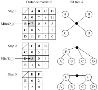
Figure 2 shows an example of the building process of a phylogenetic tree using the Neighbor-Joining method for a 4x4 distance matrix. A B C D A B C D B 7 0 5 8 C 8 5 0 5 D 11 8 5 0 A 0 7 8 11 Step 1 Step 2 C D E D 5 0 6 E 3 6 0 C 0 5 3 A B C D E Step 3 E F F 2 0 E 0 2 A B C D E F
Distance matrix d NJ tree S
Min(Di,j)
Min(Di,j)
Fig. 2 Building process of a phylogenetic tree with the Neighbor-Joining method for a 4x4 distance matrix
IV.PARALLELIZATION OF THE NEIGHBOR-JOINING METHOD A. Sequential Neighbor-Joining Algorithm
The algorithm starts with a distance matrix between pairs of sequences of N
×
N denoted as d, N being the number of sequences. The distance between two sequences can be defined in many ways. The simplest one is known as p-distance and is defined as the ratio between the number of different positions and the total number of positions of the two sequences. Other possibilities are the Jukes-Cantor method or the Kimura method [20]. Since the distance matrixis symmetric, there is no need to store it in full, but only the lower triangular matrix or the upper triangular matrix can be stored (in this case, the former is chosen).
In each iteration of the main loop, the pair i, j for which Di,j is minimal has to be found. The normalized distance
matrix D is not stored, but the value of each position is calculated in each iteration. Node divergences are computed in a one-dimensional array before starting the main loop, and are updated in each iteration of the loop, rather than calculating them every time they are required.
For the list of active nodes L, a one-dimensional flag arrangement is used; the flags indicate which nodes have been selected and which have not.
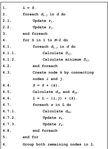
Figure 3 details the pseudo-code of the sequential algorithm. 1. L = S. 2. foreach di,j in d do 2.1. Update ri. 2.2. Update rj. 3. end foreach 4. for h in 1 to N-2 do 4.1. foreach di,j in d do 4.1.1. Calculate Dij. 4.1.2. Calculate minimum Dij. 4.2. end foreach
4.3. Create node k by connecting
nodes i and j. 4.4. S = S + {k}. 4.5. Calculate dik and djk. 4.6. L = L – {i,j} + {k}. 4.7. foreach s in L do 4.7.1. Calculate dks. 4.7.2. Update rk. 4.7.3. Update rs. 4.8. end foreach 5. end for
6. Group both remaining nodes in L.
Fig. 3 Pseudo-code of the sequential algorithm B. Hybrid Parallel Neighbor-Joining Algorithm
The algorithm was parallelized using a master-slave model with a hybrid communication model (combination of
message passing and shared memory). Before going into an in-depth review of the solution developed, certain aspects of the Neighbor-Joining algorithm should be analyzed, since these might explain why an efficient parallel solution is difficult to obtain.
First, it should be noted that for each iteration of the main loop, a new node is added to the distance matrix, but those from the two originating nodes are removed. This means that, in a parallel solution, the work carried out by each task in each iteration decreases as the iterations of the main loop progress. Also, in distributed environments, the distances of the new nodes must be distributed among all processes forming the solution.
The search for the pair of nodes whose distance is minimal represents the most expensive part of the main loop from a computational standpoint. Taking into account that the distance matrix is triangular, distributing the work required for the search process by assigning the same number of rows to each task could result into idle time, since not all rows have the same number of cells. Since idle time negatively affects the performance of an algorithm, it must be removed or, if this is not possible, minimized. For this reason, the workload distribution strategy must be chosen trying to make it as equitable as possible for all tasks.
1. The master process divides distance
matrix d into P portions and distributes
P-1 among the slaves. Each process keeps
approximately ((N)x(N-1)/2P) elements
from distance matrix d.
2. Each process calculates the partial divergences of the nodes it has,
broadcasts them to the other processes, and updates its divergence vector based on the partial divergences received from the other processes.
3. for h in 1 to N-2 do
3.1. Each process calculates its local
minimum Di,j
3.2. The master process collects all
local minimums, calculates the
global minimum Di,j, and broadcasts
it to the other processes.
3.3. The master process creates a new
node k and adds it to S.
3.4. The process owner of node k
calculates dik and djk. Each
remaining process accumulates in a data structure the distances to the
pair of nodes i,j it has and then
sends it to the owner process of
node k.
3.5. The owner process of node k
calculates the distances from it to the rest of the nodes and updates the divergence vector.
3.6. The owner process of node k
broadcasts to the other processes the updated divergence vector.
3.7. Each process removes nodes i and j
from their own L and add k.
3.8. end for
Fig. 4 Pseudo-code of the parallel algorithm
Distance matrix
0
0
0
0
0
0
0
0
0
0
Processes ThreadsN
N
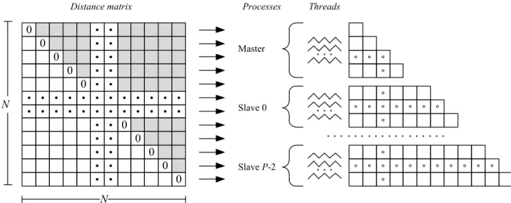
Slave 0 Master Slave P-2Fig. 5 Resolution scheme used by the parallel algorithm of an N×N distance matrix with P processes As it was mentioned, this solution uses a master-slave
model of P processes as parallelization strategy. Each process generates T threads when computation begins. Then, the iterations belonging to different process loops are distributed among the threads that have been generated. The distances of each newly created node are distributed among all processes following a circular order (the node to which it is assigned is the owner).
Figure 4 details the pseudo-code of the parallel algorithm and Figure 5 shows the resolution scheme used by it for an N×N distance matrix with P processes.
V. EXPERIMENTAL WORK A. Architecture Used
Tests were carried out on a cluster of Blade multicores with four blades and two quad core Intel Xeon e5405 2.0 GHz processors each. Each blade has 10 Gb RAM memory (shared between both processors) and 2 x 6Mb L2 cache for each pair of cores. The operating system is GNU/Linux Fedora 12.
Figure 6 shows a schematic representation of the architecture used. Interconnection network Multicore Processor Memory Multicore Processor Memory Multicore Processor Memory Multicore Processor Memory Multicore Processor Multicore
Processor Multicore Processor
Core 0 Core 1 L1 Cache L1 Cache L2 Cache Core 2 Core 3 L1 Cache L1 Cache L2 Cache Multicore Processor
Fig. 6 Schematic representation of the architecture used. B. Algorithms Used
The algorithms used in this work were developed using C language (gcc compiler version 4.4.2) with the OpenMPI
library (mpicc compiler version 1.4.3) for message passing and OpenMP for thread management [14][15]. The sequential
algorithm is based on the solution presented in Section IV.A, while the parallel algorithm is based on the solution described in Section IV.B, P being the number of blades used and T being the number of cores in each blade.
C. Tests Carried Out
Based on the features of the architecture, the parallel algorithm was tested using all the cores with different numbers of nodes: two, three and four; this means that 16, 24 and 32 cores were used, respectively. Each process was mapped to a different node. Various problem sizes were used: N = {4000, 6000, 8000, 10000, 12000, 14000, 16000} and synthetic data sets were employed in the tests. Each particular test was run five times, and the average execution time was calculated for each of them.
VI.RESULTS
To assess the behavior of the algorithms developed when escalating the problem and/or the architecture, the speedup and efficiency of the tests carried out are analyzed [12] [21] [22].
The speedup metric is used to analyze the algorithm performance in the parallel architecture as indicated in Equation (1). me ParallelTi Time Sequential Speedup = (1)
To assess how good the speedup obtained is, the efficiency metric is calculated. Equation (2) indicates how to calculate this metric, where p is the total number of cores used.
p Speedup
Efficiency= (2)
Table I shows the speedup obtained with the parallel algorithm for the various tested problem sizes when using two, three, and four nodes of the architecture involving 16, 24 and 32 cores, respectively. Figure 7 is a chart representation of those same values.
TABLE I SPEEDUP OBTAINED WITH THE PARALLEL ALGORITHM FOR VARIOUS PROBLEM SIZES USING DIFFERENT NUMBERS OF CORES OF THE
ARCHITECTURE
Problem size Cores of the architecture 16 24 32 4000 7,02 7,09 7,28 6000 8,48 9,57 9,84 8000 9,13 10,78 11,57 10000 9,66 11,87 13,11 12000 10,07 12,65 14,32 14000 10,32 13,12 15,15 16000 10,57 13,80 16,00
Fig. 7 Speedup obtained with the parallel algorithm for various problem sizes using different numbers of cores of the architecture
Based on the previous chart, it can be said that the parallel algorithm has a good performance, achieving a 16-fold reduction of the execution time of the sequential algorithm. It can also be seen that the speedup escalates as the size of the problem increases.
Table 2 shows the efficiency obtained with the parallel algorithm for the various tested problem sizes when using two, three, and four nodes of the architecture involving 16, 24 and 32 cores, respectively. Figure 8 is a chart representation of those same values.
The previous chart shows that efficiency increases as the size of the problem increases, and that, on the other hand, it decreases as the number of nodes used increases. It can be said that the efficiency levels obtained by the parallel algorithm are good considering the large number of communications and synchronization operations carried out and the idle time that one or more threads in each process could have due to the characteristics of the problem.
Section II described related works. A comparative analysis with them would be useful to appreciate the results obtained in this work. Unfortunately, not all of them can be compared. The Pthreads algorithm presented in the Sahoo, Behura and Padhy work [17] was tested using small numbers
of sequences and processors, making impossible to include it in the analysis. The CUDA algorithm [18] developed by Liu,
Schmidt and Maskell is excluded from the comparison for using a too different architecture and technology. Bullard declares in his work [3] that his sequential implementation
was not “optimized”, so including his parallel algorithm in the comparison would be unfair. Finally, Du and Lin [16] used
similar support architecture and technologies, so the comparative analysis is made with their algorithm.
TABLE II EFFICIENCY OBTAINED WITH THE PARALLEL ALGORITHM FOR VARIOUS PROBLEM SIZES USING DIFFERENT NUMBERS OF CORES OF THE
ARCHITECTURE
Problem size Cores of the architecture 16 24 32 4000 0,44 0,30 0,23 6000 0,53 0,40 0,31 8000 0,57 0,45 0,36 10000 0,60 0,49 0,41 12000 0,63 0,53 0,45 14000 0,65 0,55 0,47 16000 0,66 0,57 0,50
Fig. 8 Efficiency obtained with the parallel algorithm for various problem sizes using different numbers of cores of the architecture
Fig. 9 Speedup achieved by the algorithm of Du and Lin and the algorithm presented in this work when using different number of processing units of
the support architecture for N=10000
Figure 9 shows the speedup achieved by the algorithm of Du and Lin and the algorithm presented in this work when using different number of processing units of the support architecture for N=10000.
From this last chart, it can be seen that the algorithm presented in this work obtains higher speedup values compared to the algorithm of Du and Lin. This fact confirms the good performance achieved by the first.
VII. CONCLUSIONS AND FUTURE WORKS
Building phylogenetic trees following the Neighbor-Joining method is an application with a high computational
demand, which makes parallel processing appropriate to speed it up. In this paper, we have presented a hybrid parallel algorithm to be run on current cluster architectures.
The experimental results obtained show that speedup increases with the size of the problem, with a greater slope when more cores are used. Time is reduced up to 16 times when using all the cores of the support architecture for the largest problem size. At the same time, efficiency also increases with N, although naturally (due to the communication overhead), the greatest efficiency is achieved with 16 cores.
Some of the possible future lines of work are:
•analyzing other possible distance distribution strategies for the new nodes that are added to the tree in order to improve load balancing among the processes.
•analyzing scalability in detail when increasing the problem size and the number of cores used.
•designing other types of hybrid solutions combining multicore processors and GPUs.
REFERENCES
[1] R. Durbin, S.R. Eddy, A. Krogh, and G.J. Mitchison, Biological Sequence Analysis: Probabilistic Models of Proteins and Nucleic Acids, Cambridge University Press, UK, 1998.
[2] T.K. Attwood, D.J. Parry-Smith, Introducción a la Bioinformática, Pearson Education S.A, 2002.
[3] J. Bullard, “panjo: a parallel neighbor joining algorithm”, University of California, Berkeley, Tech. Rep., 2007.
[4] (2012) Clustal W, Clustal X Multiple Sequence Alignment. [Online]. Available at http://www.clustal.org/clustal2/. [5] N. Saitou, M. Nei, “The neighbor-joining method: a new
method for reconstructing phylogenetic trees”, Mol. Biol. Evol., vol. 4, pp. 406-425, 1987.
[6] J.A. Studier, K.J. Keppler, “A note on the neighbour-joining algorithm of Saitou and Nei”, Mol. Biol. Evol., vol. 5, pp. 729-731, 1988.
[7] G. Moore, “Cramming more components onto integrated circuits”, Electronics, vol. 38, no. 9, pp. 82-85, Apr. 1965. [8] (2009) Multi-Core Technology Evolution. [Online]. Available
at http://multicore. amd.com/es-ES/AMD-Multi-Core/resources/Technology-Evolution.
[9] (2010) Intel Multi-Core Processors: Quick Reference Guide.
[Online]. Available at http://cachewww.intel.com/cd/00/00/23/19/231912_231912.p
df.
[10] M. McCool, “Scalable Programming Models for Massively Parallel Multicores”, Proceedings of the IEEE, vol. 96, no. 5, pp. 816–831, 2008.
[11] (2012) Cluster and Grid Computing course @ University of Melbourne. [Online]. Available at http://www.cs.mu.oz.au/678/.
[12] Z. Juhasz, P. Kacsuk, and D. Kranzlmuller, Distributed and Parallel Systems: Cluster and Grid Computing, Springer, USA, 2004.
[13] L. Chai, Q. Gao, D.K. Panda, “Understanding the impact of multi-core architecture in cluster computing: A case study with Intel Dual-Core System”, in Proc of the. IEEE International Symposium on Cluster Computing and the Grid 2007 (CCGRID 2007), pp. 471-478, May 2007.
[14] (2012) OpenMP: The OpenMP API specification for parallel programming. [Online]. Available at http://www.openmp.org. [15] (2012) OpenMPI: Open Source High Performance Computing.
[Online]. Available at http://www.open-mpi.org.
[16] Z. Du, F. Lin, “pNJTree: A parallel program for reconstruction of neighbor-joining tree and its application in ClustalW”, Parallel Computing, vol. 32, no. 5, pp. 441-446, 2006.
[17] B. Sahoo, A. Behura and S. Padhy, “Fine Grain Construction of Neighbour-Joining Phylogenetic Tress with Reduced Redundancy Using Multithreading”, International Journal of Distributed and Parallel Systems (IJDPS), vol. 1, no. 2, pp. 129-140, 2010.
[18] Y. Liu, C. Schmidt and D. L. Maskell, “Parallel reconstruction of neighbor-joining trees for large multiple sequence alignments using CUDA”, Proc. of the IPDPS '09 Proceedings of the 2009 IEEE International Symposium on Parallel & Distributed Processing, pp. 1-8, 2009.
[19] (2012) Parallel Programming and Computing Platform | CUDA | NVIDIA. [Online]. Available at http://www.nvidia.com/object/cuda_home_new.html.
[20] (2012) T. Speed. Statistical Genetics. Course material. Department of Statistics, University of California at Berkeley.
Available at http://www.stat.berkeley.edu/users/terry/Classes/s246.2006/W
eek6/2neighbourJoining.pdf.
[21] A. Grama, A. Gupta, G. Karypis and V. Kumar, An introduction to parallel computing. Design and analysis of algorithms, 2nd ed., Addison Wesley, England, 2003. [22] B. Wilkinson, M. Allen, Parallel programming. Techniques
and Applications using networked workstations and parallel computers, 2nd ed., Prentice Hall, USA, 2005.
Enzo Rucci has a B.Sc. in Computer Science from the National University of La Plata (Argentina) and is a Doctorate student of Computer Science at that same University. His area of interest is parallel and distributed processing.
He has published articles in several national and international congresses and journals in areas related to parallel and distributed processing, as well as bioinformatics.
Franco Chichizola has a B.Sc. in Computer Science from the National University of La Plata (Argentina) and is a Doctorate student of Computer Science at that same University. His area of interest is parallel and distributed processing.
He is currently an Associate Professor at the School of Computer Science of the National University of La Plata, Argentina. He has published articles in several congresses and journals in areas related to parallel and distributed processing, as well as bioinformatics.
Marcelo Naiouf has a B.Sc. in Computer Science from the National University of La Plata (Argentina) and a PhD in Computer Science at that same University. His area of interest is parallel and distributed processing.
He is currently Head Professor at the School of Computer Science of the National University of La Plata, Argentina. He has published articles in several congresses and journals in areas
related to parallel and distributed processing, as well as bioinformatics.
Armando E. De Giusti is a Telecommunications Engineer from the National University of La Plata (Argentina) with Specialization in Computer Sciences Applied to Education at that same University. His areas of interest are parallel and distributed processing and computer science applied to education.
He is currently Head Professor at the School of Computer Science of the National University of La Plata (Argentina) and Principal Investigator of the CONICET. He has authored several books and has articles in several congresses and journals in areas related to parallel and distributed processing, as well as bioinformatics.