Variational Inference for Sparse Gaussian Process Modulated Hawkes Process

Variational Inference for Sparse Gaussian Process Modulated Hawkes Process

Rui Zhang,

_{Christian Walder,}

_{Marian-Andrei Rizoiu}

Abstract

The Hawkes process (HP) has been widely applied to model-ing self-excitmodel-ing events includmodel-ing neuron spikes, earthquakes and tweets. To avoid designing parametric triggering kernel and to be able to quantify the prediction confidence, the non-parametric Bayesian HP has been proposed. However, the inference of such models suffers from unscalability or slow convergence. In this paper, we aim to solve both problems. Specifically, first, we propose a new non-parametric Bayesian HP in which the triggering kernel is modeled as a squared sparse Gaussian process. Then, we propose a novel varia-tional inference schema for model optimization. We employ the branching structure of the HP so that maximization of evidence lower bound (ELBO) is tractable by the expectation-maximization algorithm. We propose a tighter ELBO which improves the fitting performance. Further, we accelerate the novel variational inference schema to linear time complexity by leveraging the stationarity of the triggering kernel. Different from prior acceleration methods, ours enjoys higher efficiency. Finally, we exploit synthetic data and two large social media datasets to evaluate our method. We show that our approach outperforms state-of-the-art non-parametric frequentist and Bayesian methods. We validate the efficiency of our acceler-ated variational inference schema and practical utility of our tighter ELBO for model selection. We observe that the tighter ELBO exceeds the common one in model selection.

1

Introduction

The Hawkes process (HP) (Hawkes 1971) is particularly useful to model self-exciting point data – i.e., when the occur-rence of a point increases the likelihood of occuroccur-rence of new points. The process is parameterized using a background in-tensityµ, and a triggering kernelφ. The Hawkes process can be alternatively represented as a cluster of Poisson processes (PPes) (Hawkes and Oakes 1974). In the cluster, a PP with an intensityµ(denoted as PP(µ)) generates immigrant points which are considered to arrive in the system from the outside, and every existing point triggers offspring points, which are generated internally through the self-excitement, following a PP(φ). Points can therefore be structured into clusters where each cluster contains either a point and its direct offspring or the background process (an example is shown in Fig. 1a). Connecting all points using the triggering relations yields

Copyright c2020, Association for the Advancement of Artificial Intelligence (www.aaai.org). All rights reserved.

(a) Poisson Cluster Process (b) Branching Structure

Figure 1: The Cluster Representation of a HP. (a) A HP with a decaying triggering kernelφ(_·)has intensityλ(x)which increases after each new point (dash line) is generated. It can be represented as a cluster of PPes: PP(µ) and PP(φ(x₋ xi)) associated with eachxi. (b) The branching structure

corresponding to the triggering relationships shown in (a), where an edgexi →xjmeans thatxitriggersxj, and its

probability is denoted aspji.

a tree structure, which is called the branching structure (an example is shown in Fig. 1b corresponding to Fig.1a). With the branching structure, we can decompose the HP into a cluster of PPes. The triggering kernelφis shared among all cluster Poisson processes relating to a HP, and it determines the overall behavior of the process. Consequently, designing the kernel functions is of utmost importance for employing the HP to a new application, and its study has attracted much attention.

Prior non-parametric frequentist solutions.In the case in which the optimal triggering kernel for a particular ap-plication is unknown, a typical solution is to express it us-ing a non-parametric form, such as the work of Lewis and Mohler (2011); Zhou, Zha, and Song (2013); Bacry and Muzy (2014); Eichler, Dahlhaus, and Dueck (2017). These are all frequentist methods and among them, the Wiener-Hoef equation based method (Bacry and Muzy 2014) en-joys linear time complexity. Our method has a similar ad-vantage of linear time complexity per iteration. The Euler-Lagrange equation based solutions (Lewis and Mohler 2011; Zhou, Zha, and Song 2013) require discretizing the input

domain so they face a problem of poorly scaling with the dimension of the domain. The same problem is also faced by Eichler, Dahlhaus, and Dueck (2017)’s discretization based method. In contrast, our method requires no dixscretization so enjoys scalability with the dimension of the domain.

Prior Bayesian solutions. The Bayesian inference for the HP has also been studied, including the work of Ras-mussen (2013); Linderman and Adams (2014); Linder-man and Adams (2015). These work require either con-structing a parametric triggering kernel (Rasmussen 2013; Linderman and Adams 2014) or discretizing the input domain to scale with the data size (Linderman and Adams 2015). The shortcoming of discretization is just mentioned and to over-come it, Donnet, Rivoirard, and Rousseau (2018) propose a continuous non-parametric Bayesian HP and resort to an unscalable Markov chain Monte Carlo (MCMC) estimator to the posterior distribution. A more recent solution based on Gibbs sampling (Zhang et al. 2019) obtains linear time complexity per iteration by exploiting the HP’s branching structure and the stationarity of the triggering kernel similar to the work of Halpin (2012). This approach considers only high-probability triggering relationships in computations for acceleration. However, those relationships are updated in each iteration, which is less efficient than our pre-computing them. Besides, our variational inference schema enjoys faster convergence than that of the Gibbs sampling based method.

Contributions.In this paper, we propose the first sparse Gaussian process modulated HP which employs a novel vari-ational inference schema, enjoys a linear time complexity per iteration and scales to large real world data. Our method is inspired by the variational Bayesian PP (VBPP) (Lloyd et al. 2015) which provides the Bayesian non-parametric inference only for the whole intensity of the HP without for its compo-nents: the background intensityµand the triggering kernelφ. Thus, the VBPP loses the internal reactions between points, and developing the variational Bayesian non-parametric infer-ence for the HP is non-trivial and more challenging than the VBPP. In this paper, we adapt the VBPP for the HP and term the new approach the variational Bayesian Hawkes process (VBHP). The contributions are summarized:

(1)(Sec.3) We introduce a new Bayesian non-parametric HP which employs a sparse Gaussian process modulated trig-gering kernel and a Gamma distributed background intensity.

(2) (Sec.3&4) We propose a new variational inference schema for such a model. Specifically, we employ the branch-ing structure of the HP so that maximization of the evi-dence lower bound (ELBO) is tractable by the expectation-maximization algorithm, and we contribute a tighter ELBO which improves the fitting performance of our model.

(3) (Sec.5) We propose a new acceleration trick based on the stationarity of the triggering kernel. The new trick enjoys higher efficiency than prior methods and accelerates the variational inference schema to linear time complexity per iteration.

(4)(Sec.6) We empirically show that VBHP provides more accurate predictions than state-of-the-art methods on syn-thetic data and on two large online diffusion datasets. We validate the linear time complexity and faster convergence of our accelerated variational inference schema compared to

the Gibbs sampling method, and the practical utility of our tighter ELBO for model selection, which outperforms the common one in model selection.

2

Prerequisite

In this section, we review the Hawkes process, the variational inference and its application to the Poisson process.

2.1

Hawkes Process (HP)

The HP (Hawkes 1971) is a self-exciting point process, in which the occurrence of a point increases the arrival rateλ(_·), a.k.a. the (conditional) intensity, of new points. Given a set of time-ordered points_D=_{xi}iN=1,xi∈RR, the intensity

atxconditioned on given points is written as: λ(x) =µ+ X

xi<x

φ(x₋xi),

whereµ > 0 is a constant background intensity, and φ :

RR→[0,∞)is the triggering kernel.

We are particularly interested in the branching structure of the HP. As introduced in Sec.1, each pointxihas a parent that

we represent by a one-hot vectorbi= [bi0, bi1,· · ·, bi,i−1]T:

each element bij is binary,bij = 1represents that xi is

triggered byxj (0≤j ≤i−1,x0: the background), and

Pi−1

j=0bij = 1. A branching structureBis a set ofbi, namely

B=_{bi}Ni=1, and if the probability ofbij= 1is defined as

pij ≡p(bij = 1), the probability ofBcan be expressed as

p(B) =QN

i=1

Qi−1

j=0p

bij

ij . Sincebiis a one-hot vector, there

isPi−1

j=0pij = 1for alli.

Given both_Dand a branching structureB, the log like-lihood of µ and φ becomes a sum of log likelihoods of PPes. With B, the HP _Dcan be decomposed into PP(µ) and_{PP(φ(x₋xi))}Ni=1. The data domain of PP(µ) equals

that of the HP, which we denote_T, and we denote the data domain of PP(φ(x₋xi)) byTi ⊂ T. As a result, the log

likelihoodlogp(D, B_|µ, φ)is expressed as: logp(_D,B_|µ,φ)= N X i=1 Xi−1 j=1 bijlogφij+bi0logµ − N X i=1 Z Ti φ₋µ_{|T |}, (1) where _{|T | ≡} R T 1dx, φij ≡ φ(xi −xj) and R Tiφ ≡ R

Tiφ(x)dx. Throughout this paper, we simplify the

integra-tion by omitting the integraintegra-tion variable, which isxunless otherwise specified. This work is developed based on the univariate HP. However, it can be extended to be multivariate following the same procedure.

2.2

Variational Inference (VI)

Consider the latent variable modelp(x,z_|θ)wherexandz

are the data and the latent variables respectively. The vari-ational approach introduces a varivari-ational distribution to ap-proximate the posterior distributionq(z_|θ0)_≈p(z_|x,θ)and maximizes a lower bound of the log-likelihood, which can be derived from the non-negative gap perspective:

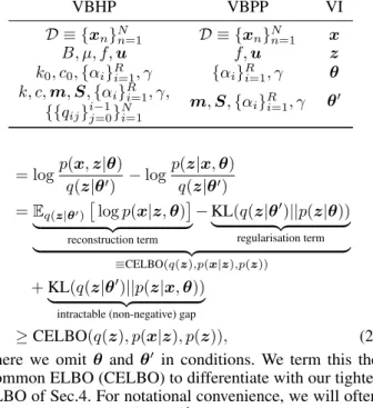
Table 1: Notations VBHP VBPP VI D ≡ {xn}Nn=1 D ≡ {xn}Nn=1 x B, µ, f,u f,u z k0, c0,{αi}Ri=1, γ {αi}Ri=1, γ θ k, c,m,S,_{αi}Ri=1, γ, _m,S, {αi}Ri=1, γ θ0 {{qij}ij−=01} N i=1 = logp(x,z|θ) q(z_|θ0₎ −log p(z_|x,θ) q(z_|θ0₎ =Eq(z|θ0₎logp(x|z,θ) | {z } reconstruction term −KL(q(z_|θ0)_||p(z_|θ)) | {z } regularisation term | {z } ≡CELBO(q(z),p(x|z),p(z)) +KL(q(z_|θ0)_||p(z_|x,θ)) | {z }

intractable (non-negative) gap

≥CELBO(q(z), p(x_|z), p(z)), (2) where we omit θ and θ0 in conditions. We term this the Common ELBO (CELBO) to differentiate with our tighter ELBO of Sec.4. For notational convenience, we will often omit conditioning onθandθ0 hereinafter. Optimizing the CELBO w.r.t.θ0balances between the reconstruction error and the Kullback-Leibler (KL) divergence from the prior. Generally, the conditionalp(x_|z)is known, so is the prior. Thus, for an appropriate choice ofq, it is easier to work with this lower bound than with the intractable posteriorp(z_|x). We also see that, due to the form of the intractable gap, if qis from a distribution family containing elements close to the true unknown posterior, thenqwill be close to the true posterior when the CELBO is close to the true likelihood. An alternative derivation applies Jensen’s inequality (Jordan et al. 1999).

2.3

Variational Bayesian Poisson Process (VBPP)

VBPP (Lloyd et al. 2015) applies the VI to the Bayesian Poisson process, which exploits the sparse Gaussian process (GP) to model the Poisson intensity. Specifically, VBPP uses a squared link function to map a sparse GP distributed func-tionf to the Poisson intensityλ(x) =f2(x). The sparse GP employs the ARD kernel:

K(x,x0)_≡γ R Y r=1 exp₋(xr−x 0 r) 2 2αr .

where γand _{αr}Rr=1are GP hyper-parameters. Letu ≡

(f(z1), f(z2),· · · , f(zM)) where zi are inducing points.

The prior and the approximate posterior distributions of

u are Gaussian distributions p(u) = _N(u_|0,Kzz) and

q(u) = _N(u_|m,S)wheremandSare the mean vector and the covariance matrix respectively. Note bothuandf employ zero mean priors. Notations of VBPP are connected with those of VI (Sec.2.2) in Table1.

Importantly, the variational joint distribution off andu

uses the exact conditional distributionp(f_|u), i.e.,

q(f,u)_≡p(f_|u)q(u) (3)

which in turn leads to the posterior GP:

q(f) =_N(f_|ν,Σ), (4) ν(x)_≡KxzKzz−1m,

Σ(x,x0)_≡Kxx0+K_xzK_zz−1(SK_zz−1−I)K_zx0.

Then, the CELBO is obtained by using Eqn.(2): CELBO(q(f,u), p(_D|f,u), p(f,u))

=_Eq(f)[logp(D|f)]−KL(q(u)||p(u)).

Note that the second term is the KL divergence between two multivariate Gaussian distributions, so is available in closed form. The first term turns out to be the expectation w.r.t.q(f) of the log-likelihoodlogp(_D|f) =PN

i=1logf 2_(x

i)−R_Tf2.

The expectation of the integral part is relatively straight-forward to compute and the expectation of the other (data-dependent) part is available in almost closed-form with a hyper-geometric function.

3

Variational Bayesian Hawkes Process

3.1

Notations

To extend VBPP to HP, we introduce two more variables: the background intensityµand the branching structureB, defined in Sec.2.1. We assume that the prior distribution of µis a Gamma distributionp(µ) = Gamma(µ_|k0, c0)1 and

the posterior distribution is approximated by another Gamma distributionq(µ) =Gamma(µ_|k, c). ForB=_{bi}Ni=1given

D=_{xi}Ni=1, we assume the variational posteriorbij,j=

0,_{· · ·} , i₋1, have a categorical distribution:qij =q(bij =

1)and Pi−1

j=0qij = 1, and thus, the variational posterior

probability ofBis expressed as: q(B) = N Y i=1 i−1 Y j=0 qbij ij . (5)

The same squared link function is adopted for the trig-gering kernelφ(x) =f2_{(x), so are the priors forf andu,}

namely_N(f_|0,Kxx0)andN(u|0,K_zz0). More link

func-tions such asexp(_·)are discussed by Lloyd et al. (2015). Moreover, we use the same variational joint posterior onf anduas Eqn.(3). Consequently, we complete the variational joint distribution on all latent variables as below:

q(B,µ,f,u)_≡q(B)q(µ)p(f_|u)q(u), (6) and notations of VBHP are summarized in Table 1.

3.2

CELBO

Based on Eqn.(2)&(6), we obtain the CELBO for VBHP (see details in A.1 of the appendix (App. 2019)):

CELBO(q(B, µ, f,u), p(_D|B, µ, f,u), p(B, µ, f,u)) =Eq(B,µ,f)

h

logp(_D, B_|f, µ)i

| {z }

Data Dependent Expectation (DDE) +HB 1_Gamma(µ|k 0, c0) = 1 Γ(k0)ck0 µk0−1_e−x/c0

−KL(q(µ)_||p(µ))₋KL(q(u)_||p(u)). (7) whereHB =−PN_i=1P_ji−₌₀1qijlogqijis the entropy of the

variational posteriorB. The KL terms are between gamma and Gaussian distributions for which closed forms are pro-vided in A.2 of the appendix (App. 2019).

3.3

Data Dependent Expectation

Now, we are left with the problem of computing the data dependent expectation (DDE) in Eqn.(7). The DDE is w.r.t. the variational posterior probabilityq(B, µ, f). From Eqn.(6), q(B, µ, f) =R

q(B, µ, f,u)du=q(B)q(µ)q(f)andq(f) is identical to Eqn.(4). As a result, we can compute the DDE w.r.t.q(B)first, and then w.r.t.q(µ)andq(f).

Expectation w.r.t.q(B).From Eqn.(1), we easily obtain logp(_D, B_|f, µ)by replacingφ withf2_{, whereupon it is}

clear that only bij inlogp(D, B|f, µ)is dependent onB.

Therefore,Eq(B)[logp(D, B|f, µ)]is computed as:

Eq(B)[logp(D,B|f,µ)] = N X i=1 _Xi−1 j=1 qijlogfij2+qi0logµ − N X i=1 Z Ti f2₋µ_{|T |} wherefij ≡f(xi−xj).

Expectation w.r.t.q(f) andq(µ).We compute the ex-pectation w.r.t. q(f) and q(µ) by exploiting the expecta-tion and the log expectaexpecta-tion of the Gamma distribuexpecta-tion:

Eq(µ)(µ) =kcandEq(µ)(log(µ)) =ψ(k) + logc, and also

the propertyE(x2) =E(x)2+Var(x):

DDE= N X i=1 hXi−1 j=1 qijEq(f)(logfij2)+qi0 ψ(k)+logc − Z Ti E2q(f)(f)− Z Ti Varq(f)(f) i −kc_{|T |}, (8) whereψis the Digamma function. We provide closed form expressions for R TiE 2 q(f)(f) and R TiVarq(f)(f) in A.3 of

the appendix (App. 2019). As in VBPP,_Eq(f)(logfij2) =

−Ge(−ν_ij2/(2Σij))+log(Σij/2)−Cis available in the closed

form with a hyper-geometric function, whereνij =ν(xi−

xj),Σij = Σ(xi−xj,xi−xj)(ν andΣare defined in

Eqn.(4)),C_≈0.57721566is the Euler-Mascheroni constant andGe is defined asGe(z) = ₁F

(1,0,0)

1 (0,1/2, z), i.e., the

partial derivative of the confluent hyper-geometric function

1F1w.r.t. the first argument. We computeGeusing the method of Ancarani and Gasaneo (2008) and implementG˜ andG˜0 by linear interpolation of a lookup table (see a demo in the supplementary material).

3.4

Predictive Distribution of

φ

The predictive distribution off(x)depends on the poste-rioru. We assume that the optimal variational distribution ofuapproximates the true posterior distribution, namely q(u_|D,θ0∗) =_N(u_|m∗,S∗)_≈p(u_|D,θ). Therefore, there is q(f_|D,θ0∗) _≈ p(f_|D,θ), i.e., the approximate predic-tive f( ˜x) _{∼ N}(Kxz˜ Kzz−1m∗,Kx˜x˜ − K˜xzKzz−10Kzx˜ +

K˜xzKzz−10S∗K−

1

zz0Kz˜x)≡ N(˜ν,σ˜2). Given the relationφ=

f2, it is straightforward to derive the correspondingφ( ˜x)_∼ Gamma(˜k,c˜)where the shape˜k= (˜ν2+ ˜σ2)2/[2˜σ2(2˜ν2+ ˜

σ2_{)]and the scale˜c= 2˜σ}2_(2˜ν2_{+ ˜σ}2_)/(˜ν2_{+ ˜σ}2_).

4

New Variational Inference Schema

Theorem 1. For VBHP, there is a tighter ELBO

Eq(B,µ,f) h logp(_D, B_|f, µ)i+HB | {z } ≡TELBO ≤logp(_D). Remark. TELBO is tighter because it is equivalent to the CELBO (Eqn.(7)) except without subtracting non-negative KL divergences overµandu. Other graphical models such as the variational Gaussian mixture model (Attias 1999) have a similar TELBO. Later on, we propose a new VI schema based on the TELBO.

Proof. With the variational posterior probability of the branching structure q(B) defined in Eqn.(5) and through the Jensen’s inequality, we have:

logp(_D)_≥X

B

q(B) logp(_D, B) +HB, (9)

whereHBis the entropy ofBdefined in Eqn.(7). The term

P

Bq(B) logp(D, B)can be understood as follows.

Con-sider that infinite branching structures are drawn fromq(B) independently, say_{Bi}∞i=1. Given a branching structureBi,

the Hawkes process can be decomposed into a cluster of Pois-son processes, denoted as (_D, Bi), and the corresponding

log-likelihood islogp(_D, Bi). Then,PBq(B) logp(D, B)

is the mean of all log likelihoods_{logp(_D, Bi)}∞i=1,

lim n→∞ 1 n n X i=1 logp(_D, Bi) = lim n→∞ X B nB n logp(D, B) =X B q(B) logp(_D, B), (10) wherenB is the number of occurences of branching

struc-tureB. Since all branching structures_{Bi}∞i=1are i.i.d., the

clusters of Poisson processes generated over_{Bi}∞i=1should

also be independent, i.e.,_{(_D, Bi)}∞i=1are i.i.d.. It follows

that

∞

X

i=1

logp(_D, Bi) = logp({(D, Bi)}∞i=1). (11)

We compute the CELBO oflogp(_{(_D, Bi)}∞i=1)by making

z= (µ, f,u)andx=_{(_D, Bi)}ni=1in Eqn.(2):

logp(_{(_D,Bi)}ni=1)≥Eq(f,µ)

logp(_{(_D,Bi)}ni=1|f,µ)]

−KL(q(µ)_||p(µ))₋KL(q(u)_||p(u)). (12) Further, we plug Eqn.(11) and Eqn.(12) into Eqn.(10):

Eqn.(10)= lim n→∞ 1 nlogp({(D, Bi)} n i=1)

(a) ≥ lim n→∞ 1 nEq(f,µ) logp(_{(_D, Bi)}ni=1|f, µ)] (b) = lim n→∞ X nB nB n Eq(f,µ) logp(_D, B_|f, µ) =Eq(f,µ,B) logp(_D, B_|f, µ)

where (a) is because the finite values of KL terms are divided by infinitely largen, and (b) is due to i.i.d.(_D, Bi)and the

variational posteriorBbeing independent offandµ. Finally, we plug the above inequality into Eqn.(9) and obtain the TELBO.

New Optimization Schema for VBHP To optimize the model parameters, we employ the expectation-maximization algorithm. Specifically, in theE step, allqij are optimized to

maximize the CELBO, and in theM step,m,S,kandcare updated to increase the CELBO. We don’t use the TELBO to optimize the variational distributions because it doesn’t guar-antee minimizing the KL divergence between variational and true posterior distributions. Instead, the TELBO is employed to select GP hyper-parameters:

{α∗_i}R_i=1, γ∗=argmax_{α

i}Ri=1,γTELBO.

The TELBO bounds the marginal likelihood more tightly than CELBO, and is therefore expected to lead to a better predictive performance — an intuition which we empirically validate in Sec.6.

The updating equations forqijare derived through

maxi-mization of Eqn.(7) under the constraintsPi−1

j=0qij= 1for

alli. This maximization problem is dealt with the Lagrange multiplier method, and yields the below updating equations:

qij = _exp( Eq(f)(logfij2))/Ai, j >0; θexp(ψ(k))/Ai, j= 0, whereAi=θexp(ψ(k)) +P i−1

j=1exp(Eq(f)(logfij2))is the

normalizer.

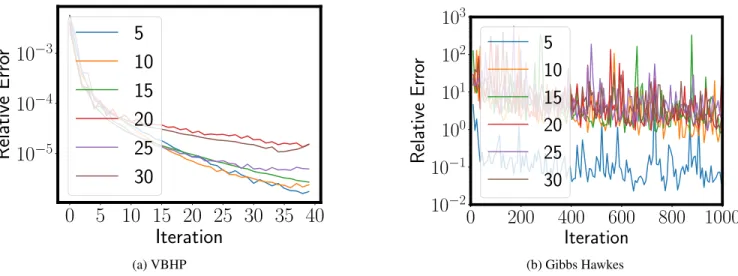
Furthermore, and similarly to VBPP, we fix the inducing points on a regular grid over_T. Despite the observation that more inducing points lead to better fitting accuracy (Lloyd et al. 2015; Snelson and Ghahramani 2006), in the case of our more complex VBHP, more inducing points may cause slow convergence (Fig.5a (App. 2019)) for some hyper-parameters, and therefore lead to poor performance in limited iterations. Generally, more inducing points improve accuracy at the expense of longer fitting time.

5

Acceleration Trick

Time Complexity Without Acceleration In the E step of model optimization, updating qij requires computing

the mean and the variance of all fij, which both take

O(M3+M2N2)withN points in the HP andM induc-ing points. Here, we omit the dimension of dataR since normallyM > Rfor a regular grid of inducing points. Sim-ilarly, in the M step, computing the hyper-geometric term requires the means and variances of all thefij. Finally,

com-putation of the integral terms takesO(M3_{N). Thus, the total}

time complexity per iteration isO(M3N+M2N2).

Acceleration to Linear Time Complexity To accelerate our VBHP, similarly to Zhang et al. (2019) we exploit the stationarity of the triggering kernel, assuming the kernel has negligible values for sufficiently large inputs. As a result, sufficiently distant pairs of points do not enter into the com-putations. This trick reduces possible parents of a point from all prior points to a set of neighbors. The number of relevant neighbors is bounded by a constantCand as a result the total time complexity is reduced toO(CM3_N).

Specifically, we introduce a compact region _S =

×

r=1[Srmin,Srmax]⊆ T so thatφ(xi−xj) = 0andqij = 0

ifxi−xj 6∈ S. As a result, all terms related toxi−xj 6∈ S

vanish. To choose a suitable_S, we again use the TELBO, taking the smallestSfor which the TELBO doesn’t drop sig-nificantly; we optimizeSminr andSmaxr by grid search with

other dimensions fixed (so that this step is runRtimes in total) and we optimizeSmin

r after optimizingSrmax.

Rather than selecting pairs of points in each iteration in the manner of Halpin’s trick (Halpin 2012; Zhang et al. 2019), our method pre-computes those pairs, leading to gains in computational efficiency. The similar aspect is that both tricks have hyper-parameters to select to threshold the triggering kernel value. We employ the TELBO for hyper-parameter selection while frequentist methods use the cross validation.

6

Experiments

Evaluation.We employ two metrics: the first is theL2

dis-tance (for cases with a known ground truth), which mea-sures the difference between predictive and truth Hawkes kernels, formulated as L2(φpred, φtrue) = (R_T(φpred(x)−

φtrue(x))2_dx)0.5_{and L}

2(µpred, µtrue) = |µpred−µtrue|; the

second is the hold-out log likelihood (HLL), which describes how well the predictive model fits the test data, formulated as logp(_DTest ={xi}Ni=1|µ, f) =

PN

i=1logλ(xi)−

R

T λ. To

calculate the HLL for each process, we generate a number of test sequences by every time randomly assigning each point of the original process to either a training or testing sequence with equal probability; HLLs of test sequences are normalized (by dividing test sequence length) and averaged.

Prediction.We use the pointwise mode of the approximate posterior triggering kernel as the prediction because it is computationally intractable to find the posterior mode at multiple point locations (Zhang et al. 2019). Besides, we exploit the mode of the approximate posterior background intensity as the predictive background intensity.

Baselines. We use the following models as baselines.

(1) A parametric Hawkes process equipped with the sum of exponential (SumExp) triggering kernel φ(x) = PK i=1a i 1a i 2exp(−a i

2x)and the constant background

inten-sity.(2)The ordinary differential equation (ODE) based non-parametric non-Bayesian Hawkes process (Zhou, Zha, and Song 2013). The code is publicly available (Bacry et al. 2017).

(3)Wiener-Hopf (WH) equation based parametric non-Bayesian Hawkes process (Zhou, Zha, and Song 2013). The code is publicly available (Bacry et al. 2017).(4)The Gibbs sampling based Bayesian non-parametric Hawkes process (Gibbs Hawkes) (Zhang et al. 2019). For fairness, the ARD kernel is used by Gibbs Hawkes and corresponding

eigenfunc-0.0 0.5 1.0 1.5 2.0 2.5 3.0 Time Difference 0.0 0.5 1.0 1.5 2.0 2.5 T riggering Kernel V alue Gibbs-Hawkes VBHP Truth

(a) Variational Posterior Triggering Kernel

10−2 ₁₀−1 ₁₀0 ₁₀1 α 10−2 10−1 100 101 γ 1100 800 1000 1100 1200 ₁₂₁₆ 1000 (b) TELBO 10−2 ₁₀−1 ₁₀0 ₁₀1 α 10−2 10−1 100 101 γ 0.3 0.7 2.0 3.0 (c) L2 Distance forφ

Figure 2: The Relationship between the Log Marginal Likelihood and the L2Distance. In (a), the trueφsin(dash green) is plotted

with the median (solid) and the [0.1, 0.9] interval (filled) of the approximate posterior triggering kernel obtained by VBHP and Gibbs Hawkes (10 inducing points). It uses the maximum point of the TELBO (red star in (b)). In (c), the maximum point of the TELBO is marked. The maximum point overlaps with that of the CELBO.[0,1.4]is used as the support of the predictive triggering kernel and 10 inducing points are used.

10−2 ₁₀−1 ₁₀0 ₁₀1 α 10−2 10−1 100 101 γ 1.50 2.00 2.40 3.00 3.15 3.29 3.25

(a) Expected TELBO (Train)

10−2 ₁₀−1 ₁₀0 ₁₀1 α 10−2 10−1 100 101 γ 2.40 3.00 3.30 3.34 3.33 3.34 (b) HLL 10 20 30

Number of Inducing Points

0.2 0.3 0.4 0.5 Gibbs Hawkes VBHP 5 10 15

(c) Time VS Inducing Points (d) Time VS Data Size

Figure 3: (a)_∼(b) The Relationship between the TELBO and the HLL; (c)_∼(d) Average Fitting Time (Seconds) Per Iteration. In (a), the maximum point is marked by the red star. In (b), the maximum points of the TELBO and CELBO are marked by red and blue stars. (c) is plotted on 50 processes. (d) shows the fitting time of Gibbs Hawkes (star) and VBHP (circle) on 120 processes. 10 inducing points are used unless specified.

tions are approximated by Nystr¨om method (Williams and Seeger 2001), where regular grid points are used as VBHP. Different from batch training in (Zhang et al. 2019), all ex-periments are conduct on single sequences.

6.1

Synthetic Experiments

Synthetic Data.Our synthetic data are generated from three Hawkes processes over_T = [0, π], whose triggering kernels are sin, cos and exp functions respectively, shown as below, and whose background intensities are the sameµ= 10:

φsin(x) = 0.9[sin(3x) + 1], x∈[0, π/2];otherwise,0;

φcos(x) = cos(2x) + 1, x∈[0, π/2];otherwise,0;

φexp(x) = 5 exp(−5x), x∈[0,∞).

As a result, for any generated sequence, say_{xi}Ni=1,Ti =

[0, π₋xi]is used in the CELBO and the TELBO.

Model Selection.As the marginal likelihoodp(_D|θ)is a key advantage of our method over non-Bayesian approaches (Zhou, Zha, and Song 2013; Bacry and Muzy 2014), we investigate its efficacy for model selection. Fig.2b shows the contour plot of the approximate log marginal likelihood

(the TELBO) of a sequence. It is observed that the contour plot of the TELBO has agreement to the contour plots of L2(φ)(Fig.2c) — GP hyper-parameters with relatively high

marginal likelihoods have relatively low L2 errors. Fig.2a

plots the posterior triggering kernel corresponding to the max-imal approximate marginal likelihood. Similar agreement is also observed between the TELBO and the HLL (Fig.3a, 3b). This demonstrates the practical utility of both the marginal likelihood itself and our approximation of it.

Evaluation.To evaluate VBHP on synthetic data, 20 se-quences are drawn from each model and 100 pairs of train and test sequences drawn from each sample to compute the HLL. We select GP hyper-parameters of Gibbs Hawkes and of VBHP by maximizing approximate marginal likelihoods. Table 2 shows evaluations for baselines and VBHP (using 10 inducing points for trade-off between accuracy and time, so does Gibbs Hawkes) in both L2and HLL. VBHP achieves

the best performance but is two orders of magnitudes slower than Gibbs Hawkes per iteration (shown as Fig.3c and 3d). The TELBO performs closely to the CELBO in the L2

Measure Data SumExp ODE WH Gibbs Hawkes VBHP (C) VBHP (T) L2 Sin φ:0.693±0.028 0.665±0.121 2.463±0.145 0.408±0.198 0.152±0.091 0.183±0.076 µ:2.968±1.640 4.514±3.808 6.794±5.054 4.108±3.949 0.640±0.528 0.579±0.523 Cos φ:0.473±0.102 0.697±0.065 1.743±0.083 0.667±0.686 0.325±0.073 0.292±0.096 µ:2.751±1.902 7.030±5.662 6.099±4.613 4.685±4.421 0.555±0.294 0.515±0.293 Exp φ:0.133±0.138 1.835±0.539 2.254±2.042 0.676±0.233 0.257±0.086 0.235±0.102 µ:3.290±1.991 8.969±8.604 16.66±20.95 7.648±9.647 0.471±0.432 0.486±0.418 HLL Sin 3.490±0.400 3.489±0.413 3.233±0.273 3.492±0.406 3.488±0.400 3.497±0.406 Cos 3.874±0.544 3.872±0.552 3.613±0.373 3.871±0.562 3.876±0.541 3.878±0.548 Exp 2.825±0.481 2.822±0.496 2.782±0.490 2.826±0.492 2.826±0.491 2.829±0.487 ACTIVE 1.692±1.371 0.880±2.716 0.710±0.943 1.323±2.160 1.824±1.159 1.867±1.181 SEISMIC 2.943±0.959 2.582±1.665 1.489±1.796 3.110±1.251 3.143±0.895 3.164±0.843

Table 2: Results on Synthetic and Real World Data (Mean_±One Standard Variance). VBHP (C) and (T) use the CELBO and the TELBO to update the hyper-parameters respectively.

points of the TELBO and the CELBO overlap. In contrast, the TELBO consistently improves the performance of VBHP in the HLL, which is also reflected in Fig.3b where hyper-parameters selected by the TELBO tend to have a higher HLL. Interestingly, when the parametric model SumExp uses the same triggering kernel (a single exponential function) as the ground truthφexp, SumExp fitsφexpbest in L2distance

while due to learning on single sequences, the background intensity has relatively high errors. Although our method is not aware of the parametric family of the ground truth, it performs well. Compared with non-parametric frequentist methods which have strong fitting capacity but suffer from noisy data and have difficulties with hyper-parameter selec-tion, our Bayesian solution overcomes these disadvantages and achieves better performance.

6.2

Real World Experiments

Real World Data.We conclude our experiments with two large scale tweet datasets.ACTIVE(Rizoiu et al. 2018) is a tweet dataset which was collected in 2014 and contains_∼41k (re)tweet temporal point processes with links to Youtube videos. Each sequence contains at least 20 (re)tweets. SEIS-MIC(Zhao et al. 2015) is a large scale tweet dataset which was collected from October 7 to November 7, 2011, and contains_∼166k (re)tweet temporal point processes. Each sequence contains at least 50 (re)tweets.

Evaluation.Similarly to synthetic experiments, we evalu-ate the fitting performance by averaging HLL of 20 test se-quences randomly drawn from each original datum. We scale all original data to_T = [0, π](leading to_Ti = [0, π−xi]

used in the CELBO and the TELBO for a sequence_{xi}Ni=1)

and employ 10 inducing points to balance time and accuracy. The model selection is performed by maximizing the approx-imate marginal likelihood. The obtained results are shown in Table 2. Again, we observe similar predictive performance of VBHP: the TELBO performs better the CELBO; VBHP achieves best scores. This demonstrates our Bayesian model and novel VI schema are useful for flexible real life data.

Fitting Time. We further evaluate the fitting speed2 of

2

The CPU we use is Intel(R) Core(TM) i7-7700 CPU @

VBHP and Gibbs Hawkes on synthetic and real world point processes, which is summarized in Fig.3c and 3d. The fitting time is averaged over iterations and we observe that the in-creasing trends with the number of inducing points and with the data size are similar between Gibbs Hawkes and VBHP. Although VBHP is significantly slower than Gibbs Hawkes per iteration, VBHP converges faster, in 10_∼20 iterations (Fig.5 (App. 2019)), giving an average convergence time of 549 seconds for a sequence of 1000 events, compared to 699 seconds for Gibbs Hawkes. The slope of VBHP in Fig.3d is 1.04 (log-scale) and the correlation coefficient is 0.96, so we conclude that the fitting time is linear to the data size.

7

Conclusions

In this paper, we presented a new Bayesian non-parametric Hawkes process whose triggering kernel is modulated by a sparse Gaussian process and background intensity is Gamma distributed. We provided a novel VI schema for such a model: we employed the branching structure so that the common ELBO is maximized by the expectation-maximization algo-rithm; we contributed a tighter ELBO which performs better in model selection than the common one. To address the difficulty with scaling with the data size, we utilize the sta-tionarity of the triggering kernel to reduce the number of possible parents for each point. Different from prior accel-eration methods, ours enjoys higher efficiency. On synthetic data and two large Twitter diffusion datasets, VBHP enjoys linear fitting time with the data size and fast convergence rate, and provides more accurate predictions than those of state-of-the-art approaches. The novel ELBO is also demonstrated to exceed the common one in model selection.

8

Acknowledgements

We would like to thank Dongwoo Kim for helpful discussions. Rui is supported by the Australian National University and Data61 CSIRO PhD scholarships.

References

Ancarani, L. U., and Gasaneo, G. 2008. Derivatives of any order of the confluent hypergeometric function f 1 1 (a, b, z) with respect to the parameter a or b.Journal of Mathematical Physics49(6):063508.

App. 2019. Appendix: Variational inference for sparse gaus-sian process modulated hawkes process. In the supplementary material.

Attias, H. 1999. Inferring parameters and structure of latent variable models by variational bayes. InProceedings of the Fifteenth conference on Uncertainty in artificial intelligence, 21–30. Morgan Kaufmann Publishers Inc.

Bacry, E., and Muzy, J.-F. 2014. Second order statistics characterization of hawkes processes and non-parametric estimation.arXiv preprint arXiv:1401.0903.

Bacry, E.; Bompaire, M.; Ga¨ıffas, S.; and Poulsen, S. 2017. tick: a Python library for statistical learning, with a particular emphasis on time-dependent modeling.ArXiv e-prints. Donnet, S.; Rivoirard, V.; and Rousseau, J. 2018. Nonpara-metric bayesian estimation of multivariate hawkes processes. arXiv preprint arXiv:1802.05975.

Eichler, M.; Dahlhaus, R.; and Dueck, J. 2017. Graphi-cal modeling for multivariate hawkes processes with non-parametric link functions. Journal of Time Series Analysis 38(2):225–242.

Halpin, P. F. 2012. An em algorithm for hawkes process. Psychometrika2.

Hawkes, A. G., and Oakes, D. 1974. A cluster process representation of a self-exciting process.Journal of Applied Probability11(3):493–503.

Hawkes, A. G. 1971. Spectra of some self-exciting and mutually exciting point processes.Biometrika58(1):83–90. Jordan, M. I.; Ghahramani, Z.; Jaakkola, T. S.; and Saul, L. K. 1999. An introduction to variational methods for graphical models.Machine learning37(2):183–233.

Lewis, E., and Mohler, G. 2011. A nonparametric em algo-rithm for multiscale hawkes processes.Journal of Nonpara-metric Statistics1(1):1–20.

Linderman, S., and Adams, R. 2014. Discovering latent network structure in point process data. InInternational Conference on Machine Learning, 1413–1421.

Linderman, S. W., and Adams, R. P. 2015. Scalable bayesian inference for excitatory point process networks. arXiv preprint arXiv:1507.03228.

Lloyd, C.; Gunter, T.; Osborne, M.; and Roberts, S. 2015. Variational inference for gaussian process modulated poisson processes. InICML, 1814–1822.

Rasmussen, J. G. 2013. Bayesian inference for hawkes pro-cesses.Methodology and Computing in Applied Probability 15(3):623–642.

Rizoiu, M.-A.; Mishra, S.; Kong, Q.; Carman, M.; and Xie, L. 2018. Sir-hawkes: Linking epidemic models and hawkes processes to model diffusions in finite populations. In Pro-ceedings of the 27th International Conference on World Wide

Web, 419–428. International World Wide Web Conferences Steering Committee.

Snelson, E., and Ghahramani, Z. 2006. Sparse gaussian processes using pseudo-inputs. InAdvances in neural infor-mation processing systems, 1257–1264.

Williams, C. K. I., and Seeger, M. 2001. Using the nystr¨om method to speed up kernel machines. In Leen, T. K.; Diet-terich, T. G.; and Tresp, V., eds.,Advances in Neural Infor-mation Processing Systems 13. MIT Press. 682–688. Zhang, R.; Walder, C.; Rizoiu, M.-A.; and Xie, L. 2019. Efficient Non-parametric Bayesian Hawkes Processes. In International Joint Conference on Artificial Intelligence (IJ-CAI’19).

Zhao, Q.; Erdogdu, M. A.; He, H. Y.; Rajaraman, A.; and Leskovec, J. 2015. Seismic: A self-exciting point process model for predicting tweet popularity. InProceedings of the 21th ACM SIGKDD International Conference on Knowledge Discovery and Data Mining, 1513–1522. ACM.

Zhou, K.; Zha, H.; and Song, L. 2013. Learning triggering kernels for multi-dimensional hawkes processes. In Interna-tional Conference on Machine Learning, 1301–1309.

Accompanying the submissionVariational Inference for Sparse Gaussian Process Modulated Hawkes Process.

A

Omitted Derivations

A.1

Deriving Eqn.

(7)

As per Eqn.(2), there is

CELBO(q(B, µ, f,u), p(_D|B, µ, f,u), p(B, µ, f,u))

=Eq(B,µ,f)[logp(D|B, µ, f)]−KL(q(B, µ, f,u)||p(B, µ, f,u))

where the KL term can be simplified as

KL(q(B, µ, f,u)_||p(B, µ, f,u))

=X

B

Z Z Z

q(B, µ, f,u) log q(B)q(µ)p(f|u)q(u)

p(B)p(µ)p(f_|u)p(u) dudfdµ (Eqn.(6) and Bayes’ rule)

=X B Z Z Z q(B, µ, f,u)dudfdµlogq(B) p(B) +X B Z Z Z q(B, µ, f,u)dudflogq(µ) p(µ) dµ +X B Z Z Z q(B, µ, f,u)dfdµlogq(u) p(u) du (simplification) =X B q(B) logq(B) p(B)+ Z q(µ) logq(µ) p(µ)dµ+ Z q(u) logq(u) p(u)du (simplification) =KL(q(B)_||p(B)) +KL(q(µ)_||p(µ)) +KL(q(u)_||p(u)).

We utilise the likelihoodp(_D, B_|µ, f)by the reconstruction term and the KL term w.r.t.B

Eq(B,µ,f)[logp(D|B, µ, f)]−KL(q(B)||p(B)) =X B Z Z q(B, µ, f) logp(_D|B, µ, f)dfdµ₋X B q(B) logq(B) p(B) (definition) =X B Z Z q(B, µ, f) logp(_D|B, µ, f)dfdµ₋X B Z Z q(B, µ, f) logq(B) p(B)df dµ (align probabilities) =X B Z Z q(B, µ, f) logp(D|B, µ, f)p(B) q(B) df dµ (merge) =X B Z Z q(B, µ, f) logp(_D, B_|µ, f)dfdµ₋X B q(B) logq(B) (merge) =_Eq(B,µ,f) h logp(_D, B_|µ, f)i+HB

whereHB =−P_Bq(B) logq(B)is the entropy ofBand further computed as follows. We adoptq(B)from Eqn.(5) and the

close form expression ofHBis derived as

HB=− X {bi}Ni=1 YN i=1 i−1 Y j=0 qbij ij log N Y i=1 i−1 Y j=0 qbij ij =₋ k−1 X j=0 X {bi}i6=k qkj Y i6=k i−1 Y j=0 qbij ij logqkj Y i6=k i−1 Y j=0 qbij ij

(split the summation)

=₋ k−1 X j=0 X {bi}i6=k qkj Y i6=k i−1 Y j=0 qbij ij h logqkj+ log Y i6=k i−1 Y j=0 qbij ij i

=₋ k−1 X j=0 qkjlogqkj X {bi}i6=k Y i6=k i−1 Y j=0 qbij ij | {z } =1 − k−1 X j=0 qkj | {z } =1 X {bi}i6=k Y i6=k i−1 Y j=0 qbij ij log Y i6=k i−1 Y j=0 qbij ij

(distributive law of multiplication) =₋ k−1 X j=0 qkjlogqkj− X {bi}i6=k Y i6=k i−1 Y j=0 qbij ij log Y i6=k i−1 Y j=0 qbij ij (simplification) =_{· · ·} (do the same operations as above)

=₋ N X i=1 i−1 X j=0 qijlogqij.

A.2

Closed Forms of KL Terms in the ELBO

KL(q(µ)_||p(µ)) = (k₋k0)ψ(k)−k0log(c/c0)−k−log[Γ(k)/Γ(k0)] +ck/c0

KL(q(u)_||p(u)) = [Tr(K_zz−10S) + log|Kzz0|/|S| −M +mTK−1

zz0m]/2

A.3

Extra Closed Form Expressions for Eqn.

(8)

Z Ti E2q(f)(f) = Z Ti mTK_zz−10KzxKxzKzz−10mdx =mTK_zz−10 Z Ti KzxKxzdx K_zz−10m ≡mTK_zz−10ΨiKzz−10m. Z Ti Varq(f)[f] = Z Ti Kxx−KxzK_zz−10Kzx+KxzK_zz−10SK_zz−10Kzxdx = Z Ti γ₋Tr(K_zz−10KzxKxz) +Tr(Kzz−10SK− 1 zz0KzxKxz)dx = Z Ti γdx₋Tr(K_zz−10 Z Ti KzxKxz dx) +Tr(Kzz−10SK_zz−10 Z Ti KzxKxz dx) ≡γ_|Ti| −Tr(Kzz−10Ψi) +Tr(Kzz−10SK_zz−10Ψi). Ψi(z,z0) = Z Ti KzxKxz0 dx = Z Ti γ2 R Y r=1 exp₋(xr−zr) 2 2αr exp₋(z 0 r−xr)2 2αr dx = Z Ti γ2 R Y r=1 exp₋(zr−z 0 r)2 4αr exp₋(¯zr−xr) 2 αr dx =γ2 R Y r=1 exp₋(zr−z 0 r)2 4αr Z Ti,r exp₋(¯zr−xr) 2 αr dxr (yr= (¯zr−xr)/αr) =γ2 R Y r=1 −√αrexp −(zr−z 0 r)2 4αr Z (¯zr−T max i,r )/ √ αr (¯zr−Ti,rmin)/ √ αr exp(₋y2_r)dyr =γ2 R Y r=1 − √_πα r 2 exp −(zr−z 0 r)2 4αr h erfz¯r− T max i,r √_α r −erfz¯r− T min i,r √_α r i .

where we explicitly express_Tias a Cartesian productTi≡

×

i,r ,T

max

B

Additional Experiment Results

0.0 0.5 1.0 1.5 2.0 2.5 3.0

Time Difference

0

1

2

3

4

5

Triggering Kernel Value

Gibbs-Hawkes

VBHP

Truth

0.0 0.5 1.0 1.5 2.0 2.5 3.0

Time Difference

0.0

0.5

1.0

1.5

2.0

2.5

3.0

Triggering Kernel Value

Gibbs-Hawkes

VBHP

Truth

(b) Cos

Figure 4: Posterior Triggering Kernels Inferred By VBHP and Gibbs Hawkes. Results of Gibbs Hawkes are obtained in 2000 iterations.

0

5 10 15 20 25 30 35 40

Iteration

10

10

10

Relative

Erro

r

5

10

15

20

25

30

0

200

400

600

800 1000

Iteration

10

10

10

10

10

10

Relative

Erro

r

5

10

15

20

25

30

Figure 5: Convergence Rate of VBHP and Gibbs Hawkes with Different Numbers of Inducing Points. VBHP and Gibbs Hawkes measure respectively the relative error of the approximate marginal likelihood and of the posterior distribution of the Gaussian process.