Learning Low-Dimensional Representations
With Application
to Classification and Decision-Making
Vom Fachbereich 18
Elektrotechnik und Informationstechnik der Technischen Universit¨at Darmstadt
zur Erlangung der W¨urde eines Doktor-Ingenieurs (Dr.-Ing.)
genehmigte Dissertation
von
J¨urgen Hahn, M.Sc.
geboren am 29. Dezember 1985 in Berlin-Friedrichshain
Referent: Prof. Dr.-Ing. Abdelhak M. Zoubir
Korreferent: Prof. Sergios Theodoridis, Ph.D.
Tag der Einreichung: 13. September 2016 Tag der m¨undlichen Pr¨ufung: 16. Dezember 2016
D 17 Darmstadt 2017
I
Acknowledgments
I wish to thank all the people who helped and supported me in the recent years. First of all, I would like to thank Prof. Dr.-Ing. Zoubir for giving me the opportunity to work in an excellent research group. I am grateful for his support and especially for giving me the chances to collect international experience during international confer-ences and my stay as visiting researcher at the University of Wollongong. Further, I would like to thank Prof. Sergios Theodoridis, Ph.D., for his co-supervision.
Moreover, I wish to thank Prof. Bouzerdoum, Ph.D., head of the Visual and Audio Signal Processing Lab at the University of Wollongong, and his group for the hospitality and the fruitful discussions. Without his outstanding support, it would not have been possible to organize a research stay in such a short time.
I am very grateful for the opportunity to work with so many great people during my five years as PhD candidate. First of all, I want to thank my room mates, Christian Weiß, Adrian ˇSoˇsi´c, and Simon Rosenkranz for all the (sometimes pointless) discussions we had. I also enjoyed working with Sergey Sukhanov, Michael Lang, Roy Howard, Dominik Reinhard, Ann-Kathrin Seifert, Patrica Binder, Freweyni Teklehaymanot, Sahar Khawatmi, Khadidja Hamaidi, Dr.-Ing. Michael Fauss, Dr.-Ing. Michael Muma, Mark Balthasar, Di Jin, Tim Sch¨ack, Dr.-Ing. Nevine Demitri, Dr.-Ing. Sara Al-Sayed, Dr.-Ing. Feng Yin, and Wassim Suleiman. I appreciate your help, comments, and ideas. Further, I want to thank the former SPG members who guided me well in the beginning of my PhD: Dr.-Ing. Philip Heidenreich, Dr.-Ing. Stefan Leier, Dr.-Ing. Mouhammad Alhumaidi, and Dr.-Ing. Raquel Fandos.
I especially want to thank Renate Koschella und Hauke Fath for taking care of any administrative and technical problem.
I also want to thank the people I had the opportunity to collaborate with, Dr.-Ing. Marco Moebus (Adam Opel AG) and Dr.-Ing. Christian Debes (AGT In-ternational). Especially I wish to thank the people from AGT for letting me be part of their team for the data fusion contest: Roel Heremans, Ph.D., Andreas Merentitis, Ph.D., Nikolaos Frangiadakis, Ph.D., Tim van Kasteren, Ph.D., and Dr.-Ing. Christian Debes.
During my doctoral studies I supervised excellent students whose work contributed to this thesis. Therefore, I want to thank Vineet Kumar, Platini Rodrigue Ngankam, Jiao Du, Alexander Zorn, Lisa Hesse, and Patrick Wenzel.
II
Further, I wish to thank Yvonne Sp¨ack-Leigsnering, Jens Thekkeveettil, Dr.-Ing. Jean Kadavelil, Markus Hessinger, and Carolin Reimann.
Finally, I wish to express my sincere thanks to my family: my sister Viviane and her husband H¨usamettin, my lovely nieces Helin and Nisa, and my parents Esther and Eberhard. Without your unconditional love, patience, and trust, this work would not have been possible.
III
Kurzfassung
Viele Algorithmen in der Signalverarbeitung und des Maschinellen Lernens erzielen bei der Anwendung auf hochdimensionalen Daten suboptimale Ergebnisse, wie durch das Ph¨anomen des Fluchs der Dimensionen bekannt ist. Das Erlernen niedrigdimension-aler Repr¨asentationen zielt darauf ab, die Dimensionalit¨at des Beobachtungsraumes zu reduzieren, wobei charakteristische Merkmale der Daten erhalten werden sollen. Dar¨uberhinaus k¨onnen diese Darstellungen helfen, Strukturen in den Daten zu ent-decken, die tiefergehende Erkenntnisse ¨uber die Beobachtungen erm¨oglichen. Aus diesen Gr¨unden werden in dieser Arbeit Modelle zum Erlernen niedrigdimensionaler Repr¨asentationen vorgeschlagen, die eine Analyse der beobachteten Daten erm¨oglichen. Insbesondere werden Ans¨atze zur effizienten Aufzeichnung, Klassifikation sowie zum Erlernen der Strukturen in den beobachteten Daten pr¨asentiert.
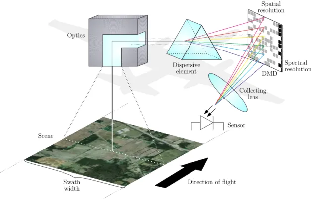
Zun¨achst werden niedrigdimensionale Methoden f¨ur die Klassifikation mit Anwendung in der hyperspektralen Bildgebung vorgestellt. In der Fernerkundung stellt die hyper-spektrale Bildgebung ein effizientes Mittel zur Analyse großer Areale bereit. Insbeson-dere k¨onnen mit den aufgezeichneten Daten verschiedene Materialien einfach unter-schieden werden, da jedes Element des aufgezeichneten Bildes das Spektrum des sicht-baren sowie des infraroten Lichts darstellt. F¨ur die Klassifikation wird ein Ansatz zur Auswahl der Merkmale und zur effizienten Aufzeichnung der Daten vorgestellt. Das Ziel beider Methoden besteht darin, die Menge der Daten, die w¨ahrend der Klassifikation ausgewertet werden muss, zu reduzieren, wobei hohe Klassifikationsgenauigkeiten er-halten werden sollen. Im ersten Ansatz wird einecluster-basierte Methode zur Auswahl der B¨ander des hyperspektralen Bildes vorgestellt, welche als Merkmale f¨ur die Klassi-fikation betrachtet werden k¨onnen. Da das Entfernen aufw¨andig aufgezeichneter Daten zu einer ineffizienten Nutzung der Ressourcen f¨uhrt, wird weiterhin ein Ansatz zur Aufzeichnung basierend auf Compressive Sensing vorgestellt. Der Kerngedanke dieser Methode besteht darin, die Daten in einer niedrigdimensionalen Darstellung aufzuze-ichnen. F¨ur die Klassifikation k¨onnen diese Daten als eingebettet in einem Merkmal-sraum betrachtet werden. Da wir direkt an einer Klassifikation interessiert sind, ist eine aufwendige Rekonstruktion der Daten nicht notwendig und kann vermieden werden. Weiterhin wird ein merkmalsbasiertes Verfahren zum Erlernen von Strukturen in den Spektren vorgeschlagen, welches die in den hyperspektralen Bildern vorkom-menden Materialien extrahiert. Hyperspektrale Bilder weisen oft eine geringe r¨aumliche Aufl¨osung auf, so dass die Elemente des Bildes große Areale darstellen, oft im Bereich von 2 m2 bis 400 m2. Viele Algorithmen, die u.a. zur Klassifikation verwendet werden, nehmen jedoch an, dass jedes Bildelement nur ein einzelnes Material darstellt. Folglich
IV
ist das Erlernen der Struktur eine wichtige Aufgabe in der hyperspektralen Bildgebung. Dies wird auch als spektrales unmixing bezeichnet. Hierf¨ur wird eine Bayessche nicht-parametrische Formulierung des Problems vorgeschlagen. Ein wichtiger Vorteil dieses Modells im Vergleich zu bestehenden Methoden ist, dass die Anzahl der Materialien aus den Daten inferiert werden kann und somit nicht als bekannt vorrausgesetzt wird. Die vorgeschlagene Formulierung resultiert in einem Bayesschen nichtparametrischen unmixing Algorithmus, der in der Lage ist, die Anzahl der Merkmale, die Merkmale selbst, sowie deren Koeffizienten gemeinsam zu lernen.
Zuletzt wird ein Modell f¨ur die Entscheidungsfindung vorgeschlagen, das auf Merkmals-darstellungen der Beobachtungen basiert. Insbesondere wird das Problem des Lernens aus Beobachtungen mit dem Ziel betrachtet, ein Verhalten aus den Beobachtungen eines erfahrenen Agenten zu lernen. Ein bedeutender Unterschied zu bestehenden Verfahren liegt in der Annahme, dass der Agent seine Entscheidungen basierend auf Merkmalen der Beobachtungen trifft, wobei jedes Merkmal eine bestimmte Entschei-dung impliziert. Das Erlernen der Merkmale und deren Verhaltensregeln erm¨oglicht es Schl¨usse ¨uber das beobachtete Verhalten zu ziehen. Weiterhin k¨onnen Aktionen f¨ur neue Situationen vorhergesagt werden, aus denen Verhaltensregeln f¨ur andere Agen-ten abgeleitet werden k¨onnen. Um die M¨oglichkeiAgen-ten des Modells anhand eines realen Problems aufzuzeigen, wird mithilfe des entwickelten Algorithmus das Verhalten eines Fahrers analysiert, welches eine typische Aufgabe in intelligenten Fahrerassistenzsyste-men ist.
Die Algorithmen, die auf den vorgeschlagenen Modellen basieren, werden mithilfe simulierter Daten zur ¨Uberpr¨ufung der Konzepte ausgewertet. Weiterhin werden alle Methoden auf reale Daten angewandt, um die Leistungsf¨ahigkeit der entwickelten Ans¨atze zu demonstrieren.
V
Abstract
Many signal processing and machine learning algorithms perform poorly when applied to high-dimensional data, as is known by the phenomenon of the curse of dimension-ality. Learning low-dimensional representations aims at reducing the dimensionality of the observation space while maintaining the characteristics of the data. Further, low-dimensional representations can help to reveal latent structures, allowing for deeper insights into the observations. For these reasons, models are proposed that allow to learn low-dimensional representations of the observations, providing means for the anal-ysis of the observed data. In particular, approaches for efficient data acquisition and classification and for the inference of the structure of the observed data are presented. First, low-dimensional methods for classification are proposed with application to hy-perspectral imaging. In remote sensing, hyhy-perspectral imaging provides an efficient means for the analysis of vast areas. As each element of the captured image represents the spectrum of the visible and infra-red light, the acquired data allows for effective discrimination between different materials. For classification, a feature selection ap-proach as well as a sparse acquisition scheme are presented. The goal of both methods is to reduce the amount of data that needs to be evaluated during classification, while maintaining high classification accuracies. In the first approach, a clustering-based method for selecting the bands of a hyperspectral image, which can be considered as features for classification, is proposed. However, removing costly acquired data during feature selection is clearly resource-inefficient. For this reason, further a sparse acqui-sition approach based on the Compressive Sensing framework is proposed. The key idea of this approach is to capture the data in a low-dimensional representation, which is interpreted as being embedded in a feature space for the classification problem. As we are interested in the classification result directly, costly reconstruction of the data is not required and can be avoided.
Second, a feature-based approach to learn the structure of the spectra is proposed, revealing the materials present in a hyperspectral image. Hyperspectral images often suffer from low spatial resolutions such that each element of an image represents a large area, often in the range from 2 m2 to 400 m2. However, many algorithms, such as for classification, assume that each element of the image represents a single material only. Thus, learning the structure is an important task in the analysis of hyperspectral images, which is also known as spectral unmixing. For this, a Bayesian nonparametric formulation of the problem is proposed. A significant advantage of this model, in comparison to existing approaches, is that the number of materials is inferred from the data and, hence, is not required to be known a priori. The proposed formulation
VI
results in a Bayesian nonparametric unmixing algorithm which enables to learn the number of latent features, the actual features, and their coefficients jointly.
Third, a model for decision-making based on a feature representation of the observa-tions is proposed. In particular, the problem of learning from observaobserva-tions is considered, in which we aim at learning a behavior from observations which are provided by an experienced agent. A key difference to existing approaches consists in the assumption that the agent makes its decision based on latent features of the observations, where each feature indicates a certain action. Learning the features and their policies enables to reason about the observed behavior. Further, actions for new situations can be predicted, from which a policy can be derived for other agents. Using the developed algorithm, a driver’s behavior is analyzed, which is a typical task in advanced driver assistance systems, in order to show the performance of the model in a real-world problem.
The algorithms based on the proposed models are evaluated on simulated data to proof the concepts. Further, all methods are applied to real data, demonstrating the high performance of the developed approaches.
VII
Contents
1 Introduction and Motivation 1
1.1 State of the Art . . . 2
1.2 Contributions . . . 5
1.3 Publications . . . 6
1.4 Organization of the Thesis . . . 7
2 Machine and Feature Learning Fundamentals 9 2.1 Computational Learning Theory . . . 9
2.1.1 Statistical Learning Theory . . . 9
2.1.2 Bayesian Inference . . . 11
2.1.3 Curse of Dimensionality . . . 12
2.2 Approximate Inference Techniques . . . 13
2.2.1 Metropolis and Metropolis-Hastings Sampling . . . 13
2.2.2 Gibbs Sampling in a Directed Graphical Model . . . 14
2.2.3 Parallel Tempering . . . 16
2.3 Feature Learning and Low-Dimensional Representations . . . 17
2.3.1 Feature Models . . . 17
2.3.2 Low-Dimensional Data Acquisition Using Compressive Sensing . 18 2.3.3 Bayesian Feature Learning . . . 19
2.4 Clustering and Classification . . . 24
2.4.1 Spectral Clustering . . . 24
2.4.2 k-Nearest Neighbor . . . 26
2.4.3 Support Vector Machine . . . 27
3 Feature Learning for Classification in Hyperspectral Imaging 33 3.1 Motivation and Introduction . . . 33
3.2 Hyperspectral Image Data Sets . . . 35
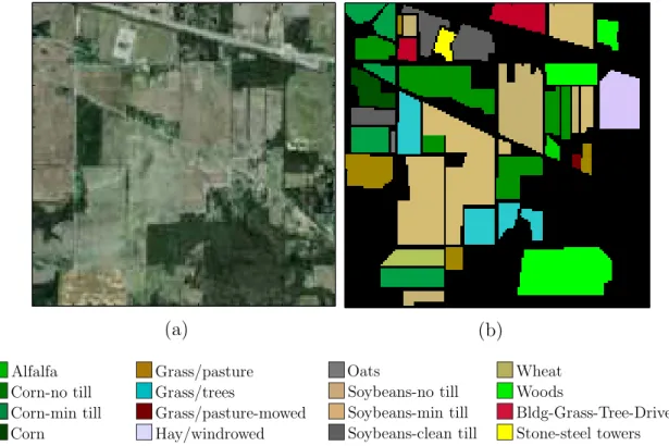
3.2.1 Indiana’s Indian Pines (IP) . . . 35
3.2.2 University of Pavia (UP) and Center of Pavia (CP) . . . 36
3.2.3 Acknowledgment . . . 38
3.3 Band Selection by Means of Spectral Clustering . . . 38
3.3.1 Cluster Formation . . . 38
3.3.2 Representative Selection . . . 39
3.3.3 Classification . . . 40
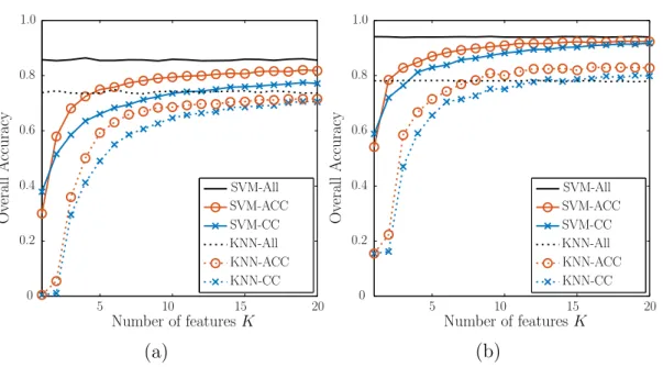
3.3.4 Results . . . 41
3.4 Classification in the Compressive Domain . . . 44
VIII Contents
3.4.2 System Design . . . 46
3.4.3 Optimization of the Acquisition Process . . . 47
3.4.4 Results . . . 51
3.5 Conclusions . . . 53
4 Hyperspectral Unmixing via Bayesian Nonparametric Feature Learn-ing 55 4.1 Motivation and Introduction . . . 55
4.2 State of the Art . . . 56
4.3 Contribution . . . 57
4.4 Bayesian Nonparametric Unmixing Model . . . 58
4.4.1 Observation Likelihood . . . 59
4.4.2 Prior for the Noise Variance . . . 59
4.4.3 Prior for the Abundances . . . 60
4.4.4 Prior for the Endmember Weights and Activations . . . 60
4.4.5 Joint Posterior Distribution . . . 61
4.5 Inference . . . 61
4.5.1 Sampling the Noise Variance . . . 61
4.5.2 Sampling the Abundances . . . 62
4.5.3 Sampling the Endmember Weights . . . 62
4.5.4 Sampling the Endmember Activations . . . 63
4.5.5 Sampling Procedure . . . 65
4.6 Experimental Results . . . 66
4.6.1 Simulations . . . 69
4.6.2 Real Data . . . 76
4.7 Discussion and Outlook . . . 80
4.8 Conclusion . . . 82
5 Bayesian Feature-Based Learning From Demonstrations 83 5.1 Motivation and Introduction . . . 83
5.2 Contributions . . . 84
5.3 Problem Formulation . . . 85
5.4 State of the Art . . . 86
5.4.1 Reinforcement Learning . . . 86
5.4.2 Inverse Reinforcement Learning . . . 87
5.4.3 Imitation Learning . . . 88
5.5 Choice of the Model . . . 88
5.5.1 Feature Model for Learning From Demonstrations . . . 88
5.5.2 Transition Model . . . 89
Contents IX
5.5.4 Alternative Feature-Based Models . . . 90
5.6 Bayesian Nonparametric Model for Feature Learning . . . 92
5.6.1 Observation Likelihood and Noise Variance . . . 92
5.6.2 Prior for the Feature Weights and Activations . . . 92
5.6.3 Prior for the Substates . . . 93
5.6.4 Mixture of Policies and Action Likelihood . . . 94
5.6.5 Joint Posterior Distribution . . . 95
5.7 Inference . . . 95
5.7.1 Conditional Distributions . . . 96
5.7.2 Sampling Algorithm . . . 99
5.7.3 Prediction of Actions . . . 100
5.8 Experimental Results . . . 101
5.8.1 Estimation of the Features . . . 102
5.8.2 Prediction of Actions . . . 102
5.8.3 Estimation of the Number of Features . . . 104
5.9 Real Data Experiments . . . 106
5.9.1 Scene 11 - Traffic Jam . . . 108
5.9.2 Scene 20 - Lane Change . . . 113
5.10 Discussion . . . 114
5.11 Conclusion . . . 116
6 Conclusions and Outlook 117 6.1 Summary and Conclusions . . . 117
6.1.1 Feature Learning for Classification in Hyperspectral Imaging . . 117
6.1.2 Hyperspectral Unmixing via Bayesian Nonparametric Feature Learning . . . 118
6.1.3 Feature-Based Decision-making . . . 119
6.2 Outlook . . . 119
6.2.1 Low-Dimensional Representations for Classification in Hyper-spectral Imaging . . . 119
6.2.2 Features for the Analysis of Hyperspectral Images . . . 120
6.2.3 Features for the Analysis and Prediction in Decision-Making Problems . . . 121
A Derivations for Compressive Classification 123 B Derivations for Bayesian Nonparametric Feature Learning 125 B.1 Conditionals for the Feature Weights . . . 125
B.1.1 Using the Distance Prior . . . 126
X Contents
B.1.3 Using a Gaussian Prior . . . 128 B.2 Conditional for the Noise Variance . . . 129 B.3 Sparsity-Promoting Prior on the Feature Coefficients . . . 129
List of Acronyms 131
List of Symbols 135
Bibliography 145
1
Chapter 1
Introduction and Motivation
Processing large amounts of data has become increasingly important in the recent past and is required in a wide range of applications. Prominent examples can be found in remote sensing [1], social networks [2], recommender systems [3], and intelli-gent robotics [4]. These applications usually incorporate regression, classification, and decision-making where many data samples (observations) need to be evaluated such that conclusions can be drawn. A key problem of many algorithms used for data anal-ysis is their poor performance in case of high-dimensional input data – a phenomenon which is widely known as the curse of dimensionality [5].
Often, a feature representation is chosen to reduce the dimensionality of the data and to overcome the problems induced by the curse of dimensionality. For this purpose, it is typically assumed that the relevant information contained in the observations is embedded in a subspace. Thus, features enable for a problem-specific representation of the data in which important characteristics are retained, while irrelevant information is reduced. A crucial question for many data analysis methods, e.g., for classification and regression, is the choice of features. Depending on the feature representation, the analysis may succeed or, in the worst case, fail completely. In many applications, features are handcrafted, requiring an expert of the respective domain to design them. Often, the data that shall be analyzed is complex and the design of the features is carried out in a trial-and-error approach. Thus, it is desirable to learn features from the observed data directly [6].
Besides reducing the size of the data to increase the efficiency of the post-processing steps, such as classification, low-dimensional representations can also be used to learn the structure of the data. In many applications, features have a specific meaning and can, therefore, be interpreted by experts. If we are able to learn the features present in the data in compliance with our prior assumptions, we can obtain a deeper understanding of the observations. An example can be found in hyperspectral imaging. Here, the features of the pixels can be considered as the spectral signatures of the pure materials present in the captured scene [7, 8].
In this thesis, we address the problem of learning low-dimensional representations from observed data. We refer to this problem as Feature Learning (FL). As the transforma-tion into the low-dimensional space as well as the projectransforma-tions of the observatransforma-tions are
2 Chapter 1: Introduction and Motivation
unknown, this problem can be considered as a Blind Source Separation (BSS) prob-lem. Many methods have been developed in the past to solve BSS problems, famous examples are Principal Component Analysis (PCA) [9, 10], Independent Component Analysis (ICA) [11], and Non-negative Matrix Factorization (NMF) [12]. However, most methods make specific assumptions about the observed data and their structure that may not hold for the problem at hand. Further, many algorithms assume the number of latent features to be known, which is rarely the case in practice.
In this thesis, we propose different feature selection and learning techniques that aim at improving post-processing steps and allow for an accurate analysis of the data. In particular, we investigate statistical methods for low-dimensional data acquisition and Bayesian models to identify the latent structure of the data. For the latter, we pro-vide means to infer the number of features by making use of Bayesian Nonparametric techniques [13]. At this point we would like to clarify, though FL is generally not restricted to learning low-dimensional representations, e.g., kernel methods often op-erate on a feature space larger than the space of observations, we understand FL as learning low-dimensional representations of the observations. Throughout the thesis, we thus use the terms low-dimensional representations and features representations interchangeably.
1.1
State of the Art
Various feature selection and learning methods have been proposed in the past. An exhaustive overview about feature learning would fill a book on its own. Thus, in this section, we concentrate on important work that is relevant for this thesis.
While in feature selection, one assumes that a set of features is available, where the task is to estimate the presence of the features in the observations, FL aims at estimating the features itself. As explained in [14], one can distinguish between two categories of FL: (i) extrinsic and (ii) intrinsic methods. Extrinsic methods are independent of the post-processing algorithm and, therefore, can be used with many methods. For example, PCA [9, 10], ICA [11], and NMF [12] belong to this category. Due to their nature, application-specific constraints can often not be incorporated and assumptions are being made that may not hold for the problem at hand. In contrast, intrinsic methods are integrated in the post-processing algorithm, and thus need to be designed or at least be adapted to the algorithm and application. A general framework for this purpose is Bayesian Feature Learning (BFL) [15–17] which is formulated as a generative model and, thus, can be adapted and extended to the problem.
1.1 State of the Art 3
In some research communities, features are also referred to as entries of a codebook or dictionary. One of the most prominent and successful approaches to FL is sparse coding [18], where a linear latent feature model is derived with sparse feature coefficients. Further, a dictionary is learned by iterating between the estimation of the coefficients and the dictionary. Sparse coding has shown good results in computer vision [19–21] and audio applications [22]. There have been several extensions to this work. For example, in [23], Local Coordinate Coding (LLC) is presented that exploits local linear models, with the goal of fast learning large dictionaries. A high dimensional dictionary is learned by k-means clustering which is used to transform the observations into a sparse representation. Locality is exploited by assuming a linear relation between the observations and the basis spanned by the k-nearest neighbors.
In the recent past, spike and slab models have demonstrated excellent performance for feature learning. Spike and slab models assume that a variable is composed of the latent spike, a binary variable, and the latent slab, a variable of a domain defined by the application [24, 25]. In feature learning, the slab corresponds to the weight of an element of a feature vector. The spike can be understood as a feature activation that activates the corresponding weight depending on the observed data samples [26]. The concept of sparse coding has been combined with the spike and slab model into a deep architecture in [27], showing high accuracies in image classification as well as transfer learning.
FL has changed significantly since the development of deep architectures in the con-text of the Deep Learning (DL) framework. The idea of stacking multiple processing layers to learn features and perform classification, e.g., using several hidden layers in a neural network, posed huge challenges for training in the past. Naive gradient-based ap-proaches (such as the backpropagation algorithm [28,29]) using random initialization of the network weights usually fail at learning networks with several hidden layers. There are two potential explanations for this. First, the noise in the gradient increases with each layer, providing insufficient information about the parameters to be learned [30]. Second, due to the high flexibility of the model, overfitting is likely to occur and ef-fective regularization is needed [30]. In 2006, a new method for training multi-layered networks has been proposed, referred to as pre-training, which initializes the layers by means of unsupervised training [6, 30–32]. Since pre-training does not require class information, which is usually expensive to obtain, the network can easily be trained on huge amounts of data. Given a good initialization of the network layers, a refinement of the parameters is conducted using conventional supervised learning techniques. As the hidden layers can be understood as feature hierarchies [32–34], DL provides means to learn nonlinear features from observed data, with low-level features in the bottom
4 Chapter 1: Introduction and Motivation
layers and more abstract, high-level features in the top layers. DL has shown out-standing results in many applications, e.g., in image processing [35] and especially in automated speech recognition [36–38].
Some FL approaches have been extended for the use in time-sequential data, e.g., for feature analysis in videos. Slow Feature Analysis (SFA), which can be considered as an extension of ICA, assumes that the relevant information of a time varying signal is con-tained in a slowly varying latent signal [39]. This latent signal can then be considered as the features of the observed signal. In [40], SFA has been extended to decision-making problems, referred to as Contingent Feature Analysis. In this approach, features are sought for that explain the high variance of the temporal derivatives of the observed states, if the agent performs an action. A different approach based on DL has been taken in [41], where the independent subspace analysis algorithm [42] has been ex-tended such that features are directly learned from video material, resulting in highly accurate action recognition. Recent research has demonstrated the performance of DL also in decision-making problems [43, 44].
Especially in image formation, capturing the data at Nyquist rate and then transform-ing it into a low-dimensional representation is inefficient, as costly acquired data is literally thrown away. A framework that allows for the acquisition of data below the Nyquist rate is given by Compressive Sensing (CS) [45, 46]. In CS, one assumes that the data that shall be captured can be sparsely represented in a certain domain. Un-der certain conditions, the data can be perfectly reconstructed from the few captured samples. CS can be also understood as capturing a low-dimensional representation directly at the sensing level. However, finding suitable sparse transformation and mea-surement matrices, which can be considered as a linear feature transform, is generally challenging. While the literature on CS is exhaustive, only few work is concerned with learning the dictionary for CS, e.g., [47, 48].
The state of the art of FL is currently dominated by DL. Though these models show excellent results, they possess significant drawbacks. First, it is not easy to incorporate prior assumptions in deep architectures. If FL is used for data analysis with the aim to learn about the structure of the observed data, DL does not present a suitable approach as the learned representations are often difficult to interpret. Second, training is highly challenging since these architectures are able to represent highly complex nonlinear models. Thus, there is no guarantee that (globally) optimal parameters are learned with respect to classification accuracy. Further, despite the compactness of these models, a huge number of parameters has to be learned, requiring large amounts of data and vast computation facilities. Though costs for computation power has significantly decreased with the availability of massively parallel computer architectures such as
1.2 Contributions 5
graphics cards and clusters, computation time is still an issue for practical data analysis. More important than that, for many problems we do not have access to large amounts of observations for training the model. Instead, we often have an intuition about the characteristics of the data, which can be exploited to constrain the model. By this, the flexibility of the model can be reduced and, hence, the number of parameters that need to be learned, making inference more efficient in the sense of data and computation efficiency.
1.2
Contributions
We propose different feature selection and learning techniques with applications to hy-perspectral imaging and decision-making. For hyhy-perspectral imaging applications, we consider a feature selection scheme for classification and a low-dimensional acquisition method for direct classification of the observed data. Moreover, a Bayesian approach for unmixing hyperspectral images based on BFL is proposed. Finally, we extend the BFL framework to learn feature representations in decision-making problems.
In summary, the contributions of this thesis are as follows:
• Band selection for hyperspectral imaging
We provide a simple yet effective algorithm that selects relevant bands of a hy-perspectral image which serve as features for classification. Operating in the subspace of the observed data, we provide means to estimate the number of relevant bands.
• Classification based on sparsely acquired hyperspectral image data
Capturing hundreds of bands and removing many of them during band selection is resource-inefficient. Thus, we present an acquisition scheme that directly captures the relevant information of the scene. The proposed framework is based on CS but skips the costly reconstruction of the data. Instead, the compressively sensed data is considered as a low-dimensional representation and is directly classified. To improve the classification accuracy, we show how the sensing and transformation matrices can be learned from training data.
• Inferring the latent number of endmembers, the endmembers, and their fractional abundances in hyperspectral images
Based on BFL, we consider an algorithm that decomposes the elements of a hyperspectral image into its endmembers and their fractional abundances. As the
6 Chapter 1: Introduction and Motivation
number of latent endmembers is rarely known in practice, we present a Bayesian nonparametric extension that is also able to estimate the number of endmembers.
• Feature-based decision-making
We adapt and extend BFL to a Bayesian nonparametric formulation for behavior analysis in the context of decision-making. We assume that the observed agent makes its decision based on latent features of the observed state. These features can then be interpreted as causes that influenced the agent to make the observed decision. Our goal is to learn this representation, which provides insights into the reasoning of the agent. Additionally, the proposed model allows for a compact state representation that can be used for efficient prediction of actions for new observations.
1.3
Publications
The following publications have been produced during this doctoral project.
Internationally Refereed Journal Articles
• J. Hahn and A. M. Zoubir, “Bayesian Nonparametric Feature and Policy Learning for Decision Making”, submitted toPattern Recognit, 2016
• J. Hahn and A. M. Zoubir, “Bayesian Nonparametric Unmixing of Hyperspectral Images”, submitted to IEEE Trans Geosci Remote Sens, 2016
• C. Debes, A. Merentitis, R. Heremans, J. Hahn, N. Frangiadakis, T. van Kasteren, W. Liao, R. Bellens, A. Pizurica, S. Gautama, W. Philips, S. Prasad, Q. Du, and F. Pacifici, “Hyperspectral and LiDAR Data Fusion: Outcome of the 2013 GRSS Data Fusion Contest” IEEE J Sel Topics Appl Earth Observ, Vol 7, No 6, pp. 2405-2418, Mar. 2014
• J. Hahn, C. Debes, M. Leigsnering, and A. M. Zoubir, “Compressive Sensing and Adaptive Direct Sampling in Hyperspectral Imaging”, Digit Signal Process, Vol 26, No 3, pp 113-126, Mar. 2014
1.4 Organization of the Thesis 7
Internationally Refereed Conference Papers
• J. Hahn and A. M. Zoubir, “Risk-Sensitive Decision Making via Constrained Ex-pected Returns”, Proc. IEEE Int Conf Acoust Speech Signal Process. (ICASSP) 2016 in Shanghai, China, pp. 2569-2573, Mar. 2016
• S. Shukanov, A. Merentitis, C. Debes, J. Hahn, and A. M. Zoubir, “Bootstrap-Based SVM Aggregation for Class Imbalance Problems”, Proc. Eur Signal Pro-cess Conf (EUSIPCO) 2015 in Nice, France, pp. 165-169, Sept. 2015
• J. Hahn and A. M. Zoubir, “Inverse Reinforcement Learning Using Expectation Maximization in Mixture Models”, Proc. IEEE Int Conf Acoust Speech Signal Process (ICASSP) 2015 in Brisbane, Australia, pp. 3721-3725, Apr. 2015
• J. Hahn, S. Rosenkranz, and A. M. Zoubir, “Adaptive Compressed Classification for Hyperspectral Imagery”, Proc. IEEE Int Conf Acoust Speech Signal Process (ICASSP) 2014 in Florence, Italy, pp. 1020-1024, May 2014
• V. Kumar, J. Hahn, and A. M. Zoubir, “Band Selection for Hyperspectral Im-ages Based on Self-Tuning Spectral Clustering”, Proc. Eur Signal Process Conf (EUSIPCO) 2013 in Marrakech, Morocco, pp. 1-5, Sept. 2013
1.4
Organization of the Thesis
The thesis is structured as follows. In Chapter 2, an introduction to machine learn-ing theory is given. Further, basic feature learnlearn-ing and classification approaches are presented that are used throughout the thesis.
In Chapter 3, we first introduce a band selection algorithm for classification. Since the bands serve as features for the classifier, this approach can be considered as a feature selection algorithm tailored to hyperspectral imaging. In the same chapter, we present an alternative approach that aims at capturing image data in a low-dimensional representation directly by means of the CS framework. Since we are interested in the classification of the image instead of the actual hyperspectral image, we skip the costly reconstruction step and consider the captured data as a low-dimensional feature representation that is directly classified. The proposed method is adaptive in the sense that the measurement and basis matrices are learned from training data.
In Chapter 4, we present a Bayesian nonparametric framework for hyperspectral un-mixing. This framework is able to jointly infer the endmembers present in the scene,
8 Chapter 1: Introduction and Motivation
their fractional abundances and, in contrast to many existing approaches, the number of the endmembers. The proposed algorithm is evaluated with simulated as well as real data.
In Chapter 5, the Bayesian feature learning framework is extended and applied to a decision-making problem. We assume that the agent, whose states and actions can be observed, acts upon latent features of the observations. Thus, each feature indicates a certain policy, leading to a mixture of policies the agent follows. In particular, we are interested in learning the features and their policies, as they provide a deeper understanding of the observed behavior as well as a compact representation of the states, allowing for efficient prediction of actions for new, previously unobserved states. Finally, in Chapter 6, conclusions are drawn and an outlook for future perspectives is given.
9
Chapter 2
Machine and Feature Learning
Fundamentals
In this chapter, we give an introduction to computational learning theory. Based on the presented concepts, inference techniques and methods for dimensionality reduction and classification are explained which are used throughout this thesis.
2.1
Computational Learning Theory
Computational learning theory provides means to understand and to model learning problems, and enables performance analysis of developed algorithms. There exist many different philosophies in the field of learning theory, though many theories are based on similar ideas and possess common assumptions. In this thesis, we rely on statistical learning theory [49] and Bayesian inference to model the given learning problems.
2.1.1
Statistical Learning Theory
Statistical learning theory describes the act of learning from experience to draw con-clusions about future observations, referred to as predictions [49, 50]. Essentially, this can be described as learning a mapping, fθ : z 7→y, where z ∈ ZD×1 is the observed
data sample of dimension D and θ ∈ Θ describes the parameters of the function fθ.
The parameters are learned from previously observed data D and are used to predict the label y ∈ Y. If Y denotes a finite set, we refer to problem as classification, while in contrast, if Y is an infinite set, we refer to the problem as regression. This scheme is illustrated in Fig. 2.1.
For learning θ, a loss function, L, is defined, which penalizes incorrect predictions.
During learning, the expected risk shall be minimized, which is the expectation of the loss function, ERisk(f) = Z Z Z YL (fθ(z), y)p(z, y) dzdy, (2.1)
10 Chapter 2: Machine and Feature Learning Fundamentals
D
z
f
θ(
z
)
y
Figure 2.1. Learning refers to estimating the parameters, θ, of function fθ from
pre-viously observed data D. A label, y, for observation data, z, can then be predicted based on θ.
where p(z, y) denotes the joint distribution of the observations, z, and their labels, y. Since this distribution is generally unknown, it is approximated by the samples con-tained in the training setDT ={(zT,1, yT,1), . . . ,(zT,NT, yT,NT)}, yielding the empirical
risk, EEmp(f) = 1 NT NT X n=1 L(fθ(zT,n), yT,n). (2.2)
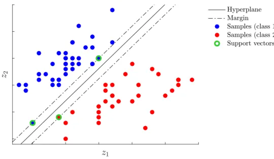
The empirical risk in Eq. (2.2) converges to the true risk in Eq. (2.1) for an infinite number of training samples,NT → ∞. In practice, however, the size of the training set is often limited to a few samples, such that the empirical risk only poorly approximates the true risk. Then, minimizing the empirical risk does not guarantee to provide good estimates of the parameters. This is related tooverfitting, which describes the problem that the parameters θ are well adapted to the training set, but do not generalize well to unobserved data. Structural risk minimization aims at solving this problem by finding a “tradeoff between the quality of the approximation and the complexity of the approximating function” [49] and has resulted, e.g., in the development of the Support Vector Machine (SVM) [51]. The SVM is explained in Section 2.4.3.
Learning problems where predictions are part of the training data set are referred to as supervised learning tasks and are well understood in the framework of statistical learn-ing theory. If the trainlearn-ing data set, DT, only consists of the observationsz1, . . . ,zNT,
we refer to the problem as an unsupervised learning task. There are other types of learning problems, such as online or reinforcement learning, that are not considered in this thesis. Though the observations in the decision-making problem in Chapter 5 underlie a Markov Decision Process (MDP), the problem we consider can be reduced to a supervised one. For completeness, we will briefly introduce concepts and models for decision-making in Chapter 5.
2.1 Computational Learning Theory 11
2.1.2
Bayesian Inference
A different, yet similar paradigm to the statistical learning framework is statistical in-ference [52,53]. Statistical inin-ference provides means for understanding both supervised and unsupervised problems by building models that aim at explaining the observed data.
In this thesis, we mainly rely on Bayesian inference, a subarea of statistical inference, that we consider in particular in Chapters 4 and 5. Bayesian inference is a universal tool which provides means for modeling various problems and inferring solutions. Prior assumptions and constraints can be easily incorporated, making it interesting to be used in feature learning [17]. In the following, we briefly introduce the fundamentals of Bayesian inference.
A key assumption of Bayesian inference is that observed data cannot be explained by fixed parameters. Instead, the parameters are considered as variables, in the following denoted byθ. Placing a prior distribution over the variables,p(θ), the goal is to derive the posterior distribution,p(θ| D), over the possible parameters, providing information about how probable a certain parameter is given the set of observations, D. Using Bayes’ theorem, we can express the posterior in terms of the likelihood, p(D |θ), and the prior, p(θ), p(θ| D) | {z } posterior = p(D |θ)p(θ) p(D) ∝p|(D |{zθ)} likelihood p(θ) |{z} prior . (2.3)
To find an expression for the posterior p(θ| D), the factorization in Eq. (2.3) is ex-ploited. Prior knowledge or general assumptions on the parameters can be incorporated into the prior. The normalization, referred to as evidence, given by p(D), is usually not considered as it is independent of the parameters. As the posterior is often not analytically tractable, one has to resort to approximate inference techniques. This is detailed in Section 2.2.
For prediction, Bayesian inference averages over all possible explanations represented by θ. Given the training data, D, and an observation, z?, we want to infer the
corre-sponding value y?, which is achieved by means of the posterior predictive distribution:
p(y? |z?, D) = Z Θ p(y?,θ |z?, D) dθ = Z Θ p(y?|θ,z?)p(θ|z?,D) dθ.
12 Chapter 2: Machine and Feature Learning Fundamentals
D = 1 D = 2 D = 3
Figure 2.2. Illustration of the exponential growth of the volume of the space with increasing dimension D. As the number of samples (red dots) is kept constant the coverage of the space becomes highly sparse.
Here, we assume that the parameters,θ, contain all relevant information such that y?
is independent of D given θ.
In general, θ depends on the training data,D, and the new observation,z?. Thus, the
posterior in Eq. (2.3) has to be estimated for every new observation. However, if the training samples sufficiently characterize θ, the influence of z? onθ is relatively small
such that the dependency on the new observations can be ignored, reducing prediction time significantly.
2.1.3
Curse of Dimensionality
Many machine learning and statistical inference techniques show poor performance with increasing dimensionality of the data. Thecurse of dimensionality, also known as Hughes effect [5], explains the fact why the required number of training samples grows exponentially with the dimensionality of the data to counteract this phenomenon [54]. As illustrated in Fig. 2.2, with growing dimensionality, the observation space increases exponentially, leading to a sparse coverage by training samples.
Many signal processing and machine learning algorithms suffer from this fact. The training samples are hardly able to represent the distribution of the data, which makes learning the underlying structure difficult and results in a poor prediction performance. This effect can be easily explained by means of the statistical learning framework, as the empirical risk, Eq. (2.2), becomes a poor approximation of the true risk, Eq. (2.1). For this reason, it is often desirable to find a low-dimensional representation of the data, which can be understood as a feature representation. Note that, however, reducing the
2.2 Approximate Inference Techniques 13
dimensionality to a minimum does not always result in a better performance. A good counterexample can be found in classification, where a high-dimensional representation often helps to separate the classes.
2.2
Approximate Inference Techniques
In many applications, the posterior, which is sought for in Bayesian inference, is ana-lytically intractable. We encounter this problem in the hyperspectral unmixing model and the decision-making problem in Chapters 4 and 5, respectively.
For this reason, techniques for approximating the posterior are required. On the one hand, we can try to express the posterior by a simpler distribution that allows for an an-alytic solution as in variational methods, c.f. [55]. On the other hand, we can represent the posterior by samples, known as Monte Carlo techniques, c.f. [56]. Sampling based approaches have the advantage that they are able to perfectly represent the distribu-tion if, in the limit, an infinite number of samples is given. The main drawback is that, usually, sampling is more time consuming compared with variational techniques [53]. Though variational approaches are often significantly faster, we only consider sampling based approaches as the approximations in the variational framework can introduce a bias. Well-known sampling algorithms are the Metropolis-Hastings algorithm and the Gibbs sampler, which are introduced in the following sections.
2.2.1
Metropolis and Metropolis-Hastings Sampling
Consider the problem of generating samples of the random variable θ∈Θ, where the probability density function (pdf) of θ, referred to as target pdf, can be written as
p(θ) = 1
Zθ
˜
p(θ),
with ˜p(θ) denoting a factor dependent on θ. In general, sampling from p(θ) can be challenging, especially if the normalization constant Zθ is unknown. Metropolis et
al. [57] proposed an iterative method for sampling from p(θ) using a proposal distri-bution, q(θ(t)|θ(t−1)), one can easily sample from, with t, t = 1, . . . , NS, denoting the
tth sample. The proposal θ(t) generally depends on the previously generated sample θ(t−1), where the first sample can be initialized arbitrarily. Hence, this sampler forms a Markov chain.
14 Chapter 2: Machine and Feature Learning Fundamentals
In each iteration, the tth proposed sample θ(t) is accepted with probability PM = min(rM,1), with acceptance ratio
rM= ˜
p(θ(t)) ˜
p(θ(t−1)).
If the sample is rejected, the previous sample is kept, i.e., θ(t) ← θ(t−1). Note that several iterations, known as the burn-in phase, are required until samples from the target distribution are drawn.
A key limitation of this algorithm is the assumption that the proposal distribution is symmetric, i.e., q(θ(t)|θ(t−1)) = q(θ(t−1)|θ(t)). The Metropolis-Hastings (MH) algo-rithm [58] generalizes the Metropolis algoalgo-rithm by incorporating the probabilities of the proposals into the modified acceptance ratio, rMH, with
rMH = ˜ p(θ(t))q(θ(t−1) |θ(t)) ˜ p(θ(t−1))q(θ(t) |θ(t−1)).
It can easily be seen that if the proposal distribution is symmetric, the MH algorithm is equal to the Metropolis algorithm. Both algorithms perform a random walk and the samplesθ(t), t = 1, . . . , NS, are distributed according to the target pdf for NS→ ∞. The samples generated by Metropolis sampling are usually highly correlated for mainly two reasons. First, the sampler may repeat samples due to high rejection rates. Second, as the sampler performs a random walk, the differences between the samples might be small, yielding very similar samples. The first problem can be alleviated by choosing a proposal distribution that proposes samples close to previous sample, which, however, increases the second problem. The authors in [59] found that a rejection rate of 0.234 yields a good trade-off. Ideally, we choose a distribution that is very similar to the target pdf. This is the key idea in Gibbs Sampling, which is introduced in the next section.
2.2.2
Gibbs Sampling in a Directed Graphical Model
Sampling high-dimensional variables by means of Metropolis sampling can be highly time consuming due to high rejection rates. We can alleviate this problem by con-sidering each random variable separately, given the other variables. If the conditional of each variable can be derived analytically and be sampled from easily, we may use the conditional as proposal distribution. It can be shown [60] that this results in an acceptance ratio of one such that all samples are accepted. This method is referred
2.2 Approximate Inference Techniques 15
a
b
c
d
e
f
g
h
Figure 2.3. Illustration of a graphical model with variables a–h. As an example, the Markov blanket of d consists of the variables b, c, f, g and e. Observed variables are generally shaded in gray, e.g., c and e.
to as Gibbs Sampling [61] and is frequently used in Bayesian statistics, especially in Bayesian networks. Bayesian networks describe the structure of a multivariate distri-bution in form of the dependencies between the variables and can be represented by a Directed Acyclic Graph (DAG), as opposed to Markov Random Fields (MRFs).
The conditionals, required for Gibbs sampling, are easily derived from a DAG as they are given by theMarkov blanket of the variables [62]. Thus, the conditional of thedth element of the random vector θ can be expressed by
p(θd|θ\d)∝p(θd|pa(θd))
Y
j=ch(θd)
p(θj|pa(θj)),
whereθ\ddenotes all variables except thedth. The operator pa(θ) denotes the parents
of variable θ and ch(θ) its children. An example of a graphical model is depicted in Fig. 2.3, illustrating observed and latent variables and the Markov blanket.
The models we investigate in Chapters 4 and 5 belong to the class of Bayesian networks. For this reason, we consider only Metropolis-Hasting and Gibbs sampling in this chap-ter. However, there exist many other sampling techniques such as slice sampling [63] or Metropolis-Hamilton-Dynamics [64] that provide efficient means for drawing samples from the target distribution.
16 Chapter 2: Machine and Feature Learning Fundamentals
2.2.3
Parallel Tempering
Gibbs sampling is known for getting easily trapped in modes of the joint distribution. In this case, the distribution is not correctly represented by the samples, leading to incorrect inference. This can be detected by running multiple samplers independently in parallel and checking the results for convergence. In order to sample correctly from a multi-modal distribution, Parallel Tempering (PT) [65–67] can be utilized. The key idea, similar as in simulated annealing [61], is to augment the target pdf with another variable, the temperature TPT. Effectively, higher temperatures will smooth out the modes so that other states of the chain, i.e., other realizations of the (modified) distribution, become more probable. Hence, several chains are run in parallel and are exchanged using a Metropolis step.
The algorithm is derived as follows: let the target pdf of the variable θ∈Θ be
p(θ) = 1
Zθ
exp{−U(θ)−V(θ)},
with the two energy terms U(θ), U : Θ → R, and V(θ), V : Θ → R. We augment U(θ) with the temperatureTPT∈ {TPT(1), . . . , TPT(NPT)}whereNPT denotes the number of temperature levels. As an example,U(θ) could describe the energy term of a likelihood, whereasV(θ) could be the energy term of a prior. Thus, augmentingU(θ) only would be equivalent to augmenting the likelihood. For convenience, the temperature levels are ordered, such that
TPT(1) = 1 < TPT(2) < . . . < T(NPT)
PT . The pdf augmented with the ith temperature is given as
p(θ|TPT(i)) = 1
Zθ,T(i) PT
exp{− 1
TPT(i)U(θ)−V(θ)}.
The probability, PPT(ij), of accepting a swap of the ith and the jth chain is
PPT(ij) = min(1, rPT(ij)),
with acceptance ratio r(PTij),
rPT(ij)= p(θj|T (i) PT)p(θi|T (j) PT) p(θi|T (i) PT)p(θj|T (j) PT) = exp{− 1 TPT(j)U(θi)− 1 TPT(i)U(θj)} exp{− 1 TPT(j)U(θj)− 1 TPT(i)U(θi)} = exp{( 1 TPT(j) − 1 TPT(i))(U(θj)−U(θi))}.
2.3 Feature Learning and Low-Dimensional Representations 17
Samples of the target pdf are taken from the first chain withTPT= 1 only. Theoretical results on how to find a suitable number of temperature levels,NPT, and how to set the temperatures can be derived only for simple cases [66]. In practice, one often resorts to setting these parameters in a trial and error approach.
2.3
Feature Learning and Low-Dimensional
Repre-sentations
Feature learning enables the automatic extraction of relevant information from high-dimensional data and to transform it into a low-high-dimensional representation for efficient data analysis.
There are also approaches that transform the observations into a high-dimensional representation, e.g., in kernel machines, c.f. Section 2.4.3. High-dimensional represen-tations are mainly used to improve the separability of the observations as required for classification, for example. However, high dimensional representations are often difficult to interpret and to visualize. For these reasons, and in order to alleviate the curse of dimensionality, in this thesis, we generally understand feature representations as low-dimensional representations of the observed data.
In this section, we revisit methods for acquiring and learning a low-dimensional rep-resentation of the observed data. These approaches present the basis for the tech-niques developed in the following chapters. First, we introduce Compressive Sens-ing (CS) [45, 46], which allows for sparse acquisition of the data. Second, we present a Bayesian approach for learning low-dimensional representations, referred to as Bayesian Feature Learning (BFL). A great advantage of the presented Bayesian approach com-pared with many existing approaches is the possibility to infer the number of features from the data. In other methods, this parameter often has to be set in a trial-and-error approach.
2.3.1
Feature Models
A key difference between CS and BFL is how the features are related to the obser-vations. In the Bayesian formulation, we consider a generative model, i.e., the ob-servations are composed of the features, denoted by FGen, and their low-dimensional
18 Chapter 2: Machine and Feature Learning Fundamentals
representation, sGen,
z=FGensGen. (2.4)
In contrast, CS is related to a projection-based approach, where we interpret the rows of the projection matrix, FDis, as features,
sDis =FDisz, (2.5)
withsDis denoting the projected observations. As this model yields the low-dimensional representation given the features directly, we refer to this approach as discriminative feature learning. In contrast, in the Bayesian model, the representations are part of the generative model. Thus, we refer to the model described in Eq. (2.4) asgenerative feature learning. In the following, we do not differentiate between these models as this will be clear from the context.
2.3.2
Low-Dimensional Data Acquisition Using Compressive
Sensing
In order to capture a signal in a low-dimensional representation directly, the CS frame-work can be used [45, 46]. For this purpose, the signal is required to be sparse in a certain domain. Letz= (z1, . . . , zD)
T
denote a signal of lengthD that can be sparsely represented by means of an orthonormal transformation matrix,Ψ, which describes a
D×D orthonormal basis such that
z =Ψx, (2.6)
where x = (x1, . . . , xD)T denotes the KS-sparse coefficient vector. The KS-sparse
property states that only KS D coefficients are non-zero.
In contrast to conventional sensing following the Nyquist-Shannon sampling theorem [68], not allDsamples of the signalzneed to be captured when using CS. The observed vector s= (s1, . . . , sK)
T
is captured using only K < D measurements, i.e.,
s =Φz+e =ΦΨx+e,
where Φ=
φ1 . . . φKT denotes the K×D measurement matrix and the random vector e describes additive Gaussian noise. For accurate reconstruction, the mea-surement and basis matrices need to be incoherent, which is stated by the Restricted Isometry Property (RIP) [69]. It has been shown that a good choice of Φ is given
2.3 Feature Learning and Low-Dimensional Representations 19
by Gaussian and Bernoulli random matrices [46, 70], which fulfill the RIP with high probability.
For the estimation of z, an under-determined system of equations needs to be solved, which is possible thanks to the sparsity ofx. Consequently, onlyK, withKS ≤K D, measurements are actually required for a highly accurate reconstruction [71]. Thus, the number of samples can be significantly reduced.
The sparsity ofxis exploited during reconstruction by employing a regularization term. Ideally, the l0-norm is considered, resulting however in an infeasible NP-hard problem [72]. In [45, 46], it is shown that minimizing the l1-norm yields a good approximation, i.e., the reconstructed signal ˆxis obtained by
ˆ
x= arg min
x k
xk1 s.t. kΦΨTx−sk2 ≤, (2.7) where is a threshold for the tolerated reconstruction error. Given the estimate ˆx, an estimate of the signal ˆz can be obtained using Eq. (2.6). The optimization problem formulated in Eq. (2.7) can be efficiently solved thanks to the convex shape of the function to be minimized. For this purpose, many algorithms and software packages have been presented, e.g.,l1-magic [73] and SpaRSA [74].
2.3.3
Bayesian Feature Learning
The BFL framework provides a flexible model for inferring the latent structure of the observed data,zn ∈ ZD×1, n= 1, . . . , Nz. For tractability, we focus on a linear feature
model as in [15, 17, 75], which states that each observation is composed of a linear mixture of features, zn= K X k=1 fksn,k+en, n = 1, . . . , Nz, (2.8) with feature coefficient vector sn = (sn,1, . . . , sn,K)T ∈ SK×1 and K feature vectors,
fk ∈ FD×1, k = 1. . . , K. The domain of the observations, Z, the feature coefficients,
S, and the features,F, clearly depend on the application. Thus, the prior distributions for the coefficients and features have to be chosen accordingly.
For example, in Bayesian Non-negative Matrix Factorization (NMF) [17], both the feature coefficients and vectors are assumed to be positive real-valued, which can be expressed by modeling the priors forsn,n= 1, . . . , Nz, andfk,k = 1, . . . , K, as Gamma
20 Chapter 2: Machine and Feature Learning Fundamentals
distributions. The observation likelihood is modeled with a Gaussian distribution, i.e., the noise term en, n= 1, . . . , Nz, is assumed to follow a Gaussian distribution. As
the posterior distribution cannot be derived analytically, the authors resort to Gibbs sampling for inference [17].
A key element of BFL is the assumption that the number of features, K, is known, which, in practice, rarely holds. However, BFL can be extended to a nonparametric version in which the number of features is inferred from the data [15, 75]. We refer to this framework as Bayesian Nonparametric Feature Learning (BNFL). In BNFL, we consider a modified feature model, where we assume that the features are composed of the feature weights, W∈ FD×K, and binary feature activations, A∈ {0,1}D×K, [75]
F=AW, (2.9)
withdenoting the element-wise Hadamard product andF=
f1 . . . fK
the feature matrix. Again, the domain and, hence, the prior for W, depends on the given task. The prior for A is given by an Indian Buffet Process (IBP). The IBP assumes an infinite number of features, where only a finite number is present in the data. Sparsity is a fundamental assumption made in the derivation of the IBP, resulting in a finite number of features in the realizations of the variable. As will be explained in the next section, though the IBP promotes sparse feature realizations, dense realizations can be also drawn.
Note that the model described in Eqs. 2.8 and 2.9 is similar to a spike and slab model [24, 25] when computing the marginal over the feature activations [76, 77].
2.3.3.1 Indian Buffet Process
The Indian Buffet Process (IBP) [15] describes a model for sampling a sparse binary feature matrix, assuming an infinite number of features. In the following, we focus on the two-parameter generalization that provides means to model dense activations and, thus, alleviates the sparsity assumption [78]. The full derivation of the IBP is given in [15, 79].
For a finite number of features,K, the sums over the columns of the feature activation matrix A ∈ {0,1}D×K are assumed to follow i.i.d. Binomial distributions, with D
2.3 Feature Learning and Low-Dimensional Representations 21
αaβa
K and βa over the parameter, θa, of the Bernoulli distribution and marginalizing
overθa yields a Beta-Binomial distribution,
P(A|αa, βa) = K Y k=1 Z 1 0 P(ak|θa)p(θa| αaβa K , βa) dθa = K Y k=1 Z 1 0 Binmk(θ) Betaθ αaβa K , βa dθa = K Y k=1 B mk+ αaKβa, D−mk+βa B αaβa K , βa = K Y k=1 BetaBinmk αaβa K , βa , (2.10)
whereakdenotes thekth column ofA,mkcounts the number of ones inakand B(m, n)
is the Beta function with arguments m and n.
The distribution in Eq. (2.10) describes unsorted binary matrices such that different binary matrices may represent equivalent feature activations. In particular, permu-tations of the columns of A describe the same feature representations, [A]. Thus, normalizing Eq. (2.10) yields the distribution of feature representations,
P([A]|αa, βa) =
1
ZIBP
P(A|αa, βa),
with normalization ZIBP,
ZIBP= K Q h∈{0,1}DKh ,
where Kh denotes the number of occurrences of the binary vector h ∈ {0,1}D in the
columns of A and the brackets () indicate the binomial coefficient. Ultimately, as we want to model an infinite number of features, we consider the limit forK → ∞[15,78],
P([A∞]|αa, βa) := lim K→∞P([A]|αa, βa) = (αaβa) K+ Q h∈{0,1}D\0Kh! exp{−K¯+} K+ Y k=1 B(m∞,k, D−m∞,k+βa), (2.11)
whereK+denotes the number of active features, ¯K+ =αa
PD
d=1
βa
βa+d−1 is the expected
number of active features and0is the null vector [15,78]. The sum over thekth column of A∞ is denoted by m∞,k. The derivation for the limit in Eq. (2.11) can be found
in [79]. From Eq. (2.11), we can further conclude that the number of active features,
K+, is Poission distributed [79], which is important for sampling from this distribution as detailed in Section 2.3.3.2.
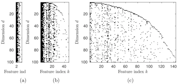
22 Chapter 2: Machine and Feature Learning Fundamentals 2 20 40 60 80 100 20 40 20 40 60 80 100 20 40 60 80 100 120 140 20 40 60 80 100 (a) (b) (c)
Figure 2.4. Different activation matrices obtained by sampling from the Indian Buffet Process with varying hyperparameter βa and fixed αa = 10, (a) βa = 0.2, (b) βa = 1,
and (c)βa = 5. The sparsity is increased withβa, resulting in more sampled features.
From the expression for the number of active features, ¯K+, it becomes apparent how the hyperparametersαaandβainfluence the number of active features. The probability
that an element in A∞ is active increases with both αa and βa. At the same time, the
expected number of active features grows linearly withαa, yielding sparse realizations.
Consequently, αa controls the number of active features. In contrast,βa has only little
effect on the number of active features. In particular, for βa → ∞, we obtain ¯K+ =
αaD, showing that the expected number of active features becomes independent of βa
for largeβa. Thus,βa can be understood as controlling the density of the realizations.
This is illustrated in Fig. 2.4.
Though the IBP models an infinite number of features, the number of active features is finite due to the sparsity assumption. Since we only need to store the active features in memory, the realizations are finite-sized matrices. Depending on the choice of the hyperparameters, the realizations can be sparse as well as dense.
2.3.3.2 Sampling from the Indian Buffet Process
Samples of feature representations are easily obtained by sampling from Eq. (2.11). For this, a Gibbs sampler [78] is used with a subsequent ordering of the activations. From the finite model in Eq. (2.10), the conditional for sampling the (k, d)th element
2.3 Feature Learning and Low-Dimensional Representations 23 of A, ak,d can be derived as [78] P(ad,k= 1|ak\d) = mk\d+αaKβa D+ αaβa K +βa−1 ,
whereak\dis the kth column ofA withoutak,d and mk\d is the sum over the elements
of ak\d. Considering the limit for K → ∞ results in [78]
P(a∞,d,k = 1|a∞,k\d) =
m∞,k\d
D+βa−1
.
Note that there is a certain probability that each element of the observation, indexed by
d,d= 1, . . . , D, has been generated by a feature that has not been inferred yet. Assum-ing exchangeability, the orderAssum-ing of the variables a∞,d,k becomes irrelevant [15]. Thus,
each element can be considered as the last being sampled such that the probability of activatingK0
+ new features for the dth element is independent of its index [78],
P(K+0 | −)∼PoissonK+ αaβa βa+D−1 , (2.12)
where the bar symbol (−) refers to all variables except K0
+.
In summary, samplingAworks as follows. We seta∞,d,kto one with probability
m∞,k\d
D+βa−1.
With probability P(K0
+| −), we add K+0 elements to the dth row of A. After having iterated over all active rows, a proposal is made to remove all columns that contain zero entries only, resulting in a sample of a binary matrix withK+ active rows, i.e.,K+ features.
Note that the samples generated by means of this algorithm need to be ordered if we want to sample feature class representations from the distribution in Eq. (2.11). The ordering can be achieved by means of the lof-operator described in [79] that sorts the columns of the transposed of A∞ into a left-ordered form (lof).
2.3.3.3 Sampling the Hyperparameters αa and βa
The hyperparameters αa and βa can be considered as Gamma distributed variables
with their own hyperparameters, h(1)αA, h
(2) αA, h (1) βA and h (2) βA [75], i.e., p(αa) = Gaαa h (1) αA, h (2) αA , p(βa) = Gaβa h(1)β A, h (2) βA .
24 Chapter 2: Machine and Feature Learning Fundamentals
The conditional of αa is given as [75]
p(αa| −) = Gaαa K+h (1) αA, D X d=1 βa βa+d−1 +h(2) αA ! ,
which can be sampled from efficiently. Since the likelihood and the prior ofβa are not
conjugate, we use a Metropolis step with the prior ofβa as proposal distribution. The
acceptance ratio rβa is then given as [75]
rβa = p(βa0| −) p(βa| −) = P(A|αa, βa 0 ) P(A|αa, βa) , where βa 0
denotes the proposed value.
2.4
Clustering and Classification
In this section, we revisit different clustering and classification methods that are utilized in Chapter 3. First, spectral clustering is briefly explained which we consider in the proposed band selection algorithm in Section 3.3. Second, the k-Nearest Neighbor (KNN) and the SVM classifier are introduced. Both classifiers are used for evaluation throughout Chapter 3.
2.4.1
Spectral Clustering
Many clustering algorithms such ask-means [80,81] or Expectation Maximization (EM) [82] for Gaussian mixture models pose strong assumptions on the distribution of the observations, which in practice may not hold and therefore lead to poor results. An alternative is the graph cut algorithm that has demonstrated accurate clustering re-sults in many image processing problems [83]. For image segmentation, the graph cut assumes a graph-based representation of the image, where the nodes are the elements of the image and the edges represent the affinities between the elements (high values indicate a high similarity between nodes). A sink and a source need to be defined, which represent pixels belonging to separate segments. According to the max-flow min-cut theorem [84], cutting the graph along the maximum flow between sink and source minimizes the energy and yields the segmentation result [83].
However, graph cut suffers from the problem that the sizes of the resulting clusters can be heavily unbalanced. Normalized cuts [85] overcome this problem by normalizing the
2.4 Clustering and Classification 25
cut by the volume of the segments. However, minimizing normalized cuts is an NP-complete problem [85]. A relaxation of normalized cuts is given by Spectral Clustering (SC) [86].
In the following, we briefly describe self-tuning SC [86, 87]. Let zn ∈ RD×1, with
n= 1, . . . , Nz, denoteNz D-dimensional observations that shall be clustered. For this, the normalized graph Laplacian, LSC, is defined [86],
LSC=D
−1/2 SC ASCD
−1/2 SC ,
whereASC is anNz×Nz matrix that describes the affinities between all features. The affinity between thenth and mth observation is defined as
aSC,n,m = exp{−
1
γ2 SC
kzn−zmk22} for n 6=m, (2.13) with γSC denoting a scaling factor. The self-affinities,aSC,n,n, n= 1, . . . , Nz, are set to
zero. The values of the diagonal matrix DSC are computed as the sums over the rows of ASC. Due to the nonlinearity in Eq. (2.13), scaling the observed data is crucial for successful clustering. We provide more details on this issue in Section 2.4.3.2.
Ideally, the number of clusters of the observations is given by the number of eigenvalues of the graph Laplacian that are equal to one [88]. In practice, due to noise and modeling errors, many eigenvalues may take values close to one, making a clear decision difficult. Thus, one resorts to setting KSC to the number of eigenvalues exceeding a predefined threshold. Stacking the corresponding KSC eigenvectors yields the transformed obser-vations VSC ∈ RNz×KSC. A conventional clustering algorithm, such as k-means, can then be used to cluster the transformed observations contained in the rows ofVSC. The value of the scaling factor, γSC, and the number of final clusters, KSC, have a strong impact on the result. Perona and Zelnik-Manor [87] present an efficient method to estimate local scales and a suitable number of clusters. A local scale, γSC,n, n =
1, . . . , Nz, can be considered as the distance between zn and its kth nearest neighbor
where k is determined by the dimension of the observation vector [87]. The affinity in Eq. (2.13) is then reformulated as
˜
aSC,n,m= exp{−
1
γSC,nγSC,mk
zn−zmk22},
with n = 1, . . . , Nz and m = 1, . . . , Nz. In order to estimate the number of clusters,
K, Perona and Zelnik-Manor [87] propose a cost function that aims at aligning VSC to the canonical coordinate system. Minimizing this cost function with respect to a rotation matrix implicitly yields the number of clusters. For details, we refer the reader to [87, 89, 90].


![Figure 4.2. Signatures selected from the USGS spectral library [165]. For the simula- simula-tions, the first K signatures are considered as the endmembers of the simulated hyper-spectral image](https://thumb-us.123doks.com/thumbv2/123dok_us/9235677.2808345/79.892.147.769.127.959/signatures-selected-spectral-signatures-considered-endmembers-simulated-spectral.webp)
