Partly Conditional Estimation of the Effect of a Time-Dependent
Factor in the Presence of Dependent Censoring
Qi Gong,1 Douglas E. Schaubel2,*
1Amgen, 1120 Veterans Blvd., South San Francisco, California 94080, U.S.A.
2Department of Biostatistics, University of Michigan, Ann Arbor, Michigan 48109-2029, U.S.A.
∗email:[email protected]
Summary. We propose semiparametric methods for estimating the effect of a time-dependent covariate on treatment-free survival. The data structure of interest consists of a longitudinal sequence of measurements and a potentially censored sur-vival time. The factor of interest is time-dependent. Treatment-free sursur-vival is of interest and is dependently censored by the receipt of treatment. Patients may be removed from consideration for treatment, temporarily or permanently. The pro-posed methods combine landmark analysis and partly conditional hazard regression. A set of calendar time cross-sections is specified, and survival time (from cross-section date) is modeled through weighted Cox regression. The assumed model for death is marginal in the sense that time-varying covariates are taken as fixed at each landmark, with the mortality hazard function implicitly averaging across future covariate trajectories. Dependent censoring is overcome by a variant of inverse probability of censoring weighting (IPCW). The proposed estimators are shown to be consistent and asymptotically normal, with consistent covariance estimators provided. Simulation studies reveal that the proposed estimation procedures are appro-priate for practical use. We apply the proposed methods to pre-transplant mortality among end-stage liver disease (ESLD) patients.
Key words: Dependent censoring; Inverse weighting; Landmark analysis; Longitudinal data; Proportional hazards regres-sion; Survival analysis; Time axis.
1. Introduction
Longitudinal and survival data are often observed simulta-neously in biomedical studies. For instance, measurements related to patient health may be collected over time as a longi-tudinal process during the course of a patient’s disease, while time to a failure event (e.g., death) is of chief interest. In-formation on time-varying covariates is usually collected at multiple follow-up times through the time to the event. For example, the number of CD4-lymphocyte counts is frequently employed as a surrogate marker for HIV; the glomerular fil-tration rate has been utilized as an indicator of kidney failure; the model for end-stage liver disease (MELD) score (Wiesner et al., 2001) is a very sensitive indicator of liver dysfunction among end-stage liver disease (ESLD) patients. In particular, the liver failure setting is the motivation for the methods we propose in this report.
It is often of interest to estimate the effect on survival time of a time-dependent factor hypothesized to be an important indicator for disease progression. In many practical applica-tions, there are actually two important time axes; follow-up time (e.g., time since diagnosis) and calendar time. The latter is important in settings wherein clinical decisions are made in calendar time. For example, in the organ transplant setting, a deceased-donor liver becomes available for allocation on a particular calendar date, and current allocation policy implies that the liver should be offered to the patient predicted to die soonest in the absence of a liver transplant. It makes sense to
structure the survival model in accordance with the research question. Hence, the most relevant time scale is time from that calendar date forward, and the cross-section of patients of interest (i.e., those transplant-eligible on that date) have various lengths of prior follow-up time. Covariate information to be used in the model would then include that observed up until the calendar date. Since future covariate information is not known, it is desirable for the model to implicitly average over future covariate paths. Models which condition on only part of the covariate history have been termed “partly condi-tional”; for example, Pepe and Couper (1997) and Zheng and Heagerty (2005).
To jointly model survival and longitudinal data, a re-gression model for the time dependent covariate process is usually adopted; for example, Tsiatis, Degruttola, and Wulf-sohn (1995); Henderson, Diggle, and Dobson (1997); Xu and Zeger (2001); Song, Davidian, and Tsiatis (2002); and Taylor (2011). In joint modeling of longitudinal/survival data, valid inference on the time-to-event component generally requires that the longitudinal process be modeled accurately, which is difficult to accomplish and may be cumbersome to carry out in many cases (including our motivating example). Moreo-ver, joint modeling approaches typically involve a (“fully”) conditional model of the death hazard as a function of the covariate at timet. In practice, such an approach may be in-consistent with the investigator’s objectives. For example, in the liver failure setting, it is of interest to determine which
of several patients awaiting liver transplantation will die soo-nest in the absence of a transplant; that is, based on each patient’s history up until that date, and averaging over the possible scenarios that could subsequently occur without a transplant.
Zheng and Heagerty (2005) proposed a partly conditional model applicable to some settings like that described in the preceding paragraph. Typically in modeling survival data, the event time, Di, is from study entry (marking the beginning
of follow-up) to the occurrence of the failure event. Zheng and Heagerty (2005) modeled survival time from measure-ment; that is, (Di−Si), withSidenoting measurement time.
The method of Zheng and Heagerty (2005) is referred as partly conditional since the hazard function being modeled (i.e., that of Di−Si) only conditions on the covariate
his-tory through time Si, rather than the full covariate history.
The time-varying covariate is “frozen” at each measurement time, as opposed to using information on {t:t > Si}. There
would typically be multiple event times for the same sub-ject, each corresponding to a different measurement time. The authors approach this element of the data structure through a multivariate survival analysis framework analogous to Wei, Lin, and Weissfeld (1989). The method does not re-quire modeling the longitudinal covariate process and there is no imposed dependence structure between different survi-val times from the same individual. With respect to related work, Van Houwelingen (2007) proposed a landmark model based on the partly conditional method. In this case, the time clock is not reset to zero every time a measurement is taken.
Existing partly conditional methods require that censoring be independent of death time. However, dependent censoring frequently occurs in observational studies. A particular case is when survival in the absence of treatment (hereafter re-ferred to as treatment-free survival) is of interest and both death and treatment assignment depend on the same time-varying covariates. If the model being fitted had conditioned on the entire history of the time-dependent covariates, then independent censoring could be assumed. However, since land-mark methods freeze the time-varying measurement at the landmark time, hence only using part of the covariate history, dependent censoring can result due to the mutual correla-tion between future treatment assignment date, treatment-free death hazard, and the portion of the covariate process occurring after the landmark time. Naturally, dependent cen-soring can result in biased estimation.
As stated previously, the data which motivated our cur-rent research arise from the liver failure setting. The preferred method of treatment for liver failure is deceased-donor liver transplantation. There are thousands more patients awaiting liver transplantation than there are deceased-donor livers. As a result, patients requiring liver transplantation who are dee-med dee-medically suitable are placed on a liver transplant wai-ting list. Currently in the United States, the guiding prin-ciple in prioritizing patients for liver transplantation is that patients who are predicted to die the soonest without a trans-plant should be given the highest priority for transtrans-plantation. Patients with acute liver disease (known as Status 1 patients) have the highest priority for liver transplantation and, hence, are placed at the top of the wait list. They are followed by
chronic liver failure patients, who are sequenced in decreasing order of MELD score. Note that MELD scores are updated over time, such that MELD is a time dependent process. In addition, if a patient becomes too sick, then he/she is remo-ved from the transplant waiting list. Or, inactive status can be issued but possibly canceled afterward. During an inac-tive period, the patient is not eligible for transplantation and will not receive offers of deceased-donor livers. In practice, it is required that an available donor liver be allocated based on information up until (and not beyond) the calendar date of procurement; analogous to the covariate information being frozen. In reality, subsequent liver allocation will be based on updated MELD scores observed after that calendar date. The-refore, although it is clear that liver transplantation censors pre-transplant death, such censoring amounts to dependent censoring in the context of a partly conditional model using landmark methods.
In this report, we propose landmark methods featuring a partly conditional model to estimate the effect of a time-dependent covariate, in the presence of time-dependent censoring. Inverse probability of censoring weighting (IPCW; Robins and Rotnitzky, 1992; Robins and Finkelstein, 2000) is used to obtain consistent estimators in the presence of dependent censoring. To increase precision, we propose two weight stabi-lizers that are different than those in the existing IPCW lite-rature. Each landmark is based on a common calendar date, not follow-up time, consistent with the motivating example. At each cross-section (landmark) date, patients who are under observation (alive, uncensored), untreated, and treatment-eligible are included in the cross-section. Survival time, with respect to a cross-section, is measured from the landmark date forward; such that the time clock is essentially reset to zero at each cross-section date. We assume that the baseline hazards may differ by cross-section, such that a stratified Cox model (1972) is appropriate.
The remainder of this article is organized as follows. In Section 2, we formulate the previously described characte-ristics of the motivating data structure, then describe the proposed methods. Asymptotic properties of the proposed es-timators are given in Section 3. A simulation study is pro-vided in Section 4. Results of applying the proposed me-thod to the afore-described liver failure data are presented in Section 5. In Section 6, we provide some concluding remarks and discussion. Asymptotic derivations are provided in the Web Appendix.
2. Proposed Methods
We begin by setting up the required notation. LetDi be the
treatment-free time to failure for subjecti, with i=1, . . . , n. We assume that Di may be censored at treatment time, Ti,
or independent censoring time, Ci, and therefore we define
the treatment-free observation time as Xi=min(Di, Ti, Ci).
We also define the associated indicators,i=I(Xi=Di) and
T
i =I(Xi=Ti), whereI(B)=1 when conditionBis true and
0 otherwise. We defineYi(t)=I(Xit). Each patient is
cha-racterized by a covariate vector,Zi(t), of which at least some
elements are time-varying. We let Ai(t) take value 1 if
pa-tient iis eligible to receive treatment as of follow-up timet, and 0 otherwise. Further, we define the covariate history as
Zi(t)= {Zi(s);s∈[0, t]} and the treatment-eligibility history
asAi(t)= {Ai(s); s∈[0, t]}.
We choose K cross-section dates (CSk, for k=1, . . . , K),
where the cross-section times represent calendar dates. The
{CS1, . . . , CSK}will typically be equally spaced, and the
ap-propriate number of cross-sections,K, will generally depend on the length of the observation period; issues to which we return in Section 6. LetSik denote the follow-up time of the
ith subject on the calendar date of thekth cross-section,CSk.
As we describe shortly, we will be modeling survival times from the cross-section dates, which essentially amounts to re-setting the time clock to 0 on each cross-section date. Cor-respondingly, sinceDi,Ti, andCiare measured in study time
(i.e., time since subject i started follow-up), we then define time since cross-section for death (Dik=Di−Sik), treatment
(Tik=Ti−Sik), and censoring (Cik=Ci−Sik). Thus, Dik,Tik,
and Cik are each measured from the kth cross-section date
forward.
With respect to cross-section k, one observes a vector for subject i, (Xik, ik, Tik), where Xik=min(Dik, Tik, Cik),
ik=I(Xik=Dik), and Tik=I(Xik=Tik). Note that, for a
censored subject,ik=Tik=0. For ease of presentation,
de-fineAik=Ai(Sik), an indicator for subjectibeing
treatment-eligible at the time of the kth cross-section. We now set up a modified version of counting process notation. In particu-lar, we letNik(t)=I(Xikt, ik=1)Aik, and write dNik(t)=
Nik(t−+dt)−Nik(t−) for the increment. The at risk process
is defined as Yik(t)=I(Xikt)Aik; that is, in addition to
subject i being alive and not treated as of time Sik (i.e.,
that Xi> Sik), to be included in thekth cross-section, it is
also required that the subject is treatment-eligible at time Sik (i.e., that Aik=1). However, if Aik=1, subject i is not
censored if he/she later becomes inactive at time t > Sik.
Thus, being treatment-eligible at time Sik is a cross-section
inclusion criterion, but subsequently becoming ineligible for treatment is not a censoring criterion. With respect to the treatment process, we define NT
i(t)=I(Xit, Ti =1). Note
that dNT
i(t)=Ai(t)dNiT(t), since treatment assignment can
only occur at time t for subject i if subjecti is treatment-eligible at timet.
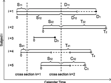
Figure 1 provides a graphical depiction of how each sub-ject’s treatment-free observation time is transformed into a set of time-since-cross-section dates. Five subjects are shown (i=1, . . . ,5) and two cross-sections (k=1,2). The five sub-jects begin follow-up at times which are staggered in calendar time. Subject 1 has failure timesD11corresponding to cross-sectionk=1 andD12with respect to cross-sectionk=2. Note that, even though subjecti=1 is deemed treatment-ineligible after cross-sectionk=2, the subsequent death is not censored. Subjecti=2 is treated (and therefore censored) at timeT22 with respect to cross-sectionk=2. Subjecti=3 is not inclu-ded in either cross-section sincei=3 starts and then finishes follow-up in between cross-sections. Subjecti=4 is included in cross-sectionk=1, then becomes treatment-ineligible until after cross-sectionk=2. Therefore,i=4 is included only in cross-sectionk=1. With respect to cross-sectionk=1, sub-ject i=4 is censored at treatment time, T41, as opposed to the time of treatment-ineligibility. Similarly, subjecti=5 is censored at timeC52, with respect to cross-sectionk=2, not
Figure 1. Examples of the relationship between cross-section time and follow-up time. Vertical dashed lines de-note cross-section dates (k=1,2), while horizontal dashed lines denote treatment-ineligible periods. Subjecti=1 is in-cluded in both cross-sectionsk=1 andk=2 and contributes death timesD11andD12to the analysis. Subjecti=2 is trea-ted at time T22 and, hence, censored (perhaps dependently) at that time. Subject i=3 is not included in either cross-section. Subjecti=4 is included in cross-section k=1, but not cross-sectionk=2 due to treatment-ineligibility. Subject i=5 is censored at time C52 from cross-section k=2. Note that subjectsi=1 andi=5 are not censored after becoming treatment-ineligible.
at the beginning of the treatment-ineligible period. The hazard function of interest can be expressed as
λik(t)=lim δ↓0 1 δP tDik< t+δ |Dikt, Aik=1,Zi(Sik),Ai(Sik), Sik . (1)
We letZik denote the pertinent covariate with respect to the
hazard function defined in (1). Essentially, we assume that the derived covariate, Zik captures all death hazard
predic-tors from the observed covariate and treatment-eligibility his-tories; specifically, that
λik(t|Zik, Aik=1,Zi(Sik),Ai(Sik), Sik)=λik(t|Zik, Aik=1).
Note that thetargument pertains to time after thekth cross-section date, with the covariate “frozen” at its cross-cross-section date value. The objective is to determine the relationship bet-ween the covariate (as known on thekth cross-section date) and future treatment-free survival time. Since the underlying goal is to determine what factors are associated with treat-ment urgency, only subjects who are treattreat-ment-eligible at the kth cross-section date are of interest; hence the conditioning on [Aik=1].
Death times are modeled using stratified Cox regression,
λik(t)=λ0k(t) exp{β0Zik}, (2)
where the baseline hazards are allowed to be cross-section-specific, although covariate effects are assumed to be equal across all cross-sections. We make the standard independent censoring assumption which, in the context of the observed data, is given by:
λik(t|Zi(Sik+t),Ai(Sik+t), Aik=1, Tik> t, Cik> t)
=λik(t|Zi(Sik+t),Ai(Sik+t), Aik=1). (3)
However, a model for Dik conditioning on onlyZik does not
incorporate{Zi(r);r∈(Sik, Sik+t)}or{Ai(r);r∈(Sik, Sik+t)}.
Generally, λik(t|Zik, Aik=1)=λik(t|Zik, Aik=1, Tik> t) due
to the correlation betweenTik andDik resulting from mutual
dependence on{Zi(r); r > Sik}and/or{Ai(r); r > Sik}. In this
sense, the assumption listed in (3) does not lead to parameter estimation for model (2) through unweighted methods.
We use a variant of IPCW to overcome the dependent cen-soring ofDikbyTik. The following treatment hazard model is
assumed, λTi(t)=Ai(t)λT0(t) exp θ0Zi(t) , (4)
where t is the time from study entry. As indicated in equa-tion (1), the treatment hazard is zero at times during which the patient is treatment-ineligible. Therefore, treatment hazards among eligible patients are assumed to be pro-portional. Similar to the presentation for model (2), the covariate in model (4) is written as Zi(t) for notational
convenience and, more generally, could depend on the co-variate and treatment-eligibility histories, Zi(t) and Ai(t),
respectively. We make a no-unmeasured-confounders type as-sumption with respect to treatment; that is, we assume that λT
i(t|Zi(t), Ai(t),Zi(Di),Ai(Di), Di)=λTi(t|Zi(t), Ai(t)).
The regression coefficient,θ0, is estimated byθ, as the root of the score function,
UT(θ)= n i=1 τ 0 Zi(t)−Z(t;θ) dNiT(t),
where τ is the largest observation time, Z(t;θ)= R(1)T (t;θ)/R (0) T (t;θ), andR (p) T (t;θ)=n−1 n i=1Ai(t)Yi(t)Zi(t)⊗p
exp{θZi(t)}forp=0,1,2, witha,a⊗0=1,a⊗1=a,a⊗2=aaT
for a vector, a. The Breslow estimator ofT
0(t) is given by T 0(t)=n−1 n i=1 t 0R (0) T (u;θ)−1dNiT(u).
The IPCW method allows us to obtain consistent estima-tors by weighting each subject’s experience by the inverse of (what can be thought of heuristically as) the probability of remaining untreated. In particular, the covariate effect, β0, can be estimated as the root of the stratified inverse-weighted
score function, U(β, W)= K k=1 n i=1 τk 0 Aik Zik−Zk(t;β, W) WikA(t)dNik(t), (5) where the weight function is given by WA
ik(t)=Yik(t) exp {T i(Sik+t)−Ti(Sik)} and Zk(t;β, W)=R (1) k (t;β, W)/ R(0)k (t;β, W), withRk(p)(t;β, W)=n−1n i=1AikWikA(t)Yik(t)Z⊗ p ik
exp(βZik) for p=0,1,2. The upper limit, τk, satisfies
P(Xikτk)>0 and in practice would usually be set to
max{Xik}. We refer to WikA(t) as the Type A weight. The
quantity does not constitute a stabilized weight (Robins and Finkelstein, 2000). However, the quantity can be thought of heuristically as a ratio of two probabilities, P(Ti> Sik+t|Ti> Sik)−1. From this angle, large values
of T
i(Sik+t) should, to at least some extent, coincide
with large values of T
i(Sik), such that the Type A weight
is less subject to wide variation, unlike the unstabilized weight in more traditional dependent censoring settings. We demonstrate in the Web Appendix that U(β0, W) from (5) has mean 0. Essentially, the zero mean pro-perty arises from E[WA
ik(t)dMik(t)|Zik, Aik=1]=0, where
dMik(t)=dNik(t)−Yik(t)dik(t).
Additionally, it can be argued that E[WA
ik(t)dMik(t)g(Zik)|
Zik, Aik=1]=0, whereg(·)∈Ris a deterministic function of
the covariate,Zik, used in model (2). Often,g(Zik) is chosen to
be a probability, since the unstabilized version of the weight is the reciprocal of a probability. Along this train of thought, we define the Type B weight,
WikB(t)=Yik(t) exp{T i(Sik+t)} exp{T i(Sik)}exp{Tik(t)} , whereT ik(t)= t 0λ T ik(u)du, with λT ik(t)=lim δ↓0 1 δP tTik< t+δ|Tikt,Zik, Aik=1 . (6)
which we represent through the model, λT
ik(t)=AikλT0k(t) exp{θ1Zik}. (7)
Consistent with the death hazard, λD
ik(t), given in (1), the
double subscripting in (6) corresponds to the time scale being time from cross-section, and conditionality on [Zik, Aik=1].
One can interpret λT
ik(t) as the hazard function for
treat-ment, with time measured from Sik onward, among patients
alive, untreated, and treatment-eligible at time Sik. We can
re-express the Type B weight asWB
ik(t)=WikA(t) exp{−Tik(t)},
with exp{−T
ik(t)}reflecting the conditional probability of
re-maining untreatedttime units afterSik, given untreated and
treatment-eligible at timeSik. From this perspective, the Type
B weight can be viewed as stabilized, since its numerator and denominator are both akin to conditional probabilities. Note that we do not expect (7) to be a correct model; its purpose is to provide a reasonable version ofg(Zik) to be incorporated
into the weight function as a stabilizer. In contrast, consistent estimation ofβ0 does require that model (4) be correct.
Another weight which can be used is the Type C weight, WikC(t)=Yik(t) exp
Ti(Sik+t)
, (8)
which is reminiscent of the unstabilized weight in more tra-ditional dependent censoring settings. In particular, inverse weighting the data (without a view to the model of inter-est) would lead to WC
ik(t). However, in our set-up, the Type
A weight is actually the “raw” version of the weight; in the sense that theWA
ik(t) function is defined specifically such that
E[WA
ik(t)dMik(t)|Zik, Aik=1]=0, resulting on (5) having mean
zero (see the Web Appendix for associated details). Therefore, we could only expect that E[WC
ik(t)dMik(t)|Zik, Aik=1]=0 if
we can expressWC
ik(t) as the product ofWikA(t) and some
sui-tably defined g(Zik). From this perspective, setting g(Zik)=
exp{T
i(Sik)}, and henceWikC(t)=WikA(t) exp{Ti(Sik)}, reveals
that the Type C weight actually amounts to dividing the “raw” weight function by a probability. Viewed this way, WC
ik(t) should lead, if anything, to increased variance. Our
thoughts regarding the Type A, B, and C weights are asses-sed numerically in Section 4.
3. Asymptotic Properties
We assume that the random vectors {Xi, i, Ti,Zi(Xi),
Ai(Xi)}, for i=1. . . n, are independent and identically
distributed, withZi(t) bounded fort∈(0, τ], whereτsatisfies
P(Xiτ)>0. We summarize the asymptotic properties
of the proposed methods in the following theorem. The regularity conditions are listed in the Web Appendix.
THEOREM 1: Under certain regularity conditions,
n1/2(β−β
0) converges asymptotically to a zero-mean
Gaussian process with covariance function E[ϕiϕi], where
{ϕ1, . . . , ϕn}are i.i.d. with mean 0 asymptotically, with
ϕi=(β0)− 1 K k=1 Aik τk 0 {Zik−zk(t;β0, W)}W A ik(t)dMik(t) +H(t;β0, W)T(θ0)−1UiT(θ0) + τk Sik G(t, τ;β0)rT(0)(t;θ0)− 1d MTi(t) , where dMT i(t)=dN T i(t)−Ai(t)Yi(t) exp{θZi(t)}T0(t), zk(t;β, W)=r (1) k (t;β, W)/r (0) k (t;β, W), z(t;θ)=r(1)T (t;θ)/r(0)T (t;θ), r(kp)(t;β, W)=E[AikWikA(t)Yik(t)Z⊗ p ik exp(βZik)], p=0,1,2, rT(p)(t;θ)=E[Ai(t)Yi(t)Zi(t)⊗pexp{θZi(t)}], p=0,1,2,
with (β), H(t;β, W),T(θ),UiT(θ), andG(t1, t2;β) defined in the Web Appendix.
The covariance can be estimated consistently by n−1n
i=1ϕiϕi, where ϕi is obtained by replacing all
li-miting values in ϕi by their empirical counterparts. A
proof of Theorem 1 is provided in the Web Appendix. The proof proceeds by demonstrating that, asymptotically, n1/2(β−β
0)=n−1/2 n
i=1ϕi+op(1) through a sequence of Taylor series expansions.
Note that subjects (i=1, . . . , n) are assumed to be in-dependent. However, no independence assumption is made regarding the cross-section-specific contributions of a given subject; the dependence structure for the within-subject score function contributions being left unspecified. Since we do not model the within-subject correlation explicitly, our approach is analogous to generalized estimating equations (GEE) with a working independence assumption (Liang and Zeger, 1986). It is well-established in the GEE literature that, so long as the model for the marginal mean is correct, one need not model the within-subject correlation structure accurately in order to obtain a consistent estimator of the regression coefficient for the mean model.
The proof of Theorem 1 is developed in the context of the Type A weight, WA
ik(t)=Yik(t) exp{Ti(Sik+t)−Ti(Sik)}. In
practice, a stabilized version would usually be preferred. As implied by Theorem 1, the computation of the variance is quite complicated, and is more complicated with the Type B weight. Such considerations motivate a computationally sim-pler form for the variance estimator. One such simplification involves treating the weight (be it WA
ik(t), W B
ik(t), or W C ik(t))
as fixed; in which case the variance estimator simplifies to n−1n i=1ϕi∗ϕ∗ i, where ϕ∗i =(β)− 1 K k=1 Aik τk 0 Zik−Zk(t;β,W) Wik(t)dMik(t).(9)
This simplified variance estimator can be calculated using Cox regression software that allows weights and a robust variance estimator; for example, proc phreg in SAS, coxph in R. Perti-nent SAS code is available from the first author upon request.
4. Simulations
We modify the algorithm developed by Zheng and Heagerty (2005) to generate data which follow a partly conditio-nal proportioconditio-nal hazards model. We first generate a binary treatment group indicator, Zia, taking values 0 and 1 with
probability 0.5. A longitudinal marker, Zi(Sik), measured
at a common set of cross-section dates (CS1, CS2, . . . , CSK)
is then constructed. To generate data [Di, Zia,Zib] where
Zib=vec{Zi(Sik)}, we first createZib0=bi+
K
k=1log(Vik)/γ2,
where bi∼N(μ, σ2) and the Vik are independent positive
stable variates with index ρ (Samorodnitsky and Taqqu, 1994). A pre-treatment death timeDi, is then generated with
hazardλi(t)=V
1/ρ
i0 λ0(t) exp{γ1Zia+γ2Zib0},whereVi0∼P(ρ) and is independent of Vik, with0(t)=(t/a)1/ρ
2
and ais a constant. Let Zi(Sik)=Zib0−log(Vik)/γ2. The death hazard
is then written as λi(t)=V 1/ρ i0 λ0(t) exp γ1Zia+γ2Zi(Sik)+log(Vik) . (10)
Subjectienters the study on calendar dateLi, whereLiis
a Uniform(0,b) variate. Treatment time,Ti, is generated from
the proportional hazards model, λT i(t)=λ T 0(t) exp θ01Zia+θ02I(t > Ri) , (11) where λT 0(t)=d3, θ0=(θ01, θ02), and Ri is time of
treatment-ineligibility which is generated with hazardλR i(t)=
λR
0(t) exp{d1Vi0}, withλ0R(t)=1/d2. Thus,RiandDiare
posi-tively correlated, which is a reflection of the data which mo-tivated the proposed methods. Note that treatment time and pre-treatment death time, Ti, and Di, are dependent since
both depend on time of treatment ineligibility,Ri.
To see that the prescribed set-up yields proportional ha-zards, integrating both sides of model (4), gives
i(t)=V 1/ρ i0 0(t) exp γ1Zia+γ2Zi(Sik) Vik,
such that the pre-treatment survival function is given by exp{−i(t)} =exp −0(t) exp{γ1Zia+γ2Zi(Sik)}VikV 1/ρ i0 . Transforming the time scale to reflect time since cross-section, definetk=t−Sik. Then, take the expectation with respect to
Vikfirst and using the properties of the positive stable
distri-bution, we have exp−i(tk|Zia, Zi(Sik), Di> Sik, Vi0) = exp [0(t) exp{γ1Zia+γ2Zi(Sik)}V 1/ρ i0 ]ρ cos(πρ/2) .
Then, taking the expectation with respect toVi0, we have
exp−i(tk|Zia, Zi(Sik), Di> Sik) = exp −0(t)ρ2 exp{ρ2γ 1Zia+ρ2γ2Zi(Sik)} cos(πρ/2)(ρ+1) ,
which implies the following equation after taking logarithm and negative of both sides
i(tk|Zia, Zi(Sik), Di> Sik) = 0(t) ρ2 expρ2γ 1Zia+ρ2γ2Zi(Sik) cos(πρ/2)(ρ+1) .
Differentiating with respect totk,
λi(tk|Zia, Zi(Sik), Di> Sik)= λ0(tk+Sik)ρ2{0(tk+Sik)}(ρ 2−1) cos(πρ/2)(ρ+1) expρ2γ 1Zia+ρ2γ2Zi(Sik) . Using this construction, the hazard for Dik=Di−Sik
will generally depend on Sik and therefore stratified
mo-dels similar to those considered by Wei et al. (1989) would be appropriate. With0(t)=(t/a)1/ρ
2 ,λ0(tk+Sik)ρ2{0(tk+ Sik)}(ρ 2−1) =1/a, we obtain λi(tk|Zia, Zi(Sik), Di> Sik) = exp ρ2γ 1Zia+ρ2γ2Zi(Sik) [acos(πρ/2)(ρ+1)] . If we define λik(t;Sik)=λi(tk|Zia, Zi(Sik), Di> Sik), λ0k(t)= [acos(πρ/2)(ρ+1)]−1 andβ 0=(β01, β02)=(ρ2γ1, ρ2γ2), then the proportional hazard model on treatment-free survival is achieved, λik(t;Sik)=λ0k(t) exp β01Zia+β02Zi(Sik) . (12) After generating the data, we only include for analysis those Zi(Sik) withLi< Sik<min(Xi, Ri). Data pertaining to
survi-val time since cross-section{Xik, ik, Zia, Zi(Sik)}is used to fit
model (6), with time-to-treatment data {Xi, Ti, Zia,Zi(Xi)}
used to fit model (5).
We evaluate samples with n=1000 subjects and obtain 10%,20%, and 40% censoring by varying a from 104 to 4×10⁷. The value of d
2 varies from 300 to 3000, resul-ting in ineligibility rates from 10% to 30%. There are K= 10 cross-section dates. We set b=500, [θ01, θ02]=[−1,−1], μ=18, σ=1, [γ1, γ2]=[−1,−0.5],[−0.5,−0.25],[0,0], d1= d3=0.001, with CSk=100×k. For all our simulated
situa-tions, 1000 Monte Carlo data sets are used. We present results using ρ=0.8, thus [β01, β02]=[−0.64,−0.32] when [γ1, γ2]=[−1,−0.5]. With the number of cross-sections set to K=10, the average number of cross-sections per subject is 0.7–2.4, depending on the censoring level. We apply the sim-plified variance estimate which treats the estimated weights as fixed; that is, as given in (9).
Table 1 presents simulation results based on the Type A weight, while Tables 2 and 3 present results for Type B and Type C, respectively. Estimates ofβ0appear to be consistent based on all weights. The variance of the Type B estimator is smaller than that of Type A, which is likely the result of the added stabilizer. Coverage probabilities using the proposed (simplified) variance estimator are close to the nominal 95% level, with those of the Type B estimator being slightly higher than those of Type A. The variance of the Type C estimator appears to be greater than that of Type A, consistent with our comments in Section 2 that the Type C weight can be viewed as the result of dividing a ratio of probabilities (i.e., WA
ik(t), which should be fairly stable) by another probability.
5. Data Analysis
We applied the proposed methods in order to compare pre-transplant mortality between acute and chronic ESLD pa-tients. Data were obtained from the Scientific Registry of Transplant Recipients (SRTR), a national population-based organ transplant registry. The study population included pa-tients initially wait listed for deceased-donor liver transplan-tation between March 1, 2002 and December 31, 2009 in Uni-ted States. Only patients age ≥18 at listing and not pre-viously transplanted (i.e., not repeat transplant candidates) were included in the study population. Cross-section dates were chosen every 7 days from March 1, 2002 to December 31,
Table 1
Simulation results forβcomputed using Type A WeightWA
ik(t);n=1000
β01 β02
Censored (%) β∗01 Bias ESE ASE CP β∗02 Bias ESE ASE CP
10 −0.64 −0.009 0.132 0.125 0.93 −0.32 −0.001 0.020 0.020 0.95 20 −0.004 0.143 0.128 0.92 −0.002 0.020 0.019 0.94 40 −0.008 0.145 0.129 0.93 0.001 0.018 0.018 0.94 10 −0.32 0.002 0.146 0.132 0.93 −0.16 0.001 0.013 0.012 0.93 20 −0.004 0.140 0.129 0.92 −0.001 0.010 0.010 0.94 40 −0.001 0.144 0.130 0.92 −0.001 0.010 0.009 0.94 10 0 0.001 0.140 0.130 0.93 −10−4∗∗ −0.003 0.048 0.044 0.94 20 −0.002 0.136 0.127 0.94 −0.001 0.042 0.041 0.95 40 −0.007 0.143 0.128 0.93 −0.002 0.038 0.036 0.94 ∗β 0=(β01, β02)=(ρ2γ1, ρ2γ2),whereρ=0.8.
∗∗ The Bias, ESE, and ASE shown in this block are in 10−4 scale.
Table 2
Simulation results forβcomputed using Type B Weight given in (4);n=1000
β01 β02
Censored (%) β∗01 Bias ESE ASE CP β∗02 Bias ESE ASE CP
10 −0.64 0.004 0.130 0.121 0.94 −0.32 −0.001 0.021 0.020 0.94 20 −0.008 0.121 0.116 0.94 −0.001 0.018 0.018 0.95 40 −0.008 0.113 0.112 0.94 −0.001 0.016 0.016 0.95 10 −0.32 −0.005 0.136 0.130 0.94 −0.16 −0.001 0.012 0.011 0.94 20 −0.005 0.122 0.117 0.94 −0.001 0.010 0.009 0.94 40 0.003 0.112 0.109 0.93 −0.001 0.008 0.008 0.94 10 0 0.005 0.135 0.126 0.93 −10−4∗∗ −0.001 0.044 0.043 0.94 20 −0.005 0.123 0.118 0.94 −0.002 0.041 0.038 0.94 40 0.004 0.109 0.109 0.95 −0.002 0.031 0.031 0.95 ∗β 0=(β01, β02)=(ρ2γ1, ρ2γ2),whereρ=0.8.
∗∗ The Bias, ESE, and ASE shown in this block are in 10−4 scale.
Table 3
Simulation results forβcomputed using Type C Weight given in (5);n=1000
β01 β02
Censored (%) β∗01 Bias ESE ASE CP β∗02 Bias ESE ASE CP
10 −0.64 0.002 0.142 0.129 0.93 −0.32 −0.002 0.022 0.021 0.94 20 −0.005 0.144 0.136 0.93 −0.001 0.022 0.020 0.92 40 −0.010 0.159 0.136 0.90 −0.002 0.020 0.019 0.94 10 −0.32 −0.003 0.146 0.135 0.94 −0.16 −0.001 0.012 0.012 0.94 20 −0.012 0.154 0.138 0.91 −0.001 0.012 0.011 0.92 40 −0.003 0.157 0.138 0.91 −0.001 0.011 0.010 0.94 10 0 −0.008 0.153 0.136 0.92 −10−4∗∗ −0.002 0.047 0.046 0.94 20 −0.001 0.146 0.134 0.92 −0.002 0.045 0.043 0.94 40 0.007 0.155 0.137 0.92 −0.002 0.042 0.040 0.93 ∗β 0=(β01, β02)=(ρ2γ1, ρ2γ2),whereρ=0.8.
2009, such that there wereK=409 cross-sections in all. At any given cross-section date, any subject who was still on the wait-list (not inactive and not removed) was included in the cross-section since, in practice, patients who got removed or were made inactive were no longer eligible to receive offers for deceased-donor livers. Given the objectives of our analysis, it is appropriate to compare only patients who, in a given cross-section date, are in fact eligible to receive a liver transplant. However, after being included into a given cross-section, such patients are not censored if they are subsequently deactivated or removed from the wait-list. Deactivation and removal (and the associated death that may follow) are potential conse-quences of not receiving a liver transplant. For the death mo-del, the failure time was defined from the date of cross-section to the date of the earliest of death, transplant, or censoring.
In order to construct the IPCW weight,T
i(t) was
estima-ted based on a time-dependent Cox model in which transplant was the event. For the time-to-transplant model, timetstarts from the beginning of the follow-up (the date of wait listing), as opposed to cross-section time. The model was stratified, such that λT ir(t)=Ai(t)λT0r(t) exp θ0Zi(t) ,
where the subscriptr=1, . . . ,11 stands for region. The pre-sence of the indicator,Ai(t), reflects the fact that a patient’s
time while inactive or removed does not contribute to the es-timation of θ0 or T0r(t). The patient level covariate, Zi(t),
included MELD score, Status 1, albumin, age, gender, race, diagnosis of Hepatitis C, body mass index, diabetes, hospi-talization, blood type, dialysis within prior week, encephalo-pathy, ascites, and serum creatinine. Among the covariates in this list, MELD score, albumin, dialysis, encephalopathy, ascites, and serum creatinine were time-dependent.
We evaluated several different versions of weight, including Wikr(t)=Yikr(t) (unweighted), WikrA(t)=Yikr(t) exp
T ikr(t+ Sik)−Tikr(Sik) ,WB ikr(t), andW C
ikr(t). Some very large values of
the weight function occurred, even forWB
ikr(t). Since we found
that 99% of weights were <10, weights were then capped at 10.
The model of primary interest, the pre-transplant death model, was also stratified
λikr(t)=λ0kr(t) exp
β0Zik
,
where the subscript r=1, . . . ,11 stands for region and k= 1, . . . ,409 stands for cross-section. The cross-section-specific covariates,Zik, included albumin, age, gender, race, diagnosis,
body mass index, diabetes, hospitalization status at listing, previous malignancy; as well as the covariate of chief inter-est, MELD score (21–23, 24–26, 27–29, 30–32, 33–35, 36–40), with each MELD category being compared to Status 1, the reference. Also included inZikwere average change in MELD
score (pertaining to the time interval between the date of listing and cross-section k date, and estimated using ordi-nary least squares) and average change in albumin (estimated analogously). Other elements included the percentage of time spent in inactive status, and percent of time receiving dialysis. Since 99% of MELD and albumin slope values before
cross-Table 4
Analysis of liver wait-list mortality (using Type B Weight)
Group β SE(β) eβ p-value Status 1 0 — 1 — MELD 21–23 0.05 0.267 1.05 0.87 MELD 24–26 0.18 0.272 1.20 0.50 MELD 27–29 0.52 0.276 1.68 0.06 MELD 30–32 0.25 0.334 1.29 0.45 MELD 33–35 0.96 0.301 2.62 0.001 MELD 36–40 0.95 0.306 2.58 0.002
sections fell in the [−1, 1] interval, the slopes were bounded by
−1 and 1. Our final sample consisted ofn=23,657 patients. Results based on the death model using the Type B weight are listed in Table 4. Relative to Status 1, pre-transplant mor-tality is 2.62 times as great for MELD 33–35 (p=0.001) and 2.58 times as great for MELD 36–40 (p=0.002).
Both unweighted and weighted results are listed in Table 5. After weighting the model, the parameter estimates of MELD group became larger, in each case. Similar to the findings from simulation studies, the standard errors in Table 5 were the lowest for the Type B weight, while those for Type C were the largest.
Supplementary analysis revealed that acute patients died very fast in the early stage. The Status 1 Kaplan–Meier curve initially dropped much more quickly than the survival curves for the MELD groups. However, the Status 1 survival curve leveled off eventually, while the survival curves for the MELD groups kept dropping.
6. Discussion
We propose semiparametric methods to estimate the effect of a time dependent covariate on treatment-free survival. Ptreatment death may be dependently censored by the re-ceipt of treatment, and subjects may experience periods of treatment-ineligibility. The proposed methods estimate the regression parameter of a partly conditional hazard model through landmark analysis and IPCW. The proposed estima-tors are demonstrated to be consistent and asymptotically normal, with consistent covariance estimators provided.
Zheng and Heagerty (2005) proposed partly conditional Cox regression methods. Van Houwelingen (2007) proposed landmark models based on partly conditional methods. In Zheng and Heagerty (2005), the time clock is re-set at co-variate measurement times, unlike our methods, wherein the clock is re-set at cross-section dates. Neither the Zheng and Heagerty (2005) or Van Houwelingen (2007) methods deal with dependent censoring or accommodate treatment ineligi-bility.
Comparisons of pre-transplant death rates between Status 1 and MELD patients have rarely been conducted; in part, since the assumption that Status 1 patients have the highest death rate is widely accepted by the liver transplant commu-nity. However, in a recent study (Sharma et al., 2012) using a traditional time-dependent model, death rates for patients with MELD≥40 were shown to be significantly higher than those of Status 1. Analysis shown in Section 5 based on the
Table 5
Analysis of liver wait-list mortality; comparison of results using different weights
Unweighted Type C Weight Type A Weight Type B Weight
Group β SE(β) β SE(β) β SE(β) β SE(β) Status 1 0 . 0 . 0 . 0 . MELD 21-23 −0.81 0.210 0.01 0.271 0.07 0.270 0.05 0.267 MELD 24-26 −0.75 0.215 −0.002 0.286 0.11 0.281 0.18 0.272 MELD 27-29 −0.29 0.220 0.31 0.287 0.42 0.283 0.52 0.276 MELD 30-32 −0.32 0.256 0.10 0.348 0.11 0.339 0.25 0.334 MELD 33-35 0.26 0.246 0.91 0.345 0.92 0.321 0.96 0.301 MELD 36-40 0.33 0.272 0.79 0.335 0.73 0.324 0.95 0.306
proposed methods show that MELD33 is associated with significantly higher pre-transplant mortality than Status 1.
Some discussion regarding the appropriate number of cross-sections,K, is in order. GreaterKgenerally results in a greater amount of information, although returns diminish since infor-mation overlaps among different cross-sections. Some guiding principles are as follows. First, it seems reasonable to make the cross-sections equally spaced. Second, it is preferable to select a “start” date (i.e., for cross-sectionk=1) that is easy to identify with (e.g., January 1, 2000) then fix the time in-terval between cross-sections thereafter (e.g., every 30 days). Third, the disincentive to choosing a larger number of cross-sections is largely computational burden. Choosing K cross-sections amounts to essentially stackingKdata sets together prior to analysis. For a given cross-section k, the covariate used in the death model,Zikis defined once per subject.
Ho-wever, each subject will typically contribute multiple records per cross-section since changes in the covariate and eligibi-lity status affect the subject’s inverse weight. In summary, we suggest picking an intuitive cross-section start date for k=1; making the cross-sections equally spaced; spacing the cross-section dates such that as many cross-sections as com-putationally feasible are used. One could argue that if an ap-propriate number of cross-sections is employed, then adding cross-sections will not alter the results for the death model meaningfully.
The proposed methods assume that the death hazards for the subgroups of interest are proportional. It would be use-ful to develop extensions of the proposed methods to target measures which do not require the proportional hazards as-sumption.
7. Supplementary Materials
Web Appendix A, referenced in Section 2, is available with this article at the Biometrics website on Wiley Online Library.
Acknowledgements
This work was supported in part by National Institutes of Health Grant 5R01 DK070869. The authors thank Jack Kalb-fleisch, Min Zhang, and Bob Merion for thoughtful comments on this report. The data reported here have been supplied by the Minneapolis Medical Research Foundation (MMRF) as the contractor for the Scientific Registry of Transplant
Reci-pients (SRTR). The interpretation and reporting of these data are the responsibility of the authors and in no way should be seen as an official policy of or interpretation by the SRTR or the U.S. Government. The authors also wish to thank the Coordinating Editor, Associate Editor, and two Referees for comments which considerably strengthened the manuscript.
References
Cox, D. R. (1972). Regression models and life-tables (with discus-sion).Journal of the Royal Statistical Society, Series B34, 187–220.
Henderson, R., Diggle, P., and Dobson, A. (1997). A joint model for survival and longitudinal data measured with error. Bio-metrics53, 330–339.
Liang, K.-Y. and Zeger, S. L. (1986). Longitudinal data analysis using generalized linear models.Biometrika73, 13–22. Pepe, M. S. and Couper, D. (1997). Modeling partly conditional
means with longitudinal data.Journal of the American Sta-tistical Association92, 991–998.
Robins, J. M. and Finkelstein, D. M. (2000). Correcting for non-compliance and dependent censoring in an AIDS clinical trial with inverse probability of censoring weighted (IPCW) log-rank tests.Biometrics56, 779–788.
Robins, J. M. and Rotnitzky, A. (1992). Recovery of informa-tion and adjustment for dependent censoring using surro-gate markers. In N. Jewell, K. Dietz, and B. Farewell, editors, AIDS Epidemiology—Methodological Issues, pages 297–331. Boston: Birkh¨auser.
Samorodnitsky, G. and Taqqu, M. S. (1994).Stable Non-Gaussian Random Processes, Stochastic Models with Infinite Va-riance. New York: Chapman and Hall.
Sharma, P., Schaubel, D. E., Gong, Q., Guidinger, M. K., and Me-rion, R. M. (2012). End-stage liver disease candidates at the highest MELD scores have higher waitlist mortality than Status 1A candidates.Hepatologypublished online.55, 192– 198.
Song, X., Davidian, M., and Tsiatis, A. A. (2002). A semipara-metric likelihood approach to joint modeling of longitudinal and time-to-event data.Biometrics58, 742–753.
Taylor, J. M. G. (2011). Discussion of predictive comparison of joint longitudinal-survival modeling: A case study illustra-ting compeillustra-ting approaches, by Hanson, Branscum and John-son.Lifetime Data Analysis1, 29–32.
Tsiatis, A. A., Degruttola, V., and Wulfsohn, M. S. (1995). Mode-ling the relationship of survival to longitudinal datameasu-red with error. Application to survival and CD4 counts in
patients with AIDS.Journal of American Statistical Asso-ciation90, 27–37.
Van Houwelingen, H. C. (2007). Dynamic prediction by landmar-king in event history analysis.Scandinavian Journal of Sta-tistics34, 70–85.
Wei, L. J., Lin, D. Y., and Weissfeld, L. (1989). Regression analy-sis of multivariate incomplete failure time data by modeling marginal distributions.Journal of the American Statistical Association84, 1065–1073.
Wiesner, R. H., McDiarmid, S. V., Kamath, P. S., Edwards, E. B. Malinchoc, M., Kremers, W. K., Krom, R. A. F.,
and Kim, W. R. (2001). MELD and PELD: Application of survival models to liver allocation.Liver Transplantation7, 567–580.
Xu, J. and Zeger, S. L. (2001). Joint analysis of longitudinal data comprising repeated measures and times to events.Applied Statistics50, 375–387.
Zheng, Y. Y. and Heagerty, P. J. (2005). Partly conditional survival models for longitudinal data.Biometrics61, 379–391.
Received December 2011. Revised December 2012. Accepted December 2012.