A Framework for Explicit Model Predictive Control using Adjustable Robust Optimization and Economic Optimization of an Industrial-Scale Sulfuric Acid Plant

(1)

A Framework for Explicit Model

Predictive Control using Adjustable

Robust Optimization and Economic

Optimization of an Industrial-Scale

Sulfuric Acid Plant

by

Manuel Alejandro Tejeda Iglesias

A thesis

presented to the University of Waterloo in fulfillment of the

thesis requirement for the degree of Master of Applied Science

in

Chemical Engineering

Waterloo, Ontario, Canada, 2018

(2)

Author's Declaration

I hereby declare that I am the sole author of this thesis. This is a true copy of the thesis, including any required final revisions, as accepted by my examiners.

(3)

Abstract

Optimization plays an important role in the operation of chemical engineering systems. Due to their typical size, different optimization tools and techniques are required to improve the efficiency in process operations. In this thesis, a mathematical tool is developed to address the issue of optimal control for linear systems under uncertainty. Also, a comprehensive plant model describing the behaviour of an industrial-scale Sulphuric Acid plant is developed to assist in identification of the optimal operating conditions under uncertainty

Model predictive control (MPC) is considered an attractive strategy for the optimal control of complex chemical engineering systems. Conventional MPC involves solving an optimization problem online to determine the control actions that minimize a performance criterion function. The high computational expense associated with conventional MPC may make its application challenging for large-scale systems. Explicit MPC has been developed to solve the optimization problem offline. In this work, adjustable robust optimization (ARO) is used to obtain the explicit solution to the MPC optimization problem offline for discrete-time linear time invariant systems with constraints on inputs and states. In the robust model formulation an uncertain additive time-varying error is introduced to account for model uncertainty resulting from plant-model mismatch caused by un-measurable disturbances or process nonlinearities. The explicit solution is an optimal time-varying sequence of feedback control laws for the control inputs parameterized by the system’s states. The control laws are evaluated in a time-varying manner when the process is online using state measurements. This study shows that the resulting control laws ensure the implemented control actions maintain the system states within their feasible region for any realizations of the

(4)

uncertain parameter within the uncertainty set. Three case studies are presented to demonstrate the proposed approach and to highlight the benefits and limitations of this method.

The optimal operating condition to which an optimal controller will drive a large industrial-scale plant is identified using a different set of tools. In this thesis, an industrial-scale sulfuric acid plant is considered. The production of sulfuric acid is an important process due to its many applications and its use as a mitigation strategy for Sulphur dioxide (SO2). The reactor of the sulfuric acid plant

has been the focus of many studies, and thus there has been very limited works in the literature that have analyzed the complete sulfuric acid plant. In this work, the flowsheet for an industrial-scale sulfuric acid plant with scrubbing tower is presented. The model is developed in Aspen Plus V8.8 and it is validated using historical data from an actual industrial plant. A sensitivity analysis was carried out, followed by optimization using two alternative objective functions: maximization of plant profitability or productivity. The optimization was extended to consider uncertainty in key operating and economic parameters. The results show that changes could be made in the current optimal operating condition of the plant to improve the annual profit of the process.

(5)

Acknowledgements

First and foremost, I would like to acknowledge my supervisor, Professor Luis Ricardez-Sandoval. This journey has not only been an opportunity for me to develop my technical skills and grow professionally but it has also been a period of great personal growth. There were many challenges, as well as triumphs, but without your support this likely would have been a different final product. You are passionate about your work and you do not back down from the challenge until the final result has been delivered to the highest caliber. Thank you for always pushing me to achieve the best even when I thought I could do no better.

Secondly, I would like to thank my family for their continuous support. My mother and father provided continuous emotional and professional guidance y mis abuelos siempre me animaron. To my sis, I am thankful that this time gave us the opportunity to re-kindle our relationship and make us best friends.

Thirdly, I would like to acknowledge the group of friends that has been crucial during this time. To Jude, Jason, and Mitch: we’re getting spread out from our Millrise-Evergreen neighborhood we grew up in, but we don’t let this keep us apart, and for that I’m thankful. To my roommate and good friend Hashim: you taught me to not always say ‘yes’ and somehow, I turned out to be the messy one. Thank you. To my future co-founder and good friend James: I wish we had started brainstorming our ‘hustles’ in the first year of our degrees and I look forward to continuing to work on them.

Finally, I would like to thank my girlfriend Tanya. I could not have asked for a kinder and more compassionate partner to have shared this journey with. You were always there for me when I needed your support and for that I am forever grateful.

(6)

For their technical and financial support to this work, I would like to thank CCC Sulphur Products, NSERC, and the OGS.

(7)

List of Figures

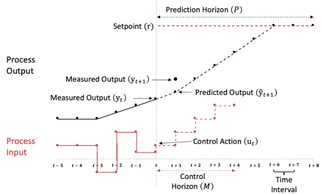
Figure 1. Model predictive control overview1 ... 8

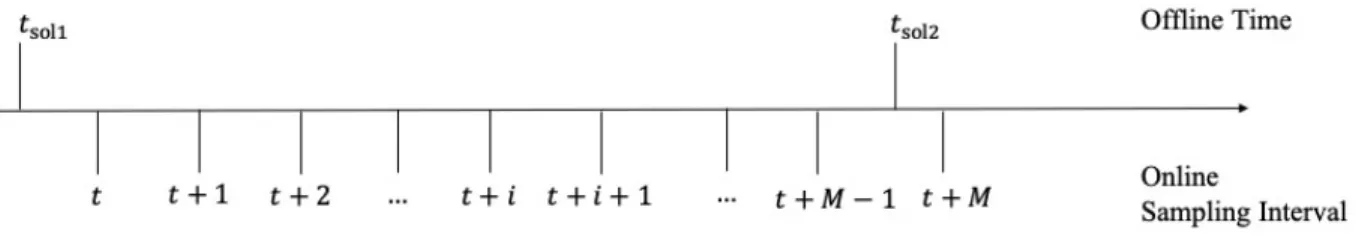
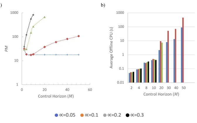
Figure 2. Key timepoints for the aro-MPC framework: 𝒕𝒔𝒐𝒍𝟏 and 𝒕𝒔𝒐𝒍𝟐, offline times for obtaining the explicit solution, 𝒕 and 𝒕 + 𝑴, the sampling intervals for implementing the first control law in the sequence, and 𝒕 + 𝑴 − 𝟏 the sampling interval for implementing the final control law in the sequence. 27 Figure 3. aro-MPC controller for Case Study 1 results for a range of control horizons and uncertainty set sizes: a) PM between the observed states and the setpoint, and b) average offline CPU (s) required to obtain the sequence of control laws. ... 33

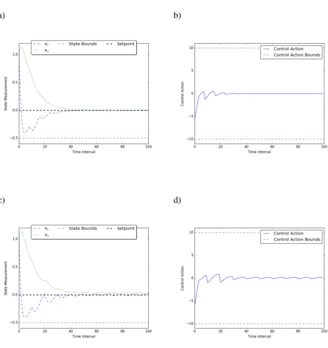
Figure 4. Case study 1: aro-MPC performance (∝= 0.1). a) state trajectory and b) control action profile (𝑀 = 8); c) state trajectory and d) control action profile (𝑀 = 10). ... 34

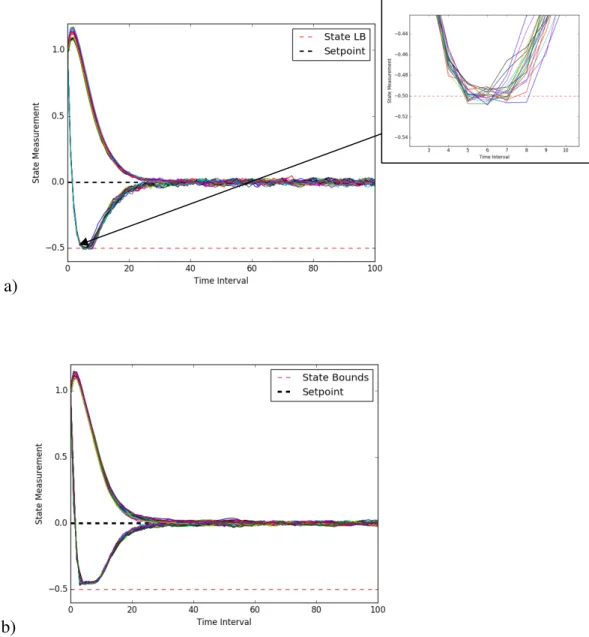
Figure 5. State trajectories for 20 random disturbance sequences. a) online MPC with 𝑴 = 𝟓𝟎, with focus on time intervals 3 to 10 to highlight time region where state violations occur, and b) aro-MPC with 𝑴 = 𝟓𝟎 and ∝= 𝟎. 𝟎𝟓. ... 38

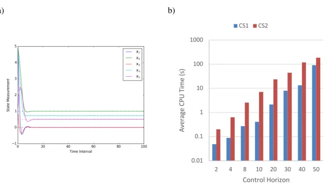
Figure 6. Case Study 2 (∝= 0.05). a) state trajectory over a 100-period time interval, and b) comparison of average CPU times for aro-MPC controllers of varying control horizons for Case Study 1 (CS1) and Case Study 2 (CS2). ... 41

Figure 7. State trajectories for 20 random disturbance sequences. a) online MPC with 𝑀 = 25, and b) aro-MPC with 𝑀 = 25 and ∝= 0.4. ... 44

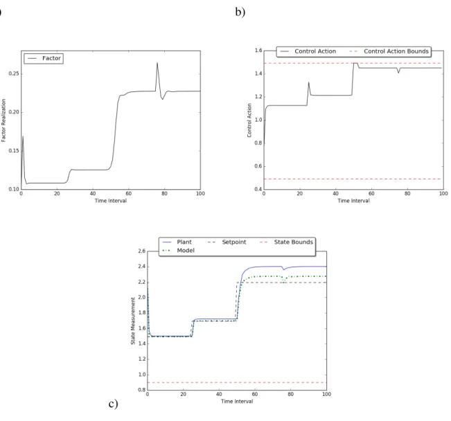
Figure 8. Case Study 3; a) factor realizations and disturbance sequence, b) control action sequence, and c) plant and model state trajectories as well as the user-defined setpoint. ... 45

Figure 9. Block flow diagram of the Sulfuric Acid plant. ... 48

Figure 10. Flowsheet for process gas (solid lines) and process acid (dashed lines). ... 51

Figure 11. Scrubbing tower flowsheet. ... 54

Figure 12. Steam utility flowsheet. ... 55

Figure 13. Cooling water utility flowsheet. ... 56

Figure 14. Changes in responding variables with respect to changes in the input variables. ... 70

Figure 15. Daily Profit and H2SO4 production rate near the optimal point at AF = 2,416 kg/hr, OBJ1 is shown in red and OBJ2 in green; the daily profit obtained at operating condition OP1 has also been included. The different colored trend lines are used to distinguish the gas strengths (GS) evaluated at different operating points. ... 75

Figure 16. Evaluation of the process constraints. The different colored trend lines are used to distinguish the gas strengths (GS) at different operating points. ... 76

(10)

Figure 17. Histogram for the two scenarios: minimum standard deviation (purple) and maximum expected value (green); also shown is the distribution at the operating condition OP1 (red). ... 80 Figure 18. Histogram for the SO2 concentration in the vent stream under uncertainty in the catalytic activity; also shown is the SO2 emission limit. ... 80

(11)

List of Tables

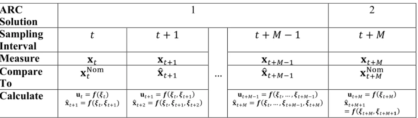
Table 1. Online implementation of the aro-MPC solution ... 28

Table 2. CPU time and PM for an aro-MPC with ∝= 𝟎. 𝟎𝟓 and 𝑴 = 𝟓𝟎 and an Online MPC with 𝑴 = 𝟓𝟎 subject to a variety of disturbance sequences over a 100-period time interval ... 36

Table 3. Nominal operating conditions for the main units in the Sulfuric Acid plant ... 48

Table 4. Model testing: Sulfuric Acid plant (percent error) ... 62

Table 5. Model validation ... 65

Table 6. Process variables considered in the sensitivity analysis ... 66

Table 7. Prices of raw materials and products ... 70

(12)

List of Abbreviations

ARO Adjustable robust optimization

aro-MPC Adjustable robust optimization model predictive control ARC Adjustable robust counterpart

AF Air Flow

CPU Central processing unit CO2 Carbon dioxide

CS1 Case study 1 CS2 Case study 2 DNA Data not applicable GA Genetic algorithm

GPS Generalized pattern search GS Gas Strength

H2S Hydrogen sulfide

H2SO4 Sulfuric acid

HX34T E-103 and E-104 Temperature HX5T E-105 Temperature

HX6T E-106 Temperature HX7T E-107 Temperature HX8T E-108 Temperature MPC Model predictive control

mp-MPC Multi-parametric model predictive control NaOH Sodium hydroxide

NRTL Non-random two-liquid model

O2 Oxygen

OBJ1 Objective 1 OBJ2 Objective 2

OP1 Operating Condition 1 OP2 Operating Condition 2 OPD Operating Condition Design

(13)

PEM Proton-exchange membrane pH E-24 Recirculation pH PK101 C-101 Height PK102 C-102 Height PK103 C-103 Height PK24 E-24 Height PK25 E-25 Height PM Performance metric SBS Sodium bisulfite Sc1 Scenario 1 Sc2 Scenario 2 Sc3 Scenario 3 Sc4 Scenario 4 SO2 Sulfur dioxide SO3 Sulfur Trioxide

(14)

List of Symbols

𝛉 Other model parameters captured in the explicit MPC solution ∆z9 Change in parameter z between sampling intervals 𝑖 and 𝑖 − 1 𝚽_𝟎 _{Bounded factor matrix relating primitive factors to}𝐱

𝚽₌ Bounded factor matrix relating primitive factors to 𝐞

𝝃 Uncertain primitive factors

ξ Set of parameters considered uncertain in the sulfuric acid optimization problem

𝝇 Definition of the uncertainty set

Ξ Set to which the primitive factors belong

𝛽 Bounded factor parameter

∝ Parameter used to adjust the size of the uncertainty set in aro-MPC 𝐀 State-space matrix that multiplies the states

𝐁 State-space matrix that multiplies the inputs 𝐂 State-space matrix that multiplies the outputs

𝐃 State-space matrix that multiplies the disturbances or errors

𝐝 Input disturbance

dV/d𝑡 Derivative of variable V with respect to variable 𝑡

𝐞 Uncertain additive time-varying error

𝐞M _{Lower bound on the uncertain additive time-varying error} 𝐞N _{Upper bound on the uncertain additive time-varying error}

𝐞𝐳 Vector of ones

𝒇 A general function

F Number of factors in the bounded factor uncertainty set FR Flowrate of the hot inlet stream

FS Flowrate of the cold inlet stream

𝐻 Enthalpy

𝑖 Number of sampling intervals into the future 𝑀̇_V Mass flowrate of component 𝑧

(15)

𝑃 Prediction horizon 𝐩M_{, 𝐩}N _{Dual variables} 𝑝_V Price of component 𝑧

𝐪 Objective cost associated with difference between process output and setpoint 𝑄`a==b Heat duty of the cooling tower E-110

ℝ Real number system

𝐫 Process setpoint

𝐫M_{, 𝐫}N _{Dual variables}

𝑡 Sampling interval

𝑡efg= Offline time for obtaining first aro-MPC solution 𝑡_efgh Offline time for obtaining second aro-MPC solution

𝐮 Control action

𝐮M _{Lower bound on control action} 𝐮N _{Upper bound on control action}

𝐔 Slope associated with linear decision rules for control actions 𝝊_lm9b _{Intercept associated with linear decision rules for control actions} 𝑣_op_q_{,elrstu hw} Volumetric concentration of SO2 in stream 24

V Volume in tank

𝐰 Objective cost associated with magnitude of control actions 𝑊za=b= Net work of the compressor B-101

𝐱 Process state

𝐱{ Predicted process state

𝐗 Slope associated with linear decision rules for process states 𝐱_l}~• _{Nominal state of the system at the sampling interval}_𝑡

𝐱M _{Lower bound on process state} 𝐱N _{Upper bound on process state}

𝝌_lm9b Intercept associated with linear decision rules for process states yM_{, y}N _{Dual variables}

𝐲 Process output

(16)

(17)

Chapter 1: Introduction

Chemical engineering systems are typically large, capital intensive projects, that operate over long periods of time. They can have large economic, environmental, and societal impacts on the regions in which they are situated. Thus, it is important that these systems be designed and operated in an optimal fashion. This thesis is composed of two distinct projects which address the issue of optimal operation of large chemical engineering systems.

In the first project a tool is developed to better enable the application of linear MPC to large systems under uncertainty. It is a framework for Explicit Linear Model Predictive Control (MPC). Linear MPC is considered an attractive strategy for achieving optimal control,1_{however its online}

computational requirements have typically restricted its application.2_{Explicit MPC circumvents}

this drawback by performing the expensive computation offline thereby reducing online computation to evaluation of a series of algebraic equations.3_{In this work, adjustable robust}

optimization (ARO) is used to develop an Explicit MPC framework.

The second study involves the simulation and economic optimization of an industrial-scale plant under uncertainty. This work is applicable when demand for the product being manufactured has increased and the operator wishes to identify the maximum profit or output that the plant can achieve given the current design and its associated safety, environmental and productivity restrictions. The use of simulation and optimization tools in this situation is highly advantageous as it can eliminate (or reduce) timely and costly experiments in search of the optimal operating condition. In this work, in collaboration with an industrial partner, a simulation was implemented, and a subsequent economic optimization was carried out to identify the optimal operating

(18)

condition for an industrial-scale sulfuric acid plant. Each of the research subjects mentioned above will be discussed next.

1.1Explicit MPC

MPC has largely been accepted as the solution for optimal control of complex multivariable processes.4_{The key idea in MPC is to compute the sequence of control actions that are expected}

to maintain the system on target by solving an optimization problem consisting of an internal process model, process constraints, and a user-defined objective function at each sampling interval. Only the first control action is implemented on the process and the procedure is repeated at the following sampling interval.4_{The primary issue raised by this procedure is that a large}

computational effort may be required to evaluate online an optimization problem thereby limiting its application to slowly varying processes.2_{However, this challenge can be overcome by solving}

offline the MPC optimization problem in a way that makes the relationship between the control actions and the measured outputs explicit.3_{This is referred to as}_{Explicit MPC}_{. The majority of}

work in the area of Explicit MPC has been accomplished using multi-parametric programming (mp-MPC).3_{Although it addresses the issue associated with online computation, the mp-MPC}

framework has its limitations. For instance, it is numerically difficult as it involves partitioning the state-space into polyhedral regions while avoiding overlaps in neighboring polyhedra.5_{Also, it}

does not guarantee that the state variables will remain within their feasible region under deterministic or uncertain conditions.6,7

1.2Modeling and Optimization of an Industrial-Scale Sulfuric Acid Plant

Sulfuric acid is an important industrial chemical because of its direct or indirect involvement in nearly all production industries. The main steps in the sulfuric acid manufacturing process are

(19)

combustion of sulfur into SO2, conversion of SO2 into SO3 in a multi-stage packed bed catalytic

reactor with inter-stage cooling, and absorption of SO3 in sulfuric acid. This is referred to as the

process gas cycle. An industrial sulfuric acid plant also consists of the process acid cycle, steam and cooling water utilities, and in some cases a scrubbing tower. Although this is a major industrial-scale application, the majority of modeling and optimization work in the literature aimed at sulfuric acid plants has focused solely on the catalytic reactor with very limited works integrating the complete process gas cycle. Moreover, there has only been two models that have been validated using actual plant data.8,9_{Finally, no studies have considered the effect of}

uncertainty in key model parameters on the economic performance and productivity of the sulfuric acid plant.

1.3Research Objectives

With respect to Explicit MPC, the aim of this work is to present a novel framework for obtaining the explicit solution to the linear MPC problem using adjustable robust optimization (ARO). This will be referred from heretofore as aro-MPC. Two objectives motivate this work: first, it is an alternative method to multi-parametric programming for obtaining the explicit solution to the linear MPC optimization problem; and second, the resulting framework is inherently robust with respect to the state variables, and thus guaranteed to satisfy process constraints without additional considerations. The novelty of this work, and its contribution to the area of optimal control, is the development of a new method for Explicit MPC. It is expected that the aro-MPC framework proposed here may broaden the applicability of Explicit MPC for controlling chemical engineering systems based on its differentiating features from mp-MPC.

(20)

In the second research subject, the objective is to develop a comprehensive model for an industrial-scale single absorption sulfuric acid plant with scrubbing tower that includes process utilities. By including the utilities and scrubbing tower, the model can account for more of the interactions between process variables, and thus will capture a more realistic representation of an actual industrial-scale plant. The model will be validated using historical data from an industrial-scale sulfuric acid plant, and thus it can be used to identify economic opportunities based on changes in the current operating conditions. Those opportunities will be identified deterministically and under uncertainty in key parameters to understand the sensitivity of the optimal operating condition and the price of robustness for the plant model. The comprehensive development of this steady-state model is expected to reduce the time and cost associated with identifying the optimal operating condition of the industrial-scale sulfuric acid plant. Moreover, it will enable an improved understanding of the interactions between operating parameters.

1.4Structure of Thesis

This thesis is organized as follows:

Chapter 2 provides a literature review highlighting the relevant works in the areas of Explicit MPC, ARO, and the design, simulation, and optimization of sulfuric acid plants.

Chapter 3 presents the proposed aro-MPC framework. Three notable computational experiments are included. The first uses a one input, two state system to demonstrate the general features of the framework. The second presents the aro-MPC for a 5x5 system. To the author’s knowledge, the largest system for which an Explicit MPC controller has been developed consists of three inputs and four outputs.10_{The third system demonstrates the implementation of the aro-MPC framework}

(21)

Chapter 4 describes the model used to approximate the industrial-scale sulfuric acid plant and the validation strategy. The model is then used to identify the optimal operating condition under deterministic and uncertain conditions. The content in this chapter has been published in Industrial & Engineering Chemistry Research.11_{This paper was written entirely by myself, and it was edited}

by my supervisor, Luis Ricardez-Sandoval. Permission has been granted by the publisher to use the published content in this thesis.

Chapter 5 summarizes the methods and results of this thesis and presents conclusions of both works. Recommendations are provided for future work in the areas of aro-MPC and simulation and optimization of industrial-scale sulfuric acid plants.

(22)

Chapter 2: Literature Review

This chapter provides detailed literature reviews on the most relevant contributions in the areas of Explicit MPC and ARO as well as the design, simulation, and optimization of sulfuric acid plants. Section 2.1 begins with a brief summary of linear MPC and is followed by a discussion on Explicit MPC and mp-MPC. Afterwards, an overview of ARO is presented. Section 2.2 presents the global importance of sulfuric acid by highlighting its most relevant applications. This is followed by a design overview of industrial-scale sulfuric acid plants and a presentation of the modeling works in the literature relevant to the production of sulfuric acid. A summary on the major findings and gaps identified from the literature review is presented at the end.

2.1Optimal Control Using MPC 2.1.1Linear MPC

As discussed in the introduction, MPC is an optimization-based control technique that employs a model of the system to compute the control actions that can minimize plant offsets. When compared to the conventional feedback control schemes such as PID control, MPC poses two key advantages; it can take into account process constraints, e.g. on the states and control actions of a system, and it can drive the controlled variables of the system in such a way that a user-defined objective is optimized.1_{More details about Model Predictive Control can be found elsewhere.}5,12

Linear MPC is typically defined by an optimization problem having linear constraints and a quadratic objective function, i.e.

(23)

min 𝐱{†‡ˆ∈ℝŠ‹, ∀9•=,…• 𝐮†‡ˆ∈ℝŠ•, ∀9•b,…•a= 𝐪‘_’(𝐲{ lm9− 𝐫lm9)h • 9•= + 𝐰‘ _{’ (∆𝐮} lm9)h •a= 9•= (1a) s. t. 𝐱{_lm9m== 𝐀𝐱{_lm9+ 𝐁𝐮_lm9 ∀𝑖 = 0, … , 𝑃 − 1 (1b) 𝐲{_lm9 = 𝐂𝐱{_lm9 ∀𝑖 = 0, … , 𝑃 (1c) 𝐮M _{≤ 𝐮} lm9 ≤ 𝐮N ∀𝑖 = 0, … , 𝑀 − 1 (1d) 𝐱M _{≤ 𝐱{} lm9≤ 𝐱N ∀𝑖 = 1, … , 𝑃 (1e) 𝐮_lm9 = 𝐮_lm•a= ∀𝑖 = 𝑀, … , 𝑃 − 1 (1f)

where 𝐱{_lm9 ∈ ℝ}‹_{is the vector of predicted states,}𝐲{_lm9 ∈ ℝ}™_{is the vector of predicted outputs,}

𝐮lm9 ∈ ℝ}• is the input control vector, 𝐫lm9 ∈ ℝ}™ is the vector of user-defined setpoints, and ∆𝐮lm9 ∈ ℝ}• is the vector containing the magnitude of the change in process inputs between time

interval 𝑡 + 𝑖 − 1 and 𝑡 + 𝑖 (i.e. ∆𝐮_lm9 = 𝐮_lm9− 𝐮_lm9a=). The initial condition is the measured output of the process at sampling time 𝑡, 𝐲_l∈ ℝ}™_{, which replaces}𝐲{

lm9at 𝑖 = 0. 𝑀 and 𝑃 are the

user-defined control and prediction horizons, respectively. Along with the weights on the controlled and manipulated variables (i.e. 𝐪 and 𝐰), 𝑀 and 𝑃 are the tuning parameters of the controller.

Linear MPC is implemented by solving online the MPC optimization problem (1a)-(1f). The general procedure is presented in Figure 1 for a single input single output system. At each time interval, 𝑡, the current output of the system y_l is measured and used as an initial condition to identify the sequence of control actions u_l, u_lm=, … , u_lm•a= that are expected to drive the future output predictions y_lm9 towards the user-defined setpoint subject to process constraints. Once solved, the first control action, u_l, is implemented on the process and the remaining are discarded.

(24)

Due to model limitations and plant-model mismatch, the predicted output, y{lm=, typically differs

from the measured output, ylm=. Hence, feedback is incorporated in the framework by repeating

the procedure at the following time interval.

Figure 1. Model predictive control overview1

2.1.2Explicit MPC using Multi-parametric Programming

In Explicit MPC, the MPC optimization problem is solved a priori to obtain explicit relationships between the control actions and measured outputs. The most general parametrization takes the following form:

(25)

such that function 𝒇is an algebraic function that is used to evaluate online the control actions 𝐮lm9

whichare dependent on the process state 𝐱lm9, the setpoint 𝐫 that was considered when obtaining

the parametric solution, and the remaining process model parameters 𝛉. The main feature of this approach is that the online computation of the control actions is reduced to evaluation of the function 𝒇 instead of solving an MPC optimization formulation at each sampling interval.

As mentioned in section 1.1, the majority of work in the field of Explicit MPC has been accomplished using mp-MPC. This approach involves partitioning the state-space into polyhedral regions such that for each region, an affine control law parametrized by the states of the system is obtained. In addition to evaluating the parametric control law, online implementation of the mp-MPC solution first involves selecting an appropriate control law by identifying the polyhedral region in which the current state measurement lies. Since the seminal work in this area showed the development of a mp-MPC controller for a constrained linear quadratic regulator,6_{the field}

has received much attention. Multiple studies have considered the topic of mp-MPC under uncertainty.2,13–16_{Uncertain optimization problems are solved using stochastic or robust}

optimization techniques.17–25_{In the former, the modeler must make an assumption regarding the}

probability distribution of the uncertain parameter whereas in the latter, no probability distribution is assumed, rather the uncertain parameter is defined by a bounded set. The robust solution is guaranteed to remain feasible over the entire range of uncertain parameter realizations whereas the stochastic solution only provides a probabilistic feasibility guarantee. Studies that have considered mp-MPC under uncertainty have obtained the robust explicit solution for systems with exogenous disturbances and/or model parameter uncertainty in the state-space matrices.2,13,14_{The area of}

Explicit Stochastic MPC has recently been referred to as an important area of future work.27_With

(26)

and medical sectors through the control of a PEM fuel cell and an intravenous anaesthesia system, respectively.10,28_{Other chemical engineering applications that have been considered include}

control of distillation columns and pressure swing absorption systems.29,30_{All of the previous}

works mentioned have developed the mp-MPC for systems with linear process models; however there has also been a few studies that have developed the mp-MPC for systems described by nonlinear models.31–33_{The main limitation of mp-MPC is the numerical difficulty associated with}

computing every polyhedron in the state-space while avoiding overlaps and gaps in neighbouring polyhedra.5_{To the author’s knowledge, the largest system to which mp-MPC has been successfully}

applied is the three input, four state PEM fuel cell system.10_{In addition to eliminating the drawback}

associated with online computation, another advantage of the robust mp-MPC controllers is that they ensure controller feasibility against a user-defined uncertainty set. However, to the author’s knowledge, they do not guarantee that the state-space variables will remain within a feasible region in the presence of uncertainty. Although some works have been aimed at reducing the computational complexity associated with solving the mp-MPC optimization problem through the identification of suboptimal solutions using a variety of approximation techniques,34–40_{there has}

been limited contributions that explore alternative methods of obtaining explicit functions (1) for linear MPC. However, there has been some works that explore the use of machine learning methods to obtain the explicit functions (1) for nonlinear MPC.41,42_{A technique that will be}

considered in this study to address uncertainty in the Explicit MPC formulation developed in this work is presented next.

2.1.3Adjustable Robust Optimization

(27)

(immune) against a user-defined uncertainty set but the user is unable to incorporate any information that becomes available after the optimization problem is solved without performing re-optimization. ARO has the same advantage of SRO in that the resulting solution is robust against a user-defined uncertainty set; however, the user can select “wait-and-see” decision variables to be adjustable in the ARO framework. In a conventional ARO problem, those variables selected as adjustable are replaced by a user-defined function where the independent variables (i.e. inputs to those functions) are the uncertain parameters. Hence, the coefficients of these functions replace the original variables as the decision variables in the ARO formulation. The resulting expressions are then used to evaluate the adjustable (manipulated) variables at a later point in time when the uncertain parameters have materialized (been observed).

The optimization problem considered to obtain the ARO solution is a deterministic reformulation of the robust multistage optimization problem.43_{This problem is referred to as the adjustable robust}

counterpart (ARC). For linear optimization problems, it consists of replacing all adjustable variables with their corresponding parametrized functions of the uncertain parameters followed by elimination of the uncertain parameters from all uncertain constraints including the objective function. This is performed by dualization for inequalities constraints and by coefficient matching for equality constraints.

ARO has been applied in the area of process scheduling to develop two-stage and multi-stage robust schedules for batch processing plants.44–47_{With regards to process control, it has been}

shown that ARO can be used to obtain time-varying control laws for fully linear control problems (i.e. linear objective function and linear constraints) by parametrizing the control action with the measured disturbances rather than the measured states as is done in the multi-parametric programming framework.26,48_{However, online implementation of the control laws is not discussed}

(28)

beyond stating that the laws are to be implemented in a time-varying fashion nor is their performance evaluated. Although those works focus on the design of optimal linear controllers, they represent the closest attempt to obtaining an explicit solution of the linear MPC problem with a quadratic objective function using ARO.

2.2Sulfuric Acid Manufacturing Process and Simulation

The most dominant application of sulfuric acid is in the production of phosphate fertilizers, accounting for almost 60% of global consumption in 2009.49_{Other applications include leaching}

of copper, nickel, and uranium ores, petroleum refining to convert low molecular weight alkenes to alkylates, manufacturing of rubber, plastics, pigments, pulp and paper, and the production of other chemicals and fertilizers.49_{In addition to its application in multiple industries, a secondary}

benefit of sulfuric acid is that it is mainly produced involuntarily for the purpose of mitigating SO2

and H2S.50 These gases are produced during the processing of metal ores and hydrocarbons,

respectively, and are the sources of sulfur for sulfuric acid production. The sulfuric acid production process, also known as the contact process, can directly make use of the SO2 but H2S must first be

converted into elemental sulfur. Globally, 60% of sulfur used in the production of sulfuric acid comes from hydrocarbons, 30% from metal ores, and the remaining 10% from the decomposition of spent petroleum and polymer sulfuric acid catalyst.51

There are two types of manufacturing plants: single and double adsorption. Double absorption plants can operate at SO2 concentrations as high as 12% and can achieve SO2 conversion as high

as 99.6% whereas single absorption plants can have SO2 concentrations up to 10% while achieving

SO2 conversion as high as 98.5%.52 Furthermore, the resulting process gas from a double

(29)

required to reduce the concentration of SO2 in the vent gas from a single absorption column to

environmentally acceptable levels.53_{This can be attributed to the inter-stage absorption column}

that is included between the third and fourth reactor stages for double absorption plants.54

However, with the aid of the scrubbing unit, single absorption plants produce a vent gas with a concentration lower than 100 ppm SO2 whereas the double absorption plants produce a vent gas

with a concentration of 400-450 ppm SO2.53 Moreover, the scrubbing tower makes operation

during transient periods such as plant start up significantly easier. While the temperature in the packed beds of the reactor is increasing to the catalyst activation temperature, unreacted SO2 in

the process gas is still being removed so that a vent gas which meets environmental standards is produced.53,55_{For these reasons, single absorption sulfuric acid plants continue to be viable}

alternatives to the more productive double absorption plants.56

Despite its importance, the majority of the theoretical work reported in the literature for this process has been very limited and focused only on modeling the reactor section of the contact process. To the author’s knowledge, only one reactor model has been validated using industrial plant data. In that work, a transient model of a multi-stage reactor was created in DYNAM to minimize SO2 emissions during plant start-up.8 That work was later extended to include transients

during operation when SO2 concentration in the vent gas from the metallurgical plant may

fluctuate.57_{Moreover, other studies have considered the use of alternative reactors, mainly}

trickle-bed and periodic flow reversal reactors, which eliminate the need for inter-stage cooling. In those works, mechanistic models of the reactors were developed. Those models were validated by comparison with experimental lab data and thereby established the relationships between the design, operating parameters and reactor performance.58–61_{Furthermore, there have been reports}

(30)

operation of the multi-stage reactor through a reduction in entropy,62_{re-distribution of the catalyst}

throughout the different stages,63_{and real-time set-point calculation of the first stage inlet}

temperature for process gas with a fluctuating concentration of SO2.64

To the author’s knowledge, there has only been very limited modeling studies in the literature which attempt to model other sections of the contact sulfuric acid plant, in addition to the reactor section. In one of those studies, a single absorption sulfuric acid plant using metallurgical ore roaster gas as the source of SO2 was simulated at steady state using PROPS.9 The simulation

included the process gas and process acid cycles. To validate the simulation, temperature results from the multiple reactor stages and overall conversion from the model were compared to real plant data. An economic optimization was performed for the plant and it was found that a 0.32% increase in return on investment was possible at the optimal solution. This translated into an annual net earnings increase of $40,000. In that study, the decision variables being considered were the inter-stage heat exchanger outlet temperatures and catalyst loadings in the multiple reactor stages. In another study, a transient model of a double absorption sulfuric acid plant that uses elemental sulfur as the feedstock was completed using gProms.65_{That model also included the complete}

process gas cycle; however, the process acid cycle only presented the acid streams in the absorption columns. That study suggested that potential SO2 emissions reductions of up to 40% were possible

by optimizing feed flow rates and split fractions. Although there have been studies that aim to minimize the SO2 emissions from the sulfuric acid plant and maximize its economic performance,

there has not been a study that provides insight on the sensitivity of the economic performance of a sulfuric acid plant with respect to the operating conditions. Also, the effect of uncertainty in key model and optimization parameters on economic performance has not been previously considered

(31)

for this plant. Furthermore, the cooling water utility and scrubbing tower have not been included in the models reported in the literature.

2.3Summary

Explicit MPC is an attractive alternative to solving the linear MPC optimization problem online as it significantly reduces the online computational burden. It results in control laws that are parametrized by the measured states of the system and which are evaluated when the process is online. Many works have explored this topic using multi-parametric programming (mp-MPC). Studies in mp-MPC have explored the topics of MPC under uncertainty, MPC for real-world systems such as fuel cells and pressure-swing absorption columns, MPC for nonlinear systems, and approximate explicit solutions to the linear MPC optimization problem. The final topic in the previous list addresses one of the main drawbacks associated with mp-MPC. Namely, the complexity associated with identifying the explicit control laws as a result of the need to partition the state-space while avoiding partition overlaps. Secondly, although mp-MPC under uncertainty has been considered, the resulting control laws have not been shown to be robust with regards to the states of the system. ARO, a method for obtaining robust solutions to uncertain multi-stage optimization problems, is considered a suitable alternative to multi-parametric programming for obtaining the explicit solution to the linear MPC optimization problem. Its benefits are that it is an inherently robust technique and it does not require partitioning the state-space. Within chemical engineering it has mainly been applied to the area of process scheduling. The following chapter presents the proposed framework for aro-MPC.

Sulfuric acid is an important global commodity due to its use in many production processes and its ability to mitigate SO2 and H2S. Although the sulfuric acid plant can consist of up to five process

(32)

cycles (process gas, process acid, steam utility, cooling water utility, and scrubbing tower) the majority of modeling works in the literature have focused on modeling the catalytic reactor. Of the limited works that develop more comprehensive models by incorporating other major process units, none have developed a complete sulfuric acid plant model. Moreover, the effect of uncertainty in key operating parameters on the plant performance has not been considered. Thus, there is great motivation for developing a comprehensive model that includes all components of the industrial-scale sulfuric acid plant, including its utilities, to explore the economic and environmental benefits of alternative operating conditions. This topic is addressed fully in chapter 4.

(33)

Chapter 3: Design of an Explicit Model Predictive Controller using ARO

In this chapter the proposed framework for Explicit MPC using ARO is presented. It begins with the reformulation of the deterministic linear MPC optimization problem presented in Section 2.1.1 into the robust problem that is considered in this work. Afterwards, a detailed description of ARO is provided and is followed by the development of the aro-MPC framework and a comparison to mp-MPC. Finally, computational experiments consisting of three case studies are presented to demonstrate the features of the proposed framework.

3.1Robust State-Space Model for Linear MPC

The present research work considers only those systems having all states as measurable variables, i.e. 𝐂 ∈ ℝ}‹›}‹_{is an identity matrix. Thus, equation (1c) is not presented in future model} formulations to simplify the analysis. Moreover, the following model subject to uncertainty (i.e. robust model) is considered:

𝐱{_lm9m== 𝐀𝐱{_lm9+ 𝐁𝐮_lm9+ 𝐃𝐞_lm9m= ∀𝑖 = 0, … , 𝑃 − 1 (3)

where 𝐞_lm9 ∈ ℝ}œ_{is the vector of uncertain additive time-varying errors between the model and} the actual plant, i.e. 𝐞_lm9 = 𝐱_lm9− 𝐱{_lm9. Thus, equation (3) replaces equation (1b).

In an online MPC implementation, the newly introduced term above 𝐞 is more commonly recognized as a measurable input disturbance 𝐝. In the present explicit aro-MPC framework 𝐞 is used to capture all sources of error between the state prediction and actual state measurement. This capability has been demonstrated previously in the literature where the additive error was used to represent a variety of modelling uncertainties including nonlinearities and hidden dynamics.66,67

(34)

laws), 𝐞lm9 is assumed to belong to a convex polyhedral set, i.e. 𝐞M ≤ 𝐞lm9 ≤ 𝐞N. Thus, the modeler

is able to estimate a priori the bounds on the error between the state predictions obtained from the process model and those measured from the actual plant. When the explicit solution is being implemented online, 𝐞lm9 is assumed to be zero in the sampling interval 𝑡 + 𝑖 − 1 when predicting 𝐱{_lm9 and its actual realization is evaluated in the sampling interval 𝑡 + 𝑖 upon observing the actual state of the system 𝐱_lm9. This is discussed in further detail in section 3.2.3.

Unlike the typical state-space representation of the input disturbance, which has the same time index as 𝐮(i.e. 𝐱{_lm9m== 𝐀𝐱{_lm9+ 𝐁𝐮_lm9+ 𝐃𝐝_lm9), here the time index for the uncertain additive error is the same as the state being predicted, as shown in equation (3). This is done to guarantee that the state predictions of the present aro-MPC formulation are robust estimates for the actual measured states of the process.

Whereas it would act as an initial condition in the online MPC framework, the state of the system

𝐱_l in the present aro-MPC framework will not be observed prior to resolving the problem given that the optimization is being completed offline. Hence, 𝐱l is also considered as an uncertain

(unknown) parameter at the time of solving the explicit aro-MPC problem offline and is assumed to belong to a convex polyhedral uncertainty set: 𝐱M _{≤ 𝐱}

l≤ 𝐱N.

Equations (1) and (3) with the exception of (1b) are referred to as the robust linear MPC optimization problem. The following section develops the aro-MPC framework out of the robust

(35)

linear MPC optimization problem and presents a control policy for online implementation of the explicit solution.

3.2Framework for Linear Explicit MPC using ARO (aro-MPC)

This section begins with a general overview of ARO and its use in solving uncertain multistage optimization problems. Afterwards, the necessary components for solving the robust linear MPC optimization problem using ARO are presented and they are used to develop the adjustable robust counterpart (ARC), which is a necessary step in the ARO formulation. The procedure for implementing the aro-MPC framework is discussed at the end of this section.

3.2.1Handling Uncertainty in Linear MPC

There are three approaches to handling uncertainty in MPC.4,5_{The first involves ignoring the}

uncertainty in the closed loop nominal MPC and accepting its inherent, but limited, robustness. In the second approach referred to as open loop min-max MPC, uncertainty is taken into consideration by identifying a sequence of control actions for a known initial state and uncertainty set such that the states will remain feasible for any disturbance sequence that materializes. In the last approach, feedback min-max MPC considers the system as a closed loop subject to realizations of the uncertain parameter and optimization occurs over a sequence of control laws rather than control actions. In pursuing the latter approach, the robust linear MPC optimization problem can be considered as a multistage optimization problem. In this work, adjustable robust optimization (ARO) is used to obtain the feedback min-max MPC solution offline. As with the change from open loop to feedback min-max MPC,4_{searching for the robust solution using ARO as opposed to}

(36)

3.2.2Developing the ARC for the Robust Linear MPC Optimization Problem

As it applies to the robust linear MPC optimization problem the key decisions that the modeler must make to solve the problem using ARO are:

• Identify the uncertain parameters and their corresponding uncertainty set.

• Define the parametric representation for the “wait-and-see” decision variables.

As mentioned above, the parameters in the uncertain linear MPC optimization problem being considered as uncertain are the initial state of the system 𝐱_l and the additive time-varying uncertain error 𝐞_lm9. Those uncertain parameters are recast as functions of primitive uncertain parameters

𝝃_lm9 ∈ ℝ•ž_{referred to as factors. The formal definitions for the factor representations of the} original uncertain parameters are as follows:

𝐱_l = 𝐱_l}~•_{+ 𝚽}

𝟎𝝃l (4)

𝐞_lm9 = 𝚽₌𝝃_lm9 ∀𝑖 = 1, … , 𝑃 (5)

where 𝐱_l}~• _{∈ ℝ}}‹ _{is the vector of expected values for the states of the process in the first} sampling interval, whereas matrices 𝚽_b ∈ ℝ}‹×}ž _and 𝚽

= ∈ ℝ}œ×}ž contain user-defined

constants relating the primitive factors to the uncertain parameters.

The uncertain factors 𝝃 are assumed to be represented by a bounded factor model. This definition of the uncertainty set has two attractive features when considering application of the framework proposed here to large, real-world systems. Firstly, the factors can capture non-trivial parameter correlations that can readily be identified from historical data.68_{Secondly, the uncertainty set is}

(37)

polyhedral; thus, it can be easily accommodated into linear ARO. The description of the uncertainty set is as follows:

𝝇= ⎩ ⎪ ⎨ ⎪

⎧ ¤𝐱𝑡 ∈ ℝNx: 𝐱𝑡 = 𝐱𝑡Nom+ 𝚽0𝝃𝑡 for some 𝝃𝑡 ∈ Ξ𝑡; 𝐱L ≤ 𝐱𝑡 ≤ 𝐱U®

¤𝐞𝑡+𝑖 ∈ ℝNe: 𝐞𝑡+𝑖 = 𝚽1𝝃𝑡+𝑖 for some 𝝃𝑡+𝑖 ∈ Ξ𝑡+𝑖; 𝐞L ≤ 𝐞𝑡+𝑖 ≤ 𝐞U® ∀𝑖 = 1, … , 𝑃

where Ξ𝑡+𝑖 is defined as:

Ξ𝑡+𝑖 =¤𝝃𝑡+𝑖 ∈ ℝNF: 𝝃𝑡+𝑖 ∈[−𝐞𝐳, +𝐞𝐳], 𝐞𝐳T𝝃𝑡+𝑖 ∈[−𝛽F, +𝛽F], 𝛽 ∈[0,1]® ∀𝑖 = 0, … , 𝑃⎭

⎪ ⎬ ⎪ ⎫ (6)

where 𝐞𝐳 ∈ ℝ}ž_{denotes the vector of ones,}F_{is the number of factors, and the scalar}𝛽_{is a user} defined constant in addition to the previously introduced matrices 𝚽_b and𝚽₌. Thus, the range of the individual primitive factors is limited to |1| and additional information regarding their interdependencies can be used to further reduce their range by reducing the value of 𝛽, as shown in (6). Note that the convex polyhedral bounds for 𝐱_l and 𝐞_lm9 introduced in section 3.1 have also been explicitly included in the uncertainty set description (6). A description of how the uncertainty set is defined is presented in Section 3.3.1.

The control actions are the primary decision variables of interest to be adjustable to the uncertain time-varying error 𝐞. However, to maintain equality of the constraints (3) when adjusting the control action based on different realizations of the uncertain parameters, it is necessary to also define the predicted process states as adjustable variables. Several alternative representations for the parametrized function have been proposed by various researchers when developing an ARO framework.69–71_{Affine relationships are often considered in the interest of numerical tractability.}26

(38)

follows: 𝐮_lm9 ← 𝝊_lm9b _{+ ’ 𝐔} lm9,º𝝃º lm•a= º•l ∀𝑖 = 0, … , 𝑃 − 1 (7) 𝐱{_lm9 ← 𝝌_lm9b _{+ ’ 𝐗} lm9,º𝝃º lm• º•l ∀𝑖 = 1, … , 𝑃 (8)

where the vectors 𝝊_lm9b _{∈ ℝ}}•_and𝝌

lm9

b _{∈ ℝ}}‹_{represent the intercepts whereas the elements in the} matrices 𝐔_lm9 ∈ ℝ}•×}ž_and 𝐗

lm9 ∈ ℝ}‹×}ž represent the slopes of the respective affine

expressions. Thus, the variables 𝝊_lm9b _and_𝐔

lm9 as well as 𝝌lm9b and 𝐗lm9 replace the original

variables 𝐮_lm9 and 𝐱{_lm9, respectively, as the decision variables of the robust MPC optimization problem.

To reduce the conservativeness of the control laws, full recourse is considered in the aro-MPC framework. That is, the adjustable variables are not restricted to be functions of the most recent realizations of the uncertain parameters but rather are allowed to be a function of all previously observed values of uncertainty. Thus, the control action 𝐮_lm9 and the predicted process state 𝐱{_lm9

are both defined as explicit functions of the primitive factors 𝝃l, … , 𝝃lm9. This is reflected in the

present framework by including the following non-anticipativity restrictions:

𝐔_9º = 𝟎 ∀𝑗 > 𝑖 (9)

(39)

this work, the ARO method is adapted for the aro-MPC framework so that the first control actions can be computed as affine functions of the first observed state of the process, xt. Note that the

mp-MPC framework is the same in that all control actions are evaluated using measured states of the process. In the present aro-MPC formulation, this is accomplished by solving all of the original decision variables (𝐮_lm9 ∀𝑖 = 0, … 𝑃 − 1, 𝐱{_lm9 ∀𝑖 = 1, … 𝑃) as adjustable variables, and thus having no “here-and-now” decisions.

3.2.2.1Formulating ARC

For the robust linear MPC optimization problem defined by equations (1) and (3), excluding (1b), the full ARC is formulated by replacing the adjustable variables with their affine

expressions, equations (7) and (8), considering the non-anticipativity restrictions, equations (9) and (10), and incorporating the uncertainty set description (6) to reformulate the uncertain equality and inequality constraints by coefficient matching and dualization, respectively. Note that the adjustable variables in the objective function are only replaced by their respective intercepts and not the complete affine functions. Hence, the resulting solution is robust in its satisfaction of the process constraints, but the objective function is reflective of the expected

(40)

rather than the worst-case realization of the uncertain parameters. This was done to avoid the need to dualize the nonlinear objective function which is left for future studies.

Based on the above, the following is the ARC for the equality constraint (3) after coefficient matching: 𝝌_lm=b _{= 𝐀𝐱} l }~•_{+ 𝐁𝝊} l b _(11a) 𝐗_lm=,l = 𝐀𝚽_𝟎+ 𝐁𝐔_l,l (11b) 𝝌_lm9m=b _{= 𝐀𝝌} lm9 b _{+ 𝐁𝝊} lm9 b _{∀𝑖 = 1, … , 𝑃 − 1} _(11c) 𝐗_lm9m=,º = 𝐀𝐗_lm9,º+ 𝐁𝐔_lm9,º ∀𝑗 = 𝑡, … , 𝑡 + 𝑖 ∀𝑖 = 1, … , 𝑃 − 1 (11d) 𝐗_lm9m=,lm9m= = 𝐃𝚽₌ ∀𝑖 = 0, … , 𝑃 − 1 (11e)

Similarly, the following is the ARC for each row 𝑛 = 1, … , N› of the lower bound of the uncertain

(41)

’ 𝐞𝐳_¾‘_𝐩 lm9,¿,º N ₊ lm9 º•l ’ 𝐞𝐳_¾‘_𝐩 lm9,¿,º M ₊ lm9 º•l ’ 𝛽Fy_lm9,¿,ºN lm9 º•l + ’ 𝛽Fy_lm9,¿,ºM lm9 º•l + À𝐱N_{− 𝐱} l }~•_Á𝐫 lm9,¿,lN + À𝐱_l}~•_{− 𝒙}M_Á𝐫 lm9,¿,lM + ’ 𝐞N_𝐫 lm9,¿,ºN lm9 º•lm= + ’ 𝐞M_𝐫 lm9,¿,ºM lm9 º•lm= ≤ 𝒙_lm9(¿)b _{− 𝐱} (¿) M ∀𝑖 = 1, … , 𝑃 (12a) 𝐩_lm9,¿,lN _{− 𝐩} lm9,¿,l M _{+ y} lm9,¿,lN 𝐞𝐳¾ − ylm9,¿,lM 𝐞𝐳¾ + 𝚽_b‘_𝐫 lm9,¿,lN − 𝚽b‘𝐫lm9,¿,lM = −𝐗lm9,l(¿)‘ ∀𝑖 = 1, … , 𝑃 (12b) 𝐩_lm9,¿,ºN − 𝐩_lm9,¿,ºM + y_lm9,¿,ºN 𝐞𝐳Ã− ylm9,¿,ºM 𝐞𝐳Ã + 𝚽₌‘_𝐫 lm9,¿,ºN − 𝚽=‘𝐫lm9,¿,ºM = −𝐗lm9,º(¿)‘ ∀𝑗 = 𝑡 + 1, … , 𝑡 + 𝑖 ∀𝑖 = 1, … , 𝑃 (12c) 𝐩_lm9,¿,ºN _{, 𝐩} lm9,¿,º M _{, 𝐫} lm9,¿,ºN , 𝐫lm9,¿,ºM ≥ 𝟎 ∀𝑗 = 𝑡, … , 𝑡 + 𝑖 ∀𝑖 = 1, … , 𝑃 (12d) y_lm9,¿,ºN _{, y} lm9,¿,º N _{≥ 0} _{∀𝑗 = 𝑡, … , 𝑡 + 𝑖} ∀𝑖 = 1, … , 𝑃 (12e) where 𝐩_lm9,¿,ºN _,_𝐩 lm9,¿,º M _{∈ ℝ}}ž_,𝐫 lm9,¿,ºN , 𝐫lm9,¿,ºM ∈ ℝ}™, and ylm9,¿,ºN , ylm9,¿,ºM ∈ ℝ, ∀𝑛 = 1, … , N›, ∀𝑗 = 𝑡, … , 𝑡 + 𝑖, ∀𝑖 = 1, … , 𝑃. In equations (12a) to (12e), 𝐚_(¿) and 𝐀_(¿) are general representations used to denote the nth_{element of vector}_𝐚_{(a scalar) and the n}th_{row of a matrix}_𝐀

(a row vector), respectively. The complete ARC for the robust linear MPC optimization problem can be found in Appendix A. For a complete description on formulating the ARC the reader is referred to other sources.47

3.2.3aro-MPC Framework Implementation

(42)

is solved offline. In this work, the optimization solver IPOPT was used to identify the optimal solution. Note that the process is assumed to be in continuous operation. Thus, the state of the system is not explicitly considered at the time of solving the ARC to obtain the explicit control laws. Rather, any known state of the system at the time of solving the ARC is only implicitly considered since it is used as an estimate for 𝐱_l}~•_{. The inputs to solve the ARC are}_𝐱

l

}~•_{, the}

typical information required to solve the deterministic optimization problem defined by equations (1) with the exception of the initial state of the system, i.e. 𝑀, 𝑃, 𝐪, 𝐰, 𝐀, 𝐁, 𝐂, and𝐃, and a fully defined uncertainty set 𝝇, as shown in (6).

A timeline for solving offline the full ARC and implementing the explicit solution is presented in Figure 2. The sampling interval in which the first control law of the explicit solution is to be implemented is defined as 𝑡. The modeler must begin solving the ARC at an offline time 𝑡Æ~Ç=

where the requirement is that the difference between 𝑡_Æ~Ç= and 𝑡 be greater than or equal to the time required to solve the ARC. At 𝑡_Æ~Ç= an estimate of 𝐱_l}~•_{is required. The estimate can be obtained}

using the current state of the system. The number of affine expressions obtained as control laws, equations (7), is the same as the control horizon (𝑀) defined by the modeler. Moreover, the control laws are implemented in sequence in a time-varying manner. Thus, at sampling interval 𝑡 + 𝑀 − 1 the final control law is implemented and another explicit solution is required to continue controlling the process at sampling interval 𝑡 + 𝑀. Therefore, the ARC must be solved once again

(43)

at an offline time 𝑡Æ~Çh before 𝑡 + 𝑀, as shown in Figure 2.

Figure 2. Key timepoints for the aro-MPC framework: 𝒕_{𝒔𝒐𝒍𝟏} and 𝒕_{𝒔𝒐𝒍𝟐}, offline times for obtaining the

explicit solution, 𝒕 and 𝒕 + 𝑴, the sampling intervals for implementing the first control law in the sequence, and 𝒕 + 𝑴 − 𝟏 the sampling interval for implementing the final control law in the sequence.

The online implementation of the resulting control laws is presented in Table 1. It is assumed that the control laws for time interval 𝑡 to 𝑡 + 𝑀 − 1 are available by solving the full ARC formulation at 𝑡Æ~Ç=, referred to as ARC Solution 1. Thus, at the sampling interval 𝑡 the state of the system 𝐱l

is measured and compared to the expected state 𝐱_l}~•_{to obtain the factor realization}_𝝃

l using

equations (4). The control action 𝐮_l and the predicted state of the system 𝐱{_lm= are calculated using their respective affine functions, equations (7) and (8), as obtained in ARC Solution 1. For the latter, 𝝃_lm= is assumed to be 0 as it has not yet materialized. 𝐱{_lm= can be seen to be a function of

𝝃_lm= as per equation (11e) where the slope 𝐗_lm9m=,lm9m= has not been eliminated by the non-anticipativity restriction, equation (10).This occurs as a result of the uncertain time-varying error having the same time index as the state being predicted in the original robust model as shown in equation (3). The procedure for the sampling intervals 𝑡 + 1 to 𝑡 + 𝑀 − 1 is the same with the exception that comparison of the actual and predicted states of the system, 𝐱_lm9 and 𝐱{_lm9, respectively, is performed using equations (5) instead of (4). As discussed in Section 3.2.2, full recourse is considered in the present aro-MPC framework. Thus, the control law is a function of

(44)

all uncertain parameters materializing, starting from the first sampling interval in which the current ARC Solution was applied. Before the systems reaches 𝑡 + 𝑀, a second ARC formulation needs to be resolved at time tsol2 (referred to as ARC Solution 2). Accordingly, when implementing ARC

Solution 2 in sampling interval 𝑡 + 𝑀, the first control law in the sequence is only a function of the uncertain factor 𝝃lm•, as shown in Table 1.

Table 1. Online implementation of the aro-MPC solution

ARC Solution 1 2 Sampling Interval 𝑡 𝑡 + 1 … 𝑡 + 𝑀 − 1 𝑡 + 𝑀 Measure 𝐱_l 𝐱_lm= 𝐱_lm•a= 𝐱_lm• Compare To 𝐱l }~• _𝐱{ lm= 𝐱{lm•a= 𝐱lm•}~• Calculate 𝐮l= 𝒇(𝝃l) 𝐱{lm== 𝒇(𝝃l, 𝝃lm=) 𝐮lm== 𝒇(𝝃l, 𝝃lm=) 𝐱{lmh= 𝒇(𝝃l, 𝝃lm=, 𝝃lmh) 𝐮lm•a== 𝒇(𝝃l, … , 𝝃lm•a=) 𝐱{lm•= 𝒇(𝝃l, … , 𝝃lm•a=, 𝝃lm•) 𝐮lm•= 𝒇(𝝃lm•) 𝐱{lm•m= = 𝒇(𝝃lm•, 𝝃lm•m𝟏)

A novel feature of the present aro-MPC framework is that it is guaranteed to remain feasible for any sequence of uncertain parameters of length 𝑀 belonging to the pre-defined uncertainty set 𝝇. Thus, the calculated control laws are such that the observed states of the system over the control horizon 𝑀 will remain within their bounds, equations (1d). This is a direct consequence of the ARO method and the resulting decision rules for adjustable variables being fully robust for realizations of the uncertain parameter within the user-defined uncertainty set.26

3.2.4Comparison to mp-MPC

Although the mp-MPC and aro-MPC frameworks yield explicit feedback control laws to the linear MPC optimization problem, there are some key differences between the two approaches. The main advantage of the mp-MPC framework is the optimization problem does not have to be resolved for a new explicit solution after an elapsed number of time intervals. Both the aro-MPC and

(45)

mp-MPC frameworks require re-optimization if the setpoints of the system change or the modeller wishes to update the uncertainty set. However, to guarantee feasibility, the time-varying nature of the aro-MPC controls laws results in required re-optimization when the sequence of control laws is exhausted, even if the system is at steady-state. In addition to not having to partition the state-space into polyhedral regions, another advantage of the present aro-MPC framework is that controller feasibility is guaranteed, i.e. when evaluated, the control laws are guaranteed to maintain the states of the system within their feasible region for any sequence of uncertain parameters materializing within the user-defined uncertainty set.

3.3Results

This section presents three case studies that demonstrate the capabilities of the proposed aro-MPC framework. The first case study highlights the effects of the size of the uncertainty set and the length of the control horizon on the CPU time required to obtain the control laws and the resulting controller performance. This is followed by a comparison to online MPC for four disturbance sequences. The second case study considers a 5x5 system to highlight the applicability of the framework to larger systems. In the final case study a linear model is used to approximate a nonlinear plant to demonstrate that the uncertain additive time-varying error can capture error resulting from plant-model mismatch.

3.3.1 Case Study 1

The following single input two state system has been adapted from the seminal work on mp-MPC:6

𝐱_lm9m== È0.7326 −0.0861

0.1722 0.9909 Í 𝐱lm9+ È0.06090.0064Í ulm9+ È0.1 0

(46)

𝐱_lm9≥ −0.5 _{∀𝑖 ≥ 0} (13b)

−10 ≤ ulm9 ≤ 10 ∀𝑖 ≥ 0 (13c)

È−0.11_−0.11Í ≤ 𝐝lm9≤ È0.11_0.11Í ∀𝑖 ≥ 0 (13d)

The aro-MPC solution is obtained for the above system under the assumption that the plant defined by equations (13a) can be perfectly modeled with the exception of the unmeasurable disturbance

d. Thus, the following equations are used as a robust model for the plant equations (13a):

𝐱{_lm9m== È0.7326 −0.0861_0.1722 _0.9909 Í 𝐱{_lm9+ È0.0609_0.0064Í u_lm9+ È1 0_{0 1}Í 𝐞_lm9m= ∀𝑖 = 0, … , 𝑃 − 1 (14)

As in the original mp-MPC work, the objective is to regulate the system to the origin. The robust linear MPC optimization problem for this system has the following objective function:

𝑃𝑀 = ’Àx{_=,lm9h _{+ x{} h,lm9h Á • 9•= + ’(∆ulm9)h •a= 9•= (15)

The bounded factor uncertainty set at 𝑡_Æ~Ç= has the following representation:

𝐹 = 2, 𝛽 = 1, 𝚽_b= 𝚽₌= È1 0

0 1Í, 𝐱Ï}~• = È11Í

Note the definition of 𝐱_Ï}~• _{above only applies to the ARC Solution obtained at}_𝑡

Æ~Ç=. For future

ARC Solutions the final predicted state of the system was used to define 𝐱_Ï}~•_{. Thus,}_𝐱{

lm• was

used as an estimate for the initial state of the system in the first time interval of ARC Solution 2,

(47)

matrices. However, it is possible to consider nonzero entries in the off-diagonal elements. This represents the case where there is interaction between the process disturbances and their effects on the system states. As compared to the aro-MPC that does not consider interaction in the process disturbances, for the same uncertainty set, one that considers interaction may require less restriction on the input variables (i.e. relaxed constraints) to achieve a feasible solution.

The remaining parameters for the uncertainty set remained constant for all ARC Solutions. To explore the effect of the size of the uncertainty set on the controller performance the bounds for 𝐱_l and 𝐞_lm9 are varied using the parameter ∝. For 𝐱_l, ∝ defines the range around 𝐱_b}~•_whereas

for 𝐞_lm9 this parameter defines the absolute-value norm. Thus, for ∝= 0.05, 𝐱M _{= È0.95}

0.95Í, 𝐱N = È1.05_1.05Í, 𝐞M _{= È−0.05}

−0.05Í, and 𝐞N = È0.050.05Í.

3.3.1.1aro-MPC Performance Subject to Nominal Disturbance Sequence

Figure 3a demonstrates the effects of controller horizon (M) and size of the uncertainty set on the performance of the resulting explicit controller as defined by the Performance Metric (PM) which is evaluated using equation (15). Thus, PM is evaluated a posteriori, i.e. at the end of the period under consideration using the actual measured states of the system and implemented control actions rather than when obtaining the explicit solution. The period under consideration consists of 100 time intervals. Note that the results presented in this case study initially assumed that the disturbance is assumed to materialize at its nominal value in each time interval. Consequently, the uncertain primitive factors also materialize at their nominal value. Figure 3b presents the average CPU time needed to solve the ARC of the robust linear MPC optimization problem (i.e. for the