Estimating parameters in stochastic systems: A variational Bayesian
1approach.
2Michail D. Vrettas∗,a, Dan Cornforda, Manfred Opperb
3
a
Aston University - Non-linearity and Complexity Research Group
4
Aston Triangle, Birmingham B4 7ET - United Kingdom
5
b
Technical University Berlin - Artificial Intelligence Group
6
Franklinstrave, 28/29, D-10587, Berlin - Germany
7
Abstract 8
This work is concerned with approximate inference in dynamical systems, from a variational Bayesian perspective. When modelling real world dynamical systems, stochastic differential equations appear as a natural choice, mainly because of their ability to model the noise of the system by adding a variation of some stochastic process to the deterministic dynamics. Hence, inference in such processes has drawn much attention. Here a new extended framework is derived and present that is based on a local polynomial approximation of a recently proposed variational Bayesian algorithm. The paper begins by showing that the new extension of this variational algorithm can be used for state estimation (smoothing) and converges to the original algorithm. However, the main focus is on estimating the (hyper-) parameters of these systems (i.e. drift parameters and diffusion coefficients). The new approach is validated on a range of different systems which vary in dimensionality and non-linearity. These are the Ornstein-Uhlenbeck process, which its exact likelihood can be computed analytically, the univariate and highly non-linear, stochastic double well and the multivariate chaotic stochastic Lorenz ’63 (3D model). As a special case the algorithm is also applied to the 40 dimensional stochastic Lorenz ’96 system. In our investigation we compare this new approach with a variety of other well known methods, such as the hybrid Monte Carlo, dual unscented Kalman filter, full weak-constraint 4D-Var algorithm and analyse empirically their asymptotic behaviour as a function of observation density or length of time window increases. In particular we show we are able to estimate parameters in both the drift (deterministic) and diffusion (stochastic) part of the model evolution equations using our new methods.
Key words: Bayesian inference, variational techniques, dynamical systems, stochastic differential 9
equations, parameter estimation 10
∗Corresponding author
1. Introduction 11
Stochastic differential equations (SDEs) (Kloeden and Platen [35]) are a powerful tool in the modelling 12
of real-world dynamical systems (Honerkamp [27]). Most phenomena observed in nature are time dependent 13
and a common characteristic is that they consist of many sub-systems which, quite frequently, have different 14
time scales. Hence in the description of the dynamics of the slow components of a system, the very fast 15
ones can often be treated as noise. One strength of SDEs lies in their ability to model these very fast 16
sub-systems as a stochastic process and incorporate a deterministic drift, which usually includes all the 17
available knowledge of the system via physical laws, to formulate a model that best describes the observed 18
system. However, such dynamical systems are usually formed by a very large number of unknown variables 19
(or degrees of freedom) and are only partially/sparsely observed at discrete times, which makes statistical 20
inference necessary if one wants to estimate the complete state vector at arbitrary times. 21
1.1. Bayesian treatment of SDEs
22
Inference for such systems is challenging because themissing paths between observed values must also 23
be estimated, together with any unknown parameters. A variety of different approaches has been developed 24
to undertake inference in SDEs; for a review see Sorensen [54]. This paper focuses largely on Bayesian 25
approaches which from a methodological point of view can be grouped into three main categories. 26
The first category attempts to solve theKushner-Stratonovich-Pardoux (KSP) equations (Kushner [39]). 27
The KSP method, described briefly in Eyink et al. [19], can be applied to give the optimal (in terms of 28
the variance minimising estimator) Bayesian posterior solution to the state inference problem, providing the 29
exact conditional statistics (often expressed in terms of the mean and covariance) given a set of observations 30
and serves as a benchmark for other approximation methods. Initially, the optimal filtering problem was 31
solved by Kushner and Stratonovich [55, 37, 39] and later the optimal smoothing setting was given by an 32
adjoint (backward) algorithm due to Pardoux [49]. Unfortunately, the KSP method is computationally 33
intractable when applied to high dimensional non-linear systems (Kushner [38], Miller et al. [44]), hence a 34
number of approximations have been developed to deal with this issue. 35
For instance, when the problem is linear the filtering part of the KSP equations (i.e. the forward 36
Kolmogorov equations) boil down to the Kalman-Bucy filter [31], which is the continuous time version of 37
the well known Kalman filter [30]. When dealing with systems that exhibit non-linear behaviour a variety 38
of approximations, based on the original Kalman filter (KF), have been proposed. The first approach is to 39
[email protected](Manfred Opper)
linearise the model (usually up to first order) around the current state estimate, which through a Taylor 40
expansion, requires the derivation of the Jacobian of the model evolution equations. However, this Jacobian 41
might not always be easy to compute. Moreover the model should be smooth enough in the time-scales 42
of interest, otherwise linearisation errors will grow causing the filter estimates to diverge. This method is 43
known as the extended Kalman filter (EKF) (Maybeck [42]) and was succeeded by a family of methods 44
based on statistical linearisation exploiting the observation that it is sometimes easier to approximate a 45
probability distribution than a non-linear operator. 46
A widely used method that has produced a large body of literature is the ensemble Kalman filter (EnKF) 47
(Evensen [17]), or when dealing with the smoothing problem the ensemble Kalman smoother (EnKS) 48
(Evensen and van Leeuwen [18]). In DelSole and Yang [8] an ensemble Kalman filter (EnKF) is devel-49
oped for stochastic dynamical systems and the paper includes an interesting discussion of the issues of 50
parameter estimation in such system which is discussed further later. Recently another sampling strategy 51
has been proposed. Rather than sampling this ensemble of particles randomly from the initial distribution 52
it is preferable to select a design (i.e. deterministically chose them), so as to capture specific information 53
(usually the first two moments), about the distribution of interest. A widely used example is theunscented
54
transform and the filtering method is thus referred to as the unscented Kalman filter (UnKF), first in-55
troduced by Julier et al. [29]. Another popular, non-parametric, approach is the particle filter (Kitagawa 56
[33]), in which the solution of the posterior density (or KSP equations) is approximated by a discrete set of 57
particles with random support [34, 20]. This method can be seen as a generalisation of the ensemble Kalman 58
filter, because it does not make the linear Gaussian assumption when the ensemble is updated in the light 59
of the observations. In other words, if the dynamics of the system are linear then both filters should give 60
the same answer, given a sufficiently large number of particles / ensemble members. 61
The second category applies Monte Carlo methods to sample from the desired posterior process, focusing 62
on areas (in the state space) of high probability, based on Markov chains (Neal [47]). When the dynamics 63
of the system is deterministic, then the sampling problem is on the space of initial conditions. In contrast, 64
when the dynamics is stochastic the sampling problem is on the space of (infinite dimensional) sample paths. 65
Therefore Markov chain Monte Carlo (MCMC) methods for diffusions are also known as “path-sampling” 66
techniques. Although early sampling techniques such as the Gibbs sampler Geman and Geman [21] can be 67
applied to systems, convergence is often very slow due to poor mixing in the Markov chains. In order to 68
achieve better mixing of the chain and faster convergence other more complex and sophisticated techniques 69
were developed. Stuart et al. [56], introduced theLangevin MCMC method, which essentially generalises 70
the Langevin equation to sampling in infinite dimensions. A similar approach is the hybrid Monte Carlo
71
(HMC) method (see Duane et al. [13]) which was later generalized for path sampling problems by Alexander 72
et al. [1]. Both algorithms need information on the gradient of the target log-posterior distribution and 73
update the entire trajectory (sample path) at each iteration. They combine ideas of molecular dynamics, 74
employing the Hamiltonian of the system (including a kinetic energy term), to produce new configurations 75
which are then accepted or rejected in a probabilistic way using the Metropolis criterion. Further details of 76
this method are given in Section 4.2. 77
Following the work of Pedersen [50], onsimulated maximum likelihood estimation (SMLE), Durham and 78
Gallant [14], examine a variety of numerical techniques to refine the performance of the SMLE method by 79
introducing the notion of theBrownian bridge, between two consecutive observations, instead of the Euler 80
discretisation scheme that was used in [50]. This lead to various “blocking strategies”, for sampling the sub-81
paths, such as the one proposed by Golightly and Wilkinson [22], as an extension to the previous “modified 82
bridge” [14]. The work of Elerian et al. [15], Eraker [16] and Roberts and Stramer [52] is essentially based on a 83
similar direction, that is augmenting the state with additional data between the measured values, in order to 84
form a complete data likelihood and then facilitate the use of a Gibbs sampler or other sampling techniques 85
(e.g. MCMC). A rather different sampling approach is presented by Beskos et al. [7], where an “exact
86
sampling” algorithm (in the sense that there are no discretisation errors), is developed that does not depend 87
on data imputation between the observable values, but rather on a technique calledretrospective sampling
88
(see Papaspiliopoulos and Roberts [48] for further details). Although this method is very appealing and 89
computationally efficient compared to other sampling methods that depend on fine temporal discretisation 90
to achieve sufficient accuracy, the applicability of the method depends heavily on the exact algorithm, as 91
introduced by Beskos et al. [6]. 92
Another alternative methodology, considered in this paper, approximates the posterior process using 93
variational techniques (Jaakkola [28]). A popular treatment, which is operational at theEuropean Centre for
94
Medium-Range Weather Forecasts(ECMWF), is the four dimensional variational data assimilation method, 95
also known as “4D-Var” (Dimet and Talagrand [12]). This method seeks the most probable trajectory (or 96
the mode), of the approximate posterior smoothing distribution, within a predefined time window. This 97
is found by minimizing a cost function which depends on the measured values and the model dynamics. 98
However, this method does not provide uncertainty estimates around the most probable solution. The 99
“4D-Var” method, as adopted by the ECMWF and others, makes the strong assumption that the model is 100
either perfectly known, or that any uncertainties are negligible and hence can be ignored. A generalization 101
of this strongperfect model assumption, is to accept that the model is not perfect and should be treated 102
as an approximate solution the real equations governing the system. This leads to a weak formulation of 103
4D-Var [11, 63]. The theory behind the weak formulation was introduced in early 70’s by Sasaki [53] -104
several versions are described in Tremolet [57] and will be discussed later (see also Appendix B). 105
Another variational technique that seeks the conditional mean and variance of the posterior smoothing 106
distribution is described in [19]. Eyink et al. [19] advocates that the ultimate goal of a data assimilation 107
method is to recover not a specific history that generated the observations, but rather the correct posterior 108
distribution, conditioned upon the observations. To achieve that Eyink et al. [19] apply a mean field
109
approximation to the KSP equations. More recently the work of Archambeau et al. [4], suggested a rather 110
different approach, where the true posterior process is approximated by a time-varying linear dynamical 111
system inducing a non-stationary Gaussian process, rather than assuming a fully factorising form to the 112
joint posterior. This linear dynamic approximation assumption implies a fine time discretisation if good 113
accuracy is to be achieved, and globally optimises the approximate posterior process in terms of minimizing 114
the Kullback-Leibler divergence (Kullback and Leibler [36]), between the two probability measures. This 115
method is further reviewed in Section 2.2. 116
1.2. Motivation & Aim
117
This paper extends Vrettas et al. [59] and is motivated by inference of the state and (hyper-) parameters 118
in models of real dynamical systems, such as the atmosphere (Kalnay [32]), where only a handful of Kalman 119
filter approaches have been applied tojoint state and parameter inference (Annan et al. [2]). In this work we 120
develop a local polynomial approximation to extend the variational treatment proposed in Archambeau et al. 121
[5]. The argument behind the use of the polynomial approximation in the variational algorithm is to control 122
the number of free parameters that need to be optimized within the algorithm and constrain the space of 123
functions admitted as solutions, in order to increase the robustness of the original algorithm with respect 124
to different initialisations. In addition, this re-parametrisation of the original variational algorithm helps to 125
improve the accuracy of the estimates, by allowing the application of higher order (and accuracy) integration 126
schemes, such as Runge-Kutta 2nd order methods, when solving the resulting system of ordinary differential 127
equations. The aim of this paper is three-fold: (a) to introduce this newlocal polynomial based extension, (b) 128
to provide evidence that it converges to the original variational Gaussian process approximation algorithm, 129
with less demand on computational resources (e.g. computer memory) and (c) to present an empirical 130
comparison of the proposed extension, estimating both state and system parameters. The comparison is 131
performed by applying well known methods that cover all the aforementioned categories dealing with the 132
Bayesian inference problem for SDEs to a range of increasingly complex systems. 133
1.3. Paper outline
134
The paper is structured as follows. Section 2 briefly reviews the variational Gaussian process based 135
algorithm (Archambeau et al. [5]), hereafter VGPA. Only the basic, but essential, information is given so 136
that the reader can understand the rest of the paper. Section 3 presents the new polynomial approxima-137
tion. Details of the approximation framework are explained thoroughly and mathematical expressions for 138
the general multivariate case are provided. After the experimental set-up is illustrated, the stability and 139
convergence of the new extensions are tested, on both univariate and multivariate systems, in Section 4. 140
Section 5 empirically explores the asymptotic (infill and expanding domains) behaviour of the algorithm with 141
increasing observation numbers, in comparison to other estimation methods. In addition the application of 142
the new method to a system of 40 dimensions (stochastic Lorenz ’96) is demonstrated which shows that the 143
proposed method can attain good estimates of the system parameters in this smoothing framework on rea-144
sonably high dimensional systems. Conclusions are given in Section 6, with a discussion of the shortcomings 145
and possible future directions. 146
2. Approximate Bayesian inference 147
This section reviews the VGPA algorithm first introduced in [4]. This algorithm, for approximate infer-148
ence in diffusions, was initially proposed for state estimation (smoothing) and later was extended to include 149
also estimation of (hyper-) parameters [5]. In this paper the VGPA provides the backbone on which the 150
new extensions are built. Before proceeding to the basic setting a very short overview of partially observed 151
diffusions will be given. This is necessary to provide a precise description of the approach adopted to the 152
treatment of dynamical systems. 153
2.1. Markov processes and diffusions
154
A stochastic process can be seen as a collection of random variables indexed by a set, which here is 155
regarded as time (i.e. X={Xt, t≥0}). An informal and short introduction to stochastic processes can be
156
found in [43]. AMarkov process is a stochastic process in which if one wants to make a prediction about the 157
state of the system at a future time ‘tn+1’, the only information necessary is the state of the system at the
158
present time ‘tn’. Any knowledge about the past is redundant. This is also known as theMarkov property.
159
Diffusion processes are a special class of continuous time Markov processes with continuous sample paths 160
(Kloeden and Platen [35]). The time evolution of a general,Ddimensional, diffusion processX={Xt}ttf=t0 161
can be described by a stochastic differential equation (here to be interpreted in the It¯o sense): 162
dXt=f(t,Xt;θ)dt+Σ(t,Xt;θ)1/2 dWt, (1) where Xt∈ ℜD is the D dimensional latent state vector,f(t,Xt;θ)∈ ℜD is the (usually) non-linear drift
163
function, that models the deterministic part of the system, Σ(t,Xt;θ)∈ ℜD×D is the diffusion or system
164
noise covariance matrix anddWtis the differential of aDdimensional Wiener process,W ={Wt, t0≤t≤
165
tf}, which often models the effect of faster dynamical modes not explicitly represented in the drift function
166
but present in the real system. θ ∈ ℜm is a set of (hyper-) parameters within the drift and diffusion
167
functions. 168
Often the latent processXis only partially observed, at a finite set of discrete times{tk}Kk=1, subject to
169
error. Hence 170
Yk=hk(Xtk) +ǫk, (2)
where Yk ∈ ℜd denotes the k’th observation taken at timetk, hk(·) : ℜD → ℜd is the general observation
171
operator and the observation noise ǫk ∼ N(0,R) ∈ ℜd, is assumed to be i.i.d. Gaussian white, with
172
covariance matrix R ∈ ℜd×d, although this can be generalised. In what follows, the general notation
173
N(µ,Σ) will denote the normal distribution with meanµand (co)variance Σ. 174
2.2. Variational Gaussian approximation of the posterior measure
175
Equation (1) defines a stochastic system with multiplicative noise (i.e. state dependent). The VGPA 176
framework considers diffusion processes with additive system noise [4, 7], although re-parametrisation makes 177
it possible to map a class of multiplicative noise models into this additive class, as stated in Kloeden and 178
Platen [35]. Consider the following SDE: 179
dXt=f(t,Xt;θ)dt+Σ1/2dWt, (3) where for simplicity the covariance matrixΣis assumed diagonal and all the assumptions about the dimen-180
sions of the drift and diffusion functions and the Wiener process remain the same as Eq.(1). 181
In addition, for notational convenience, it is further assumed that the discrete time measurements are 182
“direct observations” of the state variables (i.e. Yk=Xtk+ǫk). This assumption simplifies the presentation 183
of the algorithm and is the most common case in practice. Adding arbitrary observation operators to the 184
equations only affects the system in the observation energy term in (5) and can be readily included if 185
required. In this work the interest is on the conditional posterior distribution of the state variables given 186
the observations, thus following the Bayesian paradigm one seeks the posterior measure given as follows: 187 p(Xt0:tf|Y1:K) = 1 Z × K Y k=1 p(Yk|Xtk)×p(Xt0:tf), (4)
where K denotes the number of noisy observations, Z is the normalising marginal likelihood (i.e. Z = 188
p(Y1:K)1), the posterior measure is over paths X ={Xt, t0 ≤t≤tf}, the prior measurep(Xt0:tf) is over 189
paths defined by (3) andp(Yk|Xtk) is the likelihood for the observation at timetk from (2).
190
The VGPA algorithm approximates the true posterior process by another that belongs to a family of 191
tractable ones, in this case the Gaussian processes. This is achieved by minimising the “variational free
192
energy”, defined as follows (see also Appendix A): 193 F(q(X|Σ),θ,Σ) =− lnp(Y,X|θ,Σ) q(X|Σ) q(X|Σ) , (5)
wherepis the true posterior process,qis the approximate posterior process,h.iq(X|Σ)denotes the expectation
194
with respect toq(X|Σ) and time indices have been omitted for simplicity. 195
The approximation of the true posterior process by a Gaussian process implies thatq must be defined 196
using alinear SDE. It follows that 197
dXt=gL(t,Xt)dt+Σ1/2 dWt, (6) wheregL(t,Xt) =−AtXt+bt, withAt∈ ℜD×D andbt∈ ℜDdefine the linear drift in the approximating
198
process. Both of these variational parameters, At and bt, are time dependent functions that need to be
199
optimised as part of the estimation procedure. The time dependence of these parameters is a necessity due 200
to the non-stationarity that is introduced in the process by the observations and system equations. Another 201
point worth noting is the diffusion coefficientΣ, which is chosen to be identical to that of the true process 202
Eq.(3). This is a necessary condition because in the case where these two parameters are not identical then, 203
as shown in [5], the bound on the negative log-marginal likelihood, given by Eq.(5), would not be finite. 204
1
For notational brevityp(Y1:K) is shorthand notation for the joint densityp(Y1,Y2, . . . ,YK).
The time evolution of this general time varying linear system (6) is determined by two ordinary differential 205
equations (ODEs), one for the marginal meansmtand one for the marginal covariancesSt. These are given
206
by the following equations (see also Kloeden and Platen [35], Ch. 4): 207
˙
mt=−Atmt+bt, (7)
˙
St=−AtSt−StA⊤t +Σ, (8)
where ˙mt and ˙Stdenote the time derivatives d
mt
dt and dSt
dt accordingly. Thus we can write
208
q(Xt) =N(Xt;mt,St), (9)
wheremt∈ ℜDandSt∈ ℜD×D.
209
Equations (7) and (8) are constraints to be satisfied ensuring consistency in the algorithm (Archambeau 210
et al. [4, 5]). One way to enforce these constraints, within a predefined time window [t0, tf], is to formulate
211
the followingLagrangian functional: 212 L=F(q(Xt),θ,Σ)− Z tf t0 λ⊤t ( ˙mt+Atmt−bt) | {z }
ODE for the means
+ tr{Ψt( ˙St+AtSt+StA⊤t −Σ)
| {z }
ODE for the covariances
}
dt , (10)
where λt ∈ ℜD, Ψt ∈ ℜD×D are time dependent Lagrange multipliers, with Ψt being symmetric matrix.
213
Given a set of fixed parameters for the diffusion coefficientΣand the driftθ, minimising this quantity (10) 214
and hence the free energy (5), will lead to the optimal approximate posterior process. 215
3. Local polynomial approximation 216
This section proposes a new extension to the previously described VGPA algorithm [5], in terms of 217
polynomial approximations. Connections with previous work, on the same subject, will be given first, 218
followed by the general multi-dimensional case, which will be derived and explained in detail. 219
The linear drift gL(t,Xt) in Eq.(6) is defined in terms of At and bt. These functions are discretised
220
with a small time discretisation step (e.g. δt= 0.01), resulting in set of discrete time variables that need 221
to be inferred during the optimisation procedure. In Vrettas et al. [59], these time varying functions were 222
approximated with basis function expansions that cover the whole time domain of inference (i.e. T = [t0, tf]).
This allowed a reduction in the total number of control variables in the optimisation step, as well as some prior 224
control over the space of functions admitted as solutions. However, the At andbt variational parameters
225
are, by construction, discontinuous when observations occur. Thus a large number of basis functions was 226
required to capture theroughness at observation times. 227
The solution proposed here is to define the approximation only between observation times such as, 228
[t0, tk=1],(tk=1, tk=2], . . . ,(tk=K, tf]. This way one approximating function can be defined on each
sub-229
interval (without overlap), further reducing the total number of parameters to be optimised. 230
3.1. Re-parametrisation of the variational parameters
231
The variational parametersAt andbt in Archambeau et al. [5] are represented as a set of discrete time
232
variables whose size scales proportionally to the length of the time window of inference, the dimensionality 233
of the data (state vectorXt) and the time discretisation step. In total we need to optimise
234
Ntotal= (D+ 1)×D× |tf−t0| ×δt−1, (11)
variables, whereDis the system dimension,t0andtfare the initial and final times andδtmust be sufficiently
235
small for numerical stability in the system being considered. 236
By replacingAtandbtwith local polynomials on each sub-interval the following expressions are obtained:
237 ˜ Ajt =A j 0+A j 1×t+· · ·+A j M ×t M , ˜ bjt =bj0+bj1×t+· · ·+bjM ×tM , (12) where ˜Ajt and ˜b j
tare the approximating functions defined on thej’th sub-interval,A j
i ∈ ℜD×Dandb j i ∈ ℜD
238
are thei’th order coefficients of thej’th polynomial andi∈ {0,1, . . . , M}, withM being the order of the 239
polynomial. 240
It is important to distinguish from the case where the polynomials are fitted between the actual
measur-241
able values (e.g. cubic splines). Here the polynomials are rather inferred betweenobservation times. Note 242
also that the order of the polynomials between ˜Ajt and ˜bjt, or even between the j’th polynomial of each 243
approximation, need not to be the same; however in the absence of any additional information about the 244
functions, or lack of any theoretical guidance, an empirical approach is followed that suggest the same order 245
of polynomials, under the condition that they provide enough flexibility to capture thediscontinuity of the 246
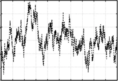
variational parameters at observation times, as shown in Figure 1. 247
Figure 1: An example of the local polynomial approximation, on a univariate system. The vertical dashed lines represent the times the observations occur and each polynomial is defined locally between two observation times. The filled diamond and circles indicate closed sets, while the clear diamonds define open sets. Note that only the first polynomial is defined in a closed set from both sides, to avoid overlapping.
The expression for the (approximate)Lagrangian for thej’th sub-interval thus becomes: 248 ˜ Lj = ˜Fj(q(Xt),θ,Σ)− Z t∈Tj λ⊤t( ˙mt+ ˜Ajtmt−˜bjt) + tr{Ψt( ˙St+ ˜AjtSt+StA˜jt⊤−Σ)} dt , (13)
whereTj⊂T, orT ={T1∪ · · · ∪Tj∪ · · · ∪TJ}, withJ ≥1, being the total number of disjoint sub-sets. 249
The expressions for the polynomial approximations, Eq. (12), can be presented more compactly using 250
matrix notation. This simplified presentation is used from this point forward: 251
˜
Ajt=Aj×pj(t), ˜
bjt=bj×pj(t). (14)
Schematically these matrix - vector products can be seen as: 252 ˜ Ajt reshape to ← Aj1(t) Aj2(t) .. . AjD2(t) = Aj1,0 Aj1,1 · · · Aj1,M Aj2,0 Aj2,1 · · · Aj2,M .. . ... . .. ... AjD2,0 A j D2,1 · · · A j D2,M | {z } Aj × 1 t .. . tM | {z } pj(t) .
Here Ajr,i represents ther’th (scalar) component of theAji coefficient in thej’th sub-interval. Effectively, 253
we have reshaped the Aji weights in column vectors and packed them all together in one matrix of size 254
D2×(M + 1). For the ˜bjt a similar procedure is followed, which is simpler because the b j
i coefficients are
255
already vectors, so there is no need to reshape them. Hence we have: 256 ˜ bjt ← bj1(t) bj2(t) .. . bjD(t) = bj1,0 bj1,1 · · · bj1,M bj2,0 bj2,1 · · · bj2,M .. . ... . .. ... bjD,0 bjD,1 · · · bjD,M | {z } bj × 1 t .. . tM | {z } pj(t) ,
wherebjr,irepresents ther’th component of the bji coefficient. 257
Eq. (14) shows that the vectors pj(t) can be precomputed off-line for all predefined discrete time do-258
mains, reducing the computational complexity of estimating the coefficients of the polynomials. pj(t) is 259
precomputed and stored column-wise in a matrix, as shown on Table 1. Thus the reconstruction of the ap-260
proximate variational parameters ˜Ajt and ˜b j
t, for their whole time domain, can be done by a simple matrix
261
- matrix multiplication (e.g. ˜Ajt =Aj×Πj(t)).
262 1 1 1 · · · 1 tk+δt tk+2δt tk+3δt · · · tk+1 t2 k+δt t2k+2δt t2k+3δt · · · t2k+1 .. . ... ... . .. ... tMk+δt tMk+2δt tMk+3δt · · · tMk+1
Table 1: Example ofΠj(t) matrix, defined onTj= (t
k, tk+1].
The number of coefficients for both variational parameters ˜Atand ˜btis:
263
Ltotal= (D+ 1)×D×(M + 1)×J , (15)
variables, whereD is the system dimension,M is the order of the polynomials andJ is the total number 264
of disjoint sub-intervals (i.e. the number of observation times increased by one). Usually, it is anticipated 265
thatLtotal≪Ntotal, thus making the optimisation problem smaller.
266
The original VGPA algorithm, uses a scaled conjugate gradient (SCG) algorithm (see Nabney [45]), to 267
minimize Eq.(10) with respect to the variational parametersAt and bt. The same procedure is used here
268
computing the gradients of the approximate Lagrangian Eq.(13), with respect to the coefficients Aj and
269
bj, of the re-parametrized variational parameters, for each sub-interval. To further improve computational 270
efficiency and stability a modified Gram-Schmidt orthogonalisation is applied (Golub and van Loan [23]) 271
to the rows of the pre-computedΠj(t) matrices, as shown in Table 1, on each sub-interval separately. In
272
practice this orthogonalisation dramatically reduces the number of iterations required for the algorithm to 273
reach convergence. 274
4. Numerical simulations on artificial data 275
This section explores the convergence properties of the new Local Polynomial (hereafter LP) approxima-276
tion algorithm comparing to the original VGPA framework. The new LP approach is validated on one linear 277
and two non-linear dynamical systems. The experimental set up will be shown first, followed by results for 278
the uni- and multi-variate systems. 279
4.1. Choice of systems & experimental design
280
The first system considered is the linear one dimensional Ornstein-Uhlenbeck process (OU). Originating 281
from the physics literature it was proposed as a model for the velocity of a particle undergoing Brownian 282
motion (Uhlenbeck and Ornstein [58]). Here it is understood as a continuous Markov process with dynamics 283
that can be represented by the following SDE: 284
dXt=−θXtdt+ Σ1/2dWt, (16)
whereθ >0 is the drift parameter, Σ∈ ℜ is the diffusion coefficient2 andW
t∈ ℜ is the univariate Wiener
285
process. In fact this system is one of very few on which exact inference can be performed. The prior process 286
is Gaussian (linear), and given that the initial state is fixed (X0 = x0), the (non-stationary) covariance
287
function for the posterior process is given by: 288
Cov(Xt, Xs) = Σ
2θ(exp{−θ|t−s|} −exp{−θ(t+s)}), (17) which can then be used in a Gaussian process regression smoother to compute the exact posterior (Rasmussen 289
and Williams [51]). 290
2To keep the notation consistent we use Σ instead ofσ2, and we represent the scalars with normal fonts while vectors and
0 2 4 6 8 10 12 14 16 18 20 −1.5 −1 −0.5 0 0.5 1 1.5 t X(t)
Figure 2: An example of the Ornstein-Uhlenbeck diffusion process that will be used later in the simulations.
Secondly, the non-linear double well model (DW), which is a stochastically forced scalar differential 291
equation with three equilibrium values atXt= 0 andXt=±θ (Miller et al. [44]) is considered. As shown
292
in Fig. 3(a) the position of a particle at 0 is unstable, while stable equilibria are found at±θin the absence 293
of noise. Mathematically, the potential is given by U(x) = −2x2+x4. Notice that the drift function in
294
Eq. (18), is simply the derivative: −dUdx(x) = 4x(1−x2), for θ = 1. However, within our setting random
295
forces occur and occasionally drive the particle from one basin to the other (see Fig. 3(b)). This effect is 296
known as “transition” between the two stable states. The SDE that describes the dynamics of this system 297
is the following: 298
dXt= 4Xt(θ−Xt2)dt+ Σ1/2dWt, (18) where θ > 0, is the drift parameter which determines the stable points. Although a simple system, the 299
double well has served as a benchmark in a number of references such as [19, 5]. 300 −2 −1 0 1 2 −1 0 1 2 3 4 5 6 7 8 x U(x)
(a) Double well potential
0 2 4 6 8 10 12 14 16 18 20 −2 −1.5 −1 −0.5 0 0.5 1 1.5 t X(t)
(b) Double well simulation
Figure 3: (a) The double well potential. The circles indicate the stable points (in this example±1), in the absence of stochastic forcing, while the triangle denotes the unstable point. (b) An example of a DW sample path including a transition. This sample path will be used as the history in the experimental simulations.
The final system is a stochastic version of the three dimensional chaotic Lorenz ’63 (L3D), driven by the 301 following SDE: 302 dXt= σ(yt−xt) ρxt−yt−xtzt xtyt−βzt dt+Σ1/2 dW t, (19)
where Xt = [xt yt zt]⊤ ∈ ℜ3 is the state vector representing all three dimensions, θ = [σ ρ β]⊤ ∈ ℜ3, is
303
the drift parameter vector, Σ ∈ ℜ3×3 is a (diagonal) covariance matrix and W
t ∈ ℜ3 is an uncorrelated
304
multivariate Wiener process. The deterministic version of this model (i.e. without the noisy part of Eq. (19)) 305
was first introduced by Lorenz [40] as a low dimensional analogue for large scale thermal convection in the 306
atmosphere. This multi-dimensional non-linear system produces chaotic behaviour when its drift parameters 307
σ,ρandβ lie within a specific range of values and is used in a large body of literature (see Evensen and van 308
Leeuwen [18], Miller et al. [44] and Hansen and Penland [25]). The choice of the drift values, in this work, 309
are those which produce chaotic behaviour (as shown in Table 2) and are the most commonly used values. 310 0 2 4 6 8 10 12 14 16 18 20 −20 0 20 t X(t) 0 2 4 6 8 10 12 14 16 18 20 −30 0 30 t Y(t) 0 2 4 6 8 10 12 14 16 18 20 0 50 t Z(t)
(a) Lorenz 3D simulation
−205 −15 −10 −5 0 5 10 15 20 10 15 20 25 30 35 40 45 X(t) Z(t) (b) Lorenz 3D in X-Z plane
Figure 4: (a) A typical realisation of the stochastic Lorenz ’63 system as time series in each dimension. (b) The same data but in X-Z plane where the effect of the random fluctuations is more clear.
Following a similar strategy to Apte et al. [3], the time discretisation is applied only in the posterior 311
approximation; the inference problem is derived in an infinite dimensional framework (continuous time 312
sample paths), as shown in Section 2.2. The Euler-Maruyama representation of the prior process (3), leads 313
to the following discrete time analogue 314
xk+1=xk+f(t,xk;θ)δt+
√
Σδtξk, (20)
whereξk ∼ N(0,I) and the positiveinfinitesimal dt in Eq.(3), has now been replaced by a positive finite
System t0 tf δt θ Σ Nobs R
OU 0 20 0.01 2 1 2 0.04
DW 0 20 0.01 1 0.8 2 0.04
L3D 0 20 0.01 [10,28,2.6667] 6 10 2
Table 2: Experimental setup that generated the data (trajectories and observations). Initial times (t0) and final times (tf)
define a fixed time window of inference, whilstδtis the time discretisation step. θ are the parameters related to the drift
function, whileΣandRrepresent the noise (co)variances of the stochastic process and the discrete observations accordingly.
In the multivariate system these covariance matrices are diagonal. Nobsrepresents the number of available i.i.d. observations
per time unit (i.e. observation density), which without loss of generality is measured at equidistant time instants.
number δt. In addition, this expression can be used to provide approximate sample paths (in terms of 316
discretising a stochastic differential equation) from the prior process (Higham [26], Kloeden and Platen 317
[35]). Under this first order approximation we impose a suitably small discretisation stepδtto achieve good 318
accuracy. 319
In the numerical experiments a fixed inference window of twenty time units (i.e. T = [0,20]) was 320
considered for all systems and the time discretisation was set toδt= 0.01 for numerical stability. For the 321
L3D the deterministic equations were integrated forwards in time for Tburn = 5000 units, in order to get
322
the initial state vectorX0on the attractor and then generated the stochastic sample path (Figures 4(a) and
323
4(b)). Table 2 summarizes thetrue parameter values, that generated the sample paths for the simulations 324
that follow. Note that 20 time units within these systems corresponds to a rather long assimilation window 325
compared with operational systems. 326
4.2. State estimation results
327
The presentation of the experimental simulations begins with results for the OU process. Figure 5 shows 328
the results from the LP approximation of the VGPA algorithm, of polynomial orderM = 5. For this example 329
the measurement density of 2 observations per time unit (hence 40 in the whole time domainT = [0,20]), 330
withM = 5 andJ = 41, produces a set ofLtotal= 492 coefficients to be inferred, compared toNtotal= 4000
331
in the original VGPA framework. This is roughly 12.3% of the size of the original VGPA optimisation 332
problem. For this system, as mentioned earlier, one can use the induced non-stationary covariance kernel 333
function Eq.(17) and compute the exact posterior process. Comparing the results obtained from the LP 334
approximation with the results from a GP regression smoother with the OU kernel the match is excellent, as 335
expected for a linear system, where the approximation is theoretically exact (in the limiting case asδt→0). 336
To provide a robust demonstration of the consistency of the results of the LP approximation, with 337
respect to the original discretized VGPA, fifty different realisations of the observation noise, from a single 338
trajectory, were used. The order of the polynomials was increased to explore convergence of the LP to the 339
0 2 4 6 8 10 12 14 16 18 20 −1.5 −1 −0.5 0 0.5 1 1.5 2 t m(t) ± (2 × std(t))
Figure 5: The marginal values of the means (solid blue line) and variances (shaded grey area) obtained by the LP approximation of 5’th order on a single realisation of the OU system. The results from the GP regression, on the same observation set, are visually indistinguishable and are omitted. The circles indicate noisy observations.
original VGPA. Summary statistics from these experiments, on the OU system, concerning the convergence 340
of the free energy obtained from the LP approximation algorithm compared with the one from the original 341
VGPA, are shown in Figure 6(a). Here the median is plotted along with the 25’th and 75’th percentiles in 342
box-plots, while the extended vertical dashed lines indicate the 5’th and 95’th percentiles, from these 50 343
realisations, when the system has converged to its free energy minimum. For this example, with only second 344
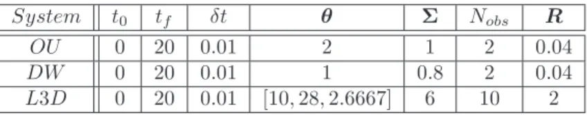
order polynomials (i.e. M = 2), the LP algorithm reaches the same free energy values as the original VGPA. 345 1 2 3 4 5 6 7 8 9 10 11 12 13 14 15 16 17 18 19 20 24 26 28 30 32 34 36 38 40 F(M) M
(a) Variational free energy
1 2 3 4 5 6 7 8 9 10 11 12 13 14 15 16 17 18 19 20 30 40 50 60 70 80 90 100 Nit(M) M (b) Number of SCG iterations
Figure 6: (a) The median and the 25’th to 75’th percentiles as box-plots of the variational free energy, from fifty realisations of the observation noise, as a function of the increasing order of polynomials M, keeping the drift and diffusion parameters fixed to their true values. Extended vertical dashed lines indicate the 5’th and 95’th percentiles. The horizontal dashed (blue) line represents the 50’th percentile of the free energy obtained from the original VGPA on the same 50 realisations and the shaded area encloses the 25’th to 75’th percentiles. (b) The summaries from the same experiment concerning the number of iterations both algorithms needed to converge to optimality. Again, the horizontal lines (and shaded area) represent results obtained for the original VGPA, while boxplot results from the LP approximation, as in (a).
Figure 7(a) compares the results obtained from the LP approximation with 5’th order polynomials, on 346
a single realisation of the DW system, to the outcomes of a Hybrid Monte Carlo (HMC) sample from the 347
posterior process, using the true values for the drift and diffusion parameters. The HMC algorithm [13], 348
combines Hamiltonian molecular dynamics with the Metropolis-Hastings accept/reject criterion to propose 349
a new configuration (or a new sample path) of the posterior process (Eq. 4). The algorithm begins with 350
an initial (discrete time) sample pathXj =
{xjk}Nk=0, where j >0 is the step in the iterative process and 351
proposes a new sample pathXj+1 =
{xjk+1}Nk=0. This is done by simulating, forwards in time, a fictitious 352
time deterministic system: 353 dxjk dτ =pk and dpk dτ =− ∂H(xjk, pk) ∂xjk , (21)
wherepk∼ N(0,1) are the fictitious momentum variables assigned to each state variable xk, resulting in a
354
finite size random vectorp={pk}Nk=0. These deterministic equations are discretised with a time step δτ
355
and solved with aleapfrog integration scheme. The Hamiltonian of the systemH(X,p) is: 356
H(X,p) =Epot+Ekin, (22)
whereEpot=−lnp(Xt0:tf|Y1:K) is the potential energy associated with the dynamics of the system (SDE) 357
as well as the observations Eq.(4) andEkin= 12pp⊤ is the kinetic energy.
358
The HMC solution is assumed to provide a reference solution to the smoothing problem. The setting 359
for the DW example is 25,000 iterations of which the first 5,000 are considered as a burn-in period and 360
discarded. Each HMC iteration generates 80 posterior sample paths (or configurations) of the system with 361
artificial time δτ = 0.01, of which only the last one is considered as candidate state. In total 2,000,000 362
sample paths are generated from which only 20,000 are sampled uniformly to compute the marginal mean 363
and variance as shown in Figure 7(a). The convergence results of this simulation are shown in Figure 7(b). 364
Even though there exist recently proposed MC sampling algorithms, such as thegeneralised HMC as suggest 365
by Alexander et al. [1] to speed up the convergence of the Markov chain, here a rather classical hybrid Monte 366
Carlo, as was first introduced by Duane et al. [13] is used. 367
Although the variance of the LP approximation is slightly underestimated, the mean path matches the 368
HMC results and the time of the transition between the two wells is tracked accurately. The variational 369
approximation as shown in Section 2.2 is likely to underestimate the variance of the approximating process, 370
as is often the case when the expectation in the KL divergence is taken with respect to the approximating 371
distribution3 in Eq.(5). Empirically we have found this to have a relatively minor impact as long as the
372
system is well observed, which keeps the posterior process close to Gaussian. Where the true posterior process 373
3That isKL[q
tkpt] instead of computingKL[ptkqt], whereptis the true posterior whileqtis the approximate one.
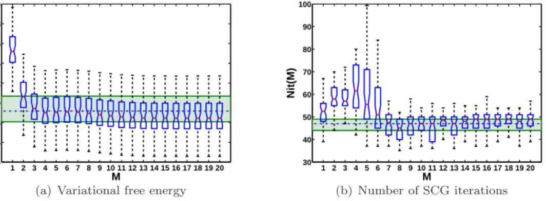
is strongly non-Gaussian, and in particular where it is multi-modal there is more significant underestimation, 374 as might be expected. 375 0 2 4 6 8 10 12 14 16 18 20 −2 −1.5 −1 −0.5 0 0.5 1 1.5 2 t m(t) ± (2 × std(t)) (a) HMC vs LP 100 101 102 103 104 −2000 −1000 0 1000 2000 3000 n (samples) Epot
(b) Potential energy trace
Figure 7:(a) Comparison of the approximate marginal mean and variance (of a single DW realisation), between the “correct” HMC posterior estimates (solid green lines and light shaded area) and the LP approximation, of 5’th order, (dashed blue lines and dark shaded area). The circles indicate noisy observations. (b) Trace of the potential energy (-x- axis is in log-space), of the Hamiltonian, in the HMC posterior sampling. The vertical dashed line, indicates the end of the burn in period and the beginning of the posterior sampling.
Figures 8(a) and 8(b), present results comparable to Figures6(a) and 6(b), but for the DW system. 376
Again 50 different realisations of the observation noise, from a single trajectory, were generated and both 377
LP approximation and VGPA algorithms were applied, given the true parameter values for the drift and 378
diffusion coefficients. The summaries from these runs show the consistency of the LP approximation, when 379
applied to non-linear systems. The algorithm exhibits stability and slightly outperforms the original VGPA 380
framework, in terms of minimizing the free energy, although this has a very minor impact in terms of solving 381
the ODEs (Eq. 7, 8) to produce the marginal means and variances as shown in Figure 7(a). 382 1 2 3 4 5 6 7 8 9 10 11 12 13 14 15 16 17 18 19 20 10 15 20 25 30 F(M) M
(a) Variational free energy
1 2 3 4 5 6 7 8 9 10 11 12 13 14 15 16 17 18 19 20 60 70 80 90 100 110 120 130 Nit(M) M (b) Number of SCG iterations
Figure 8:(a) Similar to Fig.6(a), but from fifty different realizations of the observation noise of the DW system. (b) Again, similar to Fig.6(b), but for the DW system.
To provide a more complete assessment of how this new LP approximation approach to the VGPA 383
algorithm scales with higher dimensions the same experiments were repeated on a multivariate system, 384
namely the Lorenz ’63 (L3D). Figures 9(a) and 9(b), show the approximated mean paths obtained with a 385
3’rd order LP algorithm, against the posterior mean paths computed using HMC, in XY and XZ planes 386
respectively, from a single realisation of the stochastic L3D shown in Figure 4(a). The observation density 387
for this example was relatively high (Nobs= 10, per time unit), hence it was possible to set the order of the
388
polynomials toM = 3. In this example, unlike the previous case of the DW, the LP approximation slightly 389
overestimates the marginal variance (Figure 10(b)) compared with the estimates obtained by using HMC. 390
However, the same effect is observed when applying also the original VGPA framework, hence this is not an 391
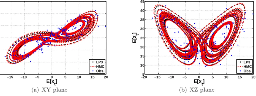
artefact of the polynomial approximation but rather of the variational framework. 392 −20 −15 −10 −5 0 5 10 15 20 −30 −20 −10 0 10 20 30 E[x t] E[y t ] LP3 HMC Obs. (a) XY plane −205 −15 −10 −5 0 5 10 15 20 10 15 20 25 30 35 40 45 E[x t] E[z t ] LP3 HMC Obs. (b) XZ plane
Figure 9: The marginal means, obtained from the LP approximation and the HMC sampling in XY (a) and XZ (b) planes respectively, on a single realisation of the L3D (see Fig. 4(b)). In both plots, the dots (black) are the results from the LP approximation (of 3’rd order), while the squares (red) are results from HMC. Crosses (blue) indicate the noisy observations. TheE[·] notation in the figures axis representsexpected value.
The tuning of the HMC sampling scheme was similar to the one used to obtain the posterior estimates 393
for the DW system, only in this case a smaller artificial time step was necessary to correctly sample the 394
posterior process. In total 25,000 iterations of the HMC algorithm were used, with the first 5,000 considered 395
as burn-in. Each HMC iteration produced 50 new configurations of the system (posterior sample paths), 396
where only the last one was proposed as a new configuration. The artificial time step was δτ = 0.004. 397
Sampling from high dimensional distributions, with the HMC, is not a trivial task. Sampling continuous 398
time sample paths, which when discretised result in a large number of random variables that need to be 399
jointly sampled at each iteration is challenging. For the L3D system considered here, we had to sample 400
Nrv= 6003, random variables at each iteration. The trace of the potential energy of the Hamiltonian (for
401
the L3D example), is presented in Fig. 10(a). Considerable effort was expended to ensure that the HMC 402
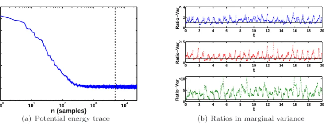
sampler converged and gave a sufficiently uncorrelated set of samples. 403
100 101 102 103 104 0 1000 2000 3000 4000 5000 6000 7000 8000 n (samples) Epot
(a) Potential energy trace
0 2 4 6 8 10 12 14 16 18 20 0 2 4 t Ratio−Var x 0 2 4 6 8 10 12 14 16 18 20 0 5 t Ratio−Var y 0 2 4 6 8 10 12 14 16 18 20 0 5 10 t Ratio−Var z
(b) Ratios in marginal variance
Figure 10: (a) Trace of the potential energy of the Hamiltonian in the HMC posterior sampling of the L3D example. The vertical dashed line, indicates the end of the burn in period and the beginning of the posterior sampling. Notice also the logarithmic scale on the horizontal axis. (b) The ratios, in each dimension of the L3D, between the LP approximate variance over the one obtained by the HMC sampling (i.e. V arLP
V arHMC). The overestimation from the LP approximation is apparent in all three dimensions.
The performance of the new polynomial framework seems to scale well for this multivariate system. As 404
shown in Figures 11(a) and 11(b), when comparing the minimisation of the free energy and the number of 405
iterations to reach convergence, the LP approximation is very stable and fully converges to the original VGPA 406
with onlyM = 2 order of polynomial. The experiments were extended up toM = 20, and showed similar 407
outcomes although with higher computational cost and are omitted from the plots. The observation density 408
considered (i.e. Nobs= 10) implies thatM = 9 is the limit where both algorithms LP and VGPA optimise
409
the same number of parameters. For values ofM >9, the LP becomes more demanding in computational 410
resources. However, when tested with M = 3, we obtain Ltotal = 9,648 whilst Ntotal = 24,000 hence
411
achieving a 59.8% reduction in the number of variables to be optimised. 412 1 2 3 4 5 6 7 8 9 10 1460 1480 1500 1520 1540 1560 1580 1600 1620 1640 F(M) M
(a) Variational free energy
1 2 3 4 5 6 7 8 9 10 250 300 350 400 450 500 Nit(M) M (b) Number of SCG iterations
Figure 11: (a) Box-plots of the free energy attained from 50 realisations of the observation noise (on a single L3D sample path) as a function of the order of polynomialsM. The horizontal dashed line (and the solid ones above and below) represent the 25, 50 and 75 percentiles from the VGPA free energy on the same data sets. (b) Presents a similar plot but for the number of iterations in the SCG optimisation routine at which convergence was achieved. In both plots the extreme values (outliers) have been removed for better presentation.
The reduction in the memory requirements of the algorithm does not produce a similar reduction in 413
computational time. Figures 6(b), 8(b) and 11(b) compare the number of iterations of the LP algorithm 414
to reach convergence with the number of iterations from the VGPA. These results are summaries from 50 415
different realizations (of the observation noise on a single trajectory) of the OU, DW and L3D systems 416
respectively, and show that the original VGPA algorithm, while optimising a larger number of parameters, 417
still converges in slightly fewer iterations. 418
5. Parameter estimation in stochastic systems 419
The original VGPA algorithm can be used to estimate unknown model parameters (Archambeau et al. 420
[5]). The new LP algorithm is also able to estimate the (hyper-) parameters of the aforementioned dynamical 421
systems. In this work the focus is on estimating the drift parametersθand diffusion coefficientsΣ, although 422
estimation of the prior distribution over the initial state (i.e. N(µ0, τ0)) and the noise related to the
423
observationsRcan also be included. 424
The classical approach to parameter estimation, from incomplete data, is the Expectation-Maximization 425
(EM) algorithm, that was first introduced by Dempster et al. [10] and later extended to partially observed 426
diffusions by Dembo and Zeitouni [9]. However, even though the EM algorithm is well studied with a broad 427
range of applications it cannot be applied successfully in the current variational framework, because the 428
approximate posterior distributionqt, induced by Eq. (6), is restricted to have the same diffusion coefficient
429
Σ. Therefore, although an EM approach can be used to estimate the drift parametersθ, the system noiseΣ 430
would have to be held constant during the Maximization step. As a result a different approach for estimating 431
the parameters is adopted. 432
Based on the fact that the variational free energy, Eq. (5), provides an upper bound to the negative 433
log-marginal likelihood (details are in Vrettas et al. [60]): 434
−lnp(Y|θ,Σ) = F(q(X|Σ),θ,Σ)−KL[q(X|Σ)kp(X|Y,θ,Σ)]
≤ F(q(X|Σ),θ,Σ), (23)
whereKL[qkp]≥0, is the Kullback-Leibler divergence between the approximate and correct posteriors and 435
the time dependence has been omitted, two approaches are considered. Initially a discrete approximation to 436
the posterior is constructed, based on a fixed set of possible parameter values. Subsequently gradient based 437
methods are developed to find the approximate “maximum a posteriori” (MAP) values of the parameters. 438
5.1. Discrete approximations to the posterior distribution
439
As seen from Equation (23), the negativefree energy can be substituted for the log marginal likelihood 440
and by choosing suitable prior distributions p0(θ) andp0(Σ), with θ and Σ treated as random variables.
441
To illustrate this approach an example, for the drift parameterθis given. 442
Keeping the diffusion noiseΣfixed to its true value, initially select a set of pointsDθ={θi}ni=1θ at which
443
to approximate the posterior distribution. Run the variational approximation to convergence with these 444
selected values. This yields a corresponding set of free energy valuesDF={F(q(X),θi,Σ)}ni=1θ that can be
445
used to evaluate exp{−F(q(X),θi,Σ)} instead of the true likelihoodp(Y|θ,Σ). Thus
446 p(θ|Y,Σ)∝ exp{−F(q(X|Σ),θi,Σ)} ×p0(θi) nθ i=1 , (24)
wherenθ∈Nis the number of discrete points. Similar discrete approximations, to the posterior distribution,
447
can be computed for the system noiseΣ. In the above procedure the parameters that are not approximated 448
are kept fixed (to their true values). In the results that follow Gamma priors are defined for the drift 449
parameters and inverse Gamma for the system noise covariance, i.e. p0(θ) =G(α, β) andp0(Σ) =G−1(a, b).
450
The values of the parameters α, β, a and b, were chosen such that the mean value of the distribution 451
coincides to the true values ofθ and Σ, but with large variance to reflect our “ignorance” about the true 452
values of the parameters. 453
Figure 12(a), compares the profile of the approximate marginal likelihood, of the OU drift parameter, 454
obtained with the original variational framework (VGPA) and the local polynomial (LP), on a typical 455
realisation. For this system we also show the “true” marginal likelihood obtained using a Gaussian process 456
regression smoother (with OU kernel function). The LP framework converges to the original VGPA when 457
4’th order polynomials are employed, which is consistent with the state estimation results in Fig 6(a). The 458
minimum of the profile can be well identified with only 2’nd order polynomials, which suggests that for the 459
drift parameter, in this example, the bound on the true likelihood does not need to be very precise, if a 460
point estimator is sought. 461
Figure 12(b), shows the results from the LP (of 4’th order) discrete approximation to the posterior 462
distribution of the drift parameter θ using a G(4.0,0.5) prior. Here the results are compared with 80,000 463
samples from the posterior (presented as a histogram), obtained from four independent Markov chains 464
(20,000 samples per chain), using HMC sampling. The same prior distribution (continuous green line) is 465
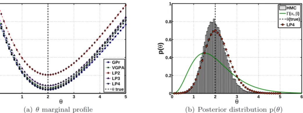
0 1 2 3 4 5 28 30 32 34 36 38 θ F( θ ) GPr VGPA LP2 LP3 LP4 θ true
(a)θmarginal profile
0 1 2 3 4 5 6 0 0.2 0.4 0.6 0.8 1 θ p( θ ) HMC Γ(α, β) θ(true) LP4 (b) Posterior distribution p(θ)
Figure 12:OU system: (a) The profile marginal likelihood of the drift parameterθ, keeping the system noise Σ fixed to its true value, obtained by the GP regression (blue circles) with the OU kernel, which gives the exact likelihood, against the original VGPA algorithm (green squares) and the new LP extension with different order of polynomials. (b) The histogram of the posterior samples obtained with the HMC. The continuous green line shows theG(4.0,0.5) prior of the (hyper)-parameter θ, while the red circles connected with the dot-dashed line represent the discrete approximation to the posterior distribution obtained by the point estimates of the LP algorithm with 4’th order polynomials. Both the HMC posterior sample histogram and the LP approximation have been normalized, such that the area they define sums to unity. In both figures the vertical dashed line represents the true parameter value that generated the data.
used in both cases and in addition the results are presented such that the areas defined by the histogram 466
and the approximate discrete estimates (red circles), sum to one. Although the results, for both algorithms, 467
are slightly biased the LP algorithm provides a better approximation because for a linear system, such as 468
the OU, the variational Gaussian process yields an optimal approximation while the HMC approximation 469
remains subject to finite sample effects. 470 0 1 2 3 4 5 25 30 35 40 45 50 55 60 65 Σ F( Σ ) GPr VGPA LP2 LP3 LP4 LP5 Σ true
(a) Σ marginal profile
0 0.5 1 1.5 2 2.5 3 3.5 4 4.5 5 0 0.5 1 1.5 2 2.5 Σ p( Σ ) HMC Γ−1(a, b) Σ(true) LP5 (b) Posterior distribution p(Σ)
Figure 13: OU system: (a) Plot similar to Fig. 12(a) only for the system noise Σ and keeping the driftθ fixed to its true value. Again, the results of the GP regression represent the exact marginal likelihood. (b) As Fig. 12(b), only the continuous line now is theG−1(3
.0,2.0) prior of the (hyper-) parameter Σ.
Figures 13(a) and 13(b), show similar profile and posterior results, but for the OU system noise coefficient 471
Σ. It is apparent that for this parameter the LP method needs higher order of polynomials to match the 472
results from the original VGPA. All methods locate the minimum of the profile at a smaller value than 473
the true one. Furthermore, both methods seem to deviate from the true likelihood (blue circles), as the 474
value of this parameter becomes more distant from the true value that generated the data. The same bias 475
effect can also be seen in Figure 13(b), where the LP method (5’th order) is compared with the HMC 476
posterior sampling. However, MCMC methods for sampling this parameter can be problematic due to the 477
high dependencies between the system noise Σ and the states of the systemXt, which results in slow rates of
478
convergence (Roberts and Stramer [52], Golightly and Wilkinson [22]). Again the sameG−1(3.0,2.0) prior
479
(continuous green line), was used for both algorithms. 480 0 0.2 0.4 0.6 0.8 1.0 1.2 1.4 1.6 1.8 2.0 0 10 20 30 40 50 60 70 80 θ F( θ ) VGPA LP1 LP2 LP3
(a)θmarginal profile
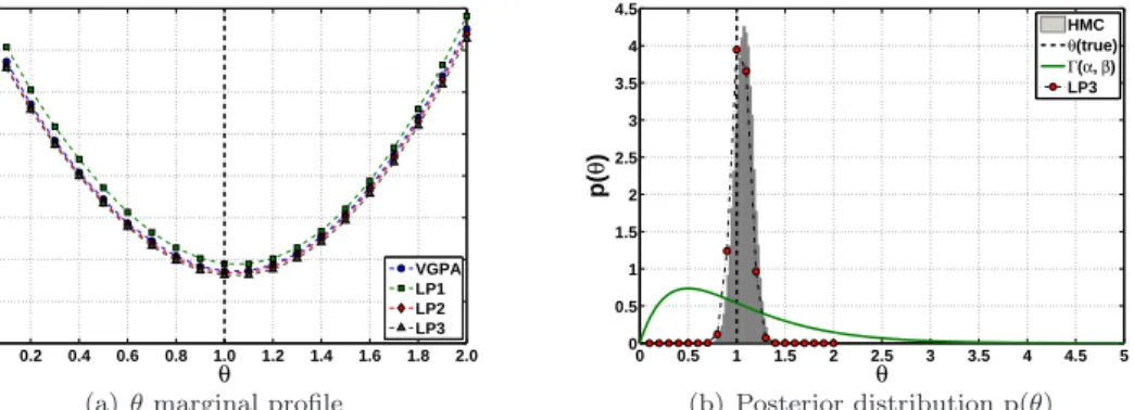
0 0.5 1 1.5 2 2.5 3 3.5 4 4.5 5 0 0.5 1 1.5 2 2.5 3 3.5 4 4.5 θ p( θ ) HMC θ(true) Γ(α, β) LP3 (b) Posterior distribution p(θ)
Figure 14:DW system: (a) The profile approximate marginal likelihood of the drift parameterθ, keeping the system noise Σ fixed to its true value, obtained by original VGPA algorithm (blue circles) and the new LP extension with different order of polynomials. (b) The histogram of the posterior samples obtained using the HMC. The continuous green line shows theG(2.0,0.5) prior of the (hyper-) parameterθ, whilst the red circles connected with the dot-dashed line represent the approximate posterior distribution obtained by the discrete estimates of the LP algorithm with 3’rd order polynomials. Both the HMC posterior sample histogram and the LP point estimates have been normalized, such that the area they define sums to unity.
Likewise, the approximate posterior distributions and profile likelihoods, for a single realisation of the 481
DW system are presented for the driftθ in Figures 14(a) and 14(b) and for the diffusion coefficient Σ in 482
Figs. 15(a) and 15(b). Here there is no method to compute the exact likelihood, hence the only comparison 483
is between the profiles obtained from the VGPA algorithm against those obtained with the LP method. 484
For both parametersθ and Σ, the results are almost identical with 3’rd order polynomials. Both estimates 485
are biased, the drift towards a higher value, while the noise towards a smaller value, but these biases are 486
consistent with those seen in the HMC posterior samples. 487
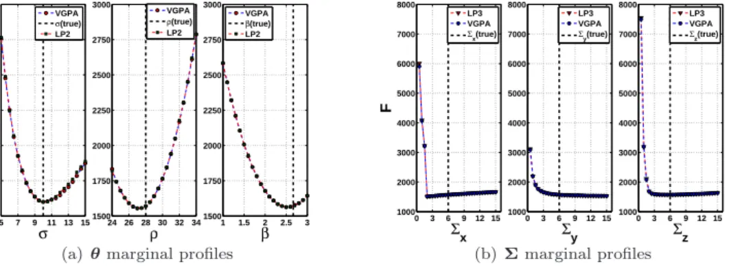
The profiles of the drift parameter vector θ = [σ ρ β]⊤ for the L3D system are shown in Fig. 16(a)
488
where the original VGPA algorithm (red circles) is plotted against the LP approximation, with 2’nd order 489
polynomials (green squares). The results are almost indistinguishable and the minimum values are well 490
estimated for all parameters. Figure 16(b), presents similar profiles but for the diagonal elements of theΣ 491
matrix (i.e. Σx, Σy and Σz). Both the VGPA and the LP (3’rd order) exhibit identical behaviour; unlike